Quantum computing and information extraction for a dynamical quantum system

Abstract

We discuss the simulation of a complex dynamical system, the so-called quantum sawtooth map model, on a quantum computer. We show that a quantum computer can be used to efficiently extract relevant physical information for this model. It is possible to simulate the dynamical localization of classical chaos and extract the localization length of the system with quadratic speed up with respect to any known classical computation. We can also compute with algebraic speed up the diffusion coefficient and the diffusion exponent both in the regimes of Brownian and anomalous diffusion. Finally, we show that it is possible to extract the fidelity of the quantum motion, which measures the stability of the system under perturbations, with exponential speed up.

I Introduction

One of the main applications of computers is the simulation of dynamical models describing the evolution of complex systems. From the viewpoint of quantum computation, quantum mechanical systems play a special role. Indeed, the simulation of quantum many-body problems on a classical computer is a difficult task as the size of the Hilbert space grows exponentially with the number of particles. For instance, if we wish to simulate a chain of $n$ spin-$\frac{1}{2}$ particles, the size of the Hilbert space is $2^{n}$. Namely, the state of this system is determined by $2^{n}$ complex numbers. As observed by Feynman in the 1980’s feynman , the growth in memory requirement is only linear on a quantum computer, which is itself a many-body quantum system. For example, to simulate $n$ spin-$\frac{1}{2}$ particles we only need $n$ qubits. Therefore, a quantum computer operating with only a few tens of qubits could outperform a classical computer. More recently, a few quantum efficient algorithms have been developed for various quantum systems, ranging from some many-body problems lloyd ; fermions to single-particle models of quantum chaos schack ; georgeot ; bcms01 .

Any quantum algorithm has to address the problem of efficiently extracting useful information from the quantum computer wave function. The result of the simulation of a quantum system is the wave function of this system, encoded in the $n$ qubits of the quantum computer. The problem is that, in order to measure all $N=2^{n}$ wave function coefficients by means of standard polarization measurements of the $n$ qubits, one has to repeat the quantum simulation a number of times exponential in the number of qubits. This procedure would spoil any quantum algorithm, even in the case in which such algorithm could compute the wave function with an exponential gain with respect to any classical computation. Nevertheless, there are some important physical questions that can be answered in an efficient way, and we will discuss a few examples in this paper.

We will discuss a quantum algorithm which efficiently simulates the quantum sawtooth map, a physical model with rich and complex dynamics bcms01 . This system is characterized by very different dynamical regimes, ranging from integrability to chaos, and from normal to anomalous diffusion; it also exhibits the phenomenon of dynamical localization of classical chaotic diffusion. We will show that some important physical quantities can be extracted efficiently by means of a quantum computer:

(i) the localization length of the system, which can be extracted with a quadratic speed up with respect to any known classical computation bcms03 ;

(ii) the diffusion coefficient and the diffusion exponent, both in the regimes of normal (Brownian) and anomalous diffusion; in this case we obtain an algebraic speed up;

(iii) the fidelity of quantum motion, which characterizes the stability of the system under perturbations; for this quantity we achieve an exponential speed up.

The paper is organized as follows: the properties of the sawtooth map model are discussed in Sec. II; our quantum algorithm simulating the quantum dynamics of this model in Sec. III; the quantum computation of the localized regime and the extraction of the localization length in Sec. IV; the quantum simulation of the phenomena of normal and anomalous diffusion and the computation of the diffusion coefficient and diffusion exponent in Sec. V; the quantum computation of the fidelity of quantum motion in Sec. VI; our conclusions are summarized in Sec. VII.

II The sawtooth map

The sawtooth map is a prototype model in the studies of classical and quantum-dynamical systems and exhibits a rich variety of interesting physical phenomena, from complete chaos to complete integrability, normal and anomalous diffusion, dynamical localization, and cantori localization. Furthermore, the sawtooth map gives a good approximation to the motion of a particle bouncing inside a stadium billiard (which is a well-known model of classical and quantum chaos).

The sawtooth map belongs to the class of periodically driven dynamical systems, governed by the Hamiltonian

$$H(\theta,I;\tau)=\frac{I^{2}}{2}+V(\theta)\sum_{j=-\infty}^{+\infty}\delta(\tau-jT)\,,$$ (1)

where $(I,\theta)$ are conjugate action-angle variables ($0\leq\theta<2\pi$). This Hamiltonian is the sum of two terms, $H(\theta,I;\tau)=H_{0}(I)+U(\theta;t)$, where $H_{0}(I)=I^{2}\!/2$ is just the kinetic energy of a free rotator (a particle moving on a circle parametrized by the coordinate $\theta$), while

$$U(\theta;t)=V(\theta)\sum_{j}\delta(\tau-jT)$$ (2)

represents a force acting on the particle that is switched on and off instantaneously at time intervals $T$. Therefore, we say that the dynamics described by Hamiltonian (1) is kicked. The corresponding Hamiltonian equations of motion are

$$\left\{\begin{array}[]{l}\displaystyle\dot{I}=-\frac{\partial{H}}{\partial\theta}=-\frac{dV(\theta)}{d\theta}\sum_{j=-\infty}^{+\infty}\delta(\tau-jT)\,,\\[8.61108pt] \displaystyle\dot{\theta}=\frac{\partial{H}}{\partial{I}}=I\,.\end{array}\right.$$ (3)

These equations can be easily integrated and one finds that the evolution from time $lT^{-}$ (prior to the $l$-th kick) to time $(l+1)T^{-}$ (prior to the $(l+1)$-th kick) is described by the map

$$\left\{\begin{array}[]{l}\displaystyle\bar{I}=I+F(\theta)\,,\\[8.61108pt] \displaystyle\bar{\theta}=\theta+T\bar{I}\,,\end{array}\right.$$ (4)

where $F(\theta)=-dV(\theta)/d\theta$ is the force acting on the particle.

In the following, we will consider the special case $V(\theta)=-k(\theta-\pi)^{2}/2$. This map is called the sawtooth map, since the force $F(\theta)=-dV(\theta)/d\theta=k(\theta-\pi)$ has a sawtooth shape, with a discontinuity at $\theta=0$. By rescaling $I\to{J=TI}$, the classical dynamics is seen to depend only on the parameter $K=kT$. Indeed, in terms of the variables $(J,\theta)$ map (4) becomes

$$\left\{\begin{array}[]{l}\displaystyle\bar{J}=J+K(\theta-\pi)\,,\\[8.61108pt] \displaystyle\bar{\theta}=\theta+\bar{J}\,.\end{array}\right.$$ (5)

The sawtooth map exhibits sensitive dependence on initial conditions, which is the distinctive feature of classical chaos: any small error is amplified exponentially in time. In other words, two nearby trajectories separate exponentially, with a rate given by the maximum Lyapunov exponent $\lambda$, defined as

$$\lambda=\lim_{|t|\to\infty}\frac{1}{t}\ln\!\left(\frac{\delta(t)}{\delta(0)}\right),$$ (6)

where the discrete time $t=\tau/T$ measures the number of map iterations and $\delta(t)=\sqrt{[\delta J(t)]^{2}+[\delta\theta(t)]^{2}}$. To compute $\delta J(t)$ and $\delta\theta(t)$, we differentiate map (5), obtaining

$$\left[\begin{array}[]{c}\delta\bar{J}\\ \delta\bar{\theta}\end{array}\right]=M\left[\begin{array}[]{c}\delta J\\ \delta\theta\end{array}\right]=\left[\begin{array}[]{c@{\quad}c}1&K\\ 1&1+K\end{array}\right]\left[\begin{array}[]{c}\delta J\\ \delta\theta\end{array}\right].$$ (7)

The iteration of map (7) gives $\delta J(t)$ and $\delta\theta(t)$ as a function of $\delta J(0)$ and $\delta\theta(0)$ [$\delta J(0)$ and $\delta\theta(0)$ represent a change of the initial conditions]. The stability matrix $M$ has eigenvalues $\mu_{\pm}=\frac{1}{2}(2+K\pm\sqrt{K^{2}+4K})$, which do not depend on the coordinates $J$ and $\theta$ and are complex conjugate for $-4\leq{K}\leq 0$ and real for $K<-4$ and $K>0$. Thus, the classical motion is stable for $-4\leq{K}\leq 0$ and completely chaotic for $K<-4$ and $K>0$. For $K>0$, $\delta(t)\propto(\mu_{+})^{t}$ asymptotycally in $t$, and therefore the maximum Lyapunov exponent is $\lambda=\ln\mu_{+}$. Similarly, we obtain $\lambda=\ln|\mu_{-}|$ for $K<-4$. In the stable region $-4\leq{K}\leq 0$, $\lambda=0$.

The sawtooth map can be studied on the cylinder [$J\in(-\infty,+\infty)$], or on a torus of sinite size ($-{\pi}L\leq J<\pi L$, where $L$ is an integer, to assure that no discontinuities are introduced in the second equation of (5) when $J$ is taken modulus $2{\pi}L$). Although the sawtooth map is a deterministic system, for $K>0$ and $K<-4$ the motion of a trajectory along the momentum direction is in practice indistinguishable from a random walk. Thus, one has normal diffusion in the action (momentum) variable and the evolution of the distribution function $f(J,t)$ is governed by a Fokker–Planck equation:

$$\frac{\partial{f}}{\partial{t}}=\frac{\partial}{\partial{J}}\left(\frac{1}{2}D\frac{\partial{f}}{\partial{J}}\right).$$ (8)

The diffusion coefficient $D$ is defined by

$$D=\lim_{t\to\infty}\frac{\langle(\Delta{J}(t))^{2}\rangle}{t}\,,$$ (9)

where $\Delta{J}\equiv{J}-\langle{J}\rangle$, and $\langle\dots\rangle$ denotes the average over an ensemble of trajectories. If at time $t=0$ we take a phase space distribution with initial momentum $J_{0}$ and random phases $0\leq\theta<2\pi$, then the solution of the Fokker–Planck equation (8) is given by

$$f(J,t)=\frac{1}{\sqrt{2\pi Dt}}\,\exp\!\left[-\frac{(J-J_{0})^{2}}{2Dt}\right].$$ (10)

The width $\sqrt{\langle(\Delta J(t))^{2}\rangle}$ of this Gaussian distribution grows in time, according to

$$\langle(\Delta{J}(t))^{2}\rangle\approx D(K)\,t\,.$$ (11)

For $K>1$, the diffusion coefficient is well approximated by the random phase approximation, in which we assume that there are no correlations between the angles (phases) $\theta$ at different times. Hence, we have

$$D(K)\approx\langle(\Delta{J}_{1})^{2}\rangle=\frac{1}{2\pi}\int_{0}^{2\pi}d\theta\,(\Delta{J}_{1})^{2}=\frac{1}{2\pi}\int_{0}^{2\pi}d\theta\,K^{2}(\theta-\pi)^{2}=\frac{\pi^{2}}{3}\,K^{2}\,,$$ (12)

where $\Delta{J}_{1}=\bar{J}-J$ is the change in action after a single map step. For $0<K<1$ diffusion is slowed, due to the sticking of trajectories close to broken tori (known as cantori), and we have $D(K)\approx 3.3\,K^{5/2}$ (this regime is discussed in percival ). For $-4<K<0$ the motion is stable, the phase space has a complex structure of elliptic islands down to smaller and smaller scales, and one can observe anomalous diffusion, that is, $\langle(\Delta{J})^{2}\rangle\propto{t}^{\alpha}$, with $\alpha\neq 1$ (for instance, $\alpha=0.57$ when $K=-0.1$, see Fig. 4 below). The cases $K=-1,-2,-3$ are integrable.

The quantum version of the sawtooth map is obtained by means of the usual quantization rules, $\theta\to\hat{\theta}$ and $I\to{}\hat{I}=-i\partial/\partial\theta$ (we set $\hbar=1$). The quantum evolution in one map iteration is described by a unitary operator $\hat{U}$, called the Floquet operator, acting on the wave function $\psi$:

$$\bar{\psi}=\hat{U}\,\psi=\exp\left[-i\int_{lT^{-}}^{(l+1)T^{-}}d\tau H(\hat{\theta},\hat{I};\tau)\right]\psi\,,$$ (13)

where $H$ is Hamiltonian (1). Since the potential $V(\theta)$ is switched on only at discrete times $lT$, it is straightforward to obtain

$$\bar{\psi}=e^{-iT\hat{I}^{2}\!/2}\,e^{-iV(\hat{\theta})}\,\psi=e^{-iT\hat{I}^{2}\!/2}\,e^{ik(\hat{\theta}-\pi\hat{\openone})^{2}\!/2}\,\psi\,,$$ (14)

where $\hat{\openone}$ denotes the identity operator. It is important to emphasize that, while the classical sawtooth map depends only on the rescaled parameter $K=kT$, the corresponding quantum evolution (14) depends on $k$ and $T$ separately. The effective Planck constant is given by $\hbar_{\text{eff}}=T$. Indeed, if we consider the operator $\hat{J}=T\hat{I}$ ($\hat{J}$ is the quantization of the classical rescaled action $J$), we have

$$[\hat{\theta},\hat{J}]=T[\hat{\theta},\hat{I}]=iT=i\hbar_{\textbf{eff}}.$$ (15)

The classical limit $\hbar_{\text{eff}}\to 0$ is obtained by taking $k\to\infty$ and $T\to 0$, while keeping $K=kT$ constant.

III Quantum computing of the quantum sawtooth map

In the following, we describe an exponentially efficient quantum algorithm for simulation of the map (14) bcms01 . It is based on the forward/backward quantum Fourier transform between momentum and angle bases. Such an approach is convenient since the operator $\hat{U}$, introduced in Eq. (13), is the product of two operators, $\hat{U}_{k}=e^{ik(\hat{\theta}-\pi\hat{\openone})^{2}\!/2}$ and $\hat{U}_{T}=e^{-iT\hat{I}^{2}\!/2}$, diagonal in the $\theta$ and $I$ representations, respectively. This quantum algorithm requires the following steps for one map iteration:

1. We apply $\hat{U}_{k}$ to the wave function $\psi(\theta)$. In order to decompose the operator $\hat{U}_{k}$ into one- and two-qubit gates, we first of all write $\theta$ in binary notation:

   $$\theta=2\pi\sum_{j=1}^{n}\alpha_{j}2^{-j}\,,$$ (16)

   with $\alpha_{i}\in\{0,1\}$. Here $n$ is the number of qubits, so that the total number of levels in the quantum sawtooth map is $N=2^{n}$. From this expansion, we obtain

   $$(\theta-\pi)^{2}=4\pi^{2}\sum_{j_{1},j_{2}=1}^{n}\left(\frac{\alpha_{j_{1}}}{2^{j_{1}}}-\frac{1}{2n}\right)\left(\frac{\alpha_{j_{2}}}{2^{j_{2}}}-\frac{1}{2n}\right),$$ (17)

   that is

   $$(\hat{\theta}-\pi\hat{\openone})^{2}=4\pi^{2}\sum_{j_{1},j_{2}=1}^{n}\hat{\openone}_{1}\otimes\cdots\otimes\hat{\openone}_{j_{1}-1}\otimes\hat{O}_{j_{1}}\otimes\hat{\openone}_{j_{1}+1}\otimes\cdots\otimes\hat{\openone}_{j_{2}-1}\otimes\hat{O}_{j_{2}}\otimes\hat{\openone}_{j_{2}+1}\otimes\cdots\otimes\hat{\openone}_{j_{n}},$$ (18)

   where $\hat{\openone}_{j}$ is the identity operator for the qubit $j$ and the one-qubit operators $\hat{O}_{j_{1}}$ and $\hat{O}_{j_{2}}$ act on qubits $j_{1}$ and $j_{2}$, respectively. We have

   $$\hat{O}_{j}=\frac{1}{2^{j}}\frac{\hat{\openone}_{j}-(\hat{\sigma}_{z})_{j}}{2}-\frac{1}{2n}\hat{\openone}_{j},$$ (19)

   where $(\hat{\sigma}_{z})_{j}$ denotes the Pauli operator $\hat{\sigma}_{z}$ for the qubit $j$. Note that the operator $\hat{O}_{j}$ is diagonal in the computational basis $\{|0\rangle,|1\rangle\}$. We can insert (18) into the unitary operator $\hat{U}_{k}$, obtaining the decomposition

   $$e^{ik(\hat{\theta}-\pi\hat{\openone})^{2}\!/2}=\prod_{j_{1},j_{2}=1}^{n}\exp\!\left[i2\pi^{2}k\left(\hat{\openone}_{1}\otimes\cdots\otimes\hat{\openone}_{j_{1}-1}\otimes\hat{O}_{j_{1}}\otimes\hat{\openone}_{j_{1}+1}\otimes\cdots\otimes\hat{\openone}_{j_{2}-1}\otimes\hat{O}_{j_{2}}\otimes\hat{\openone}_{j_{2}+1}\otimes\cdots\otimes\hat{\openone}_{j_{n}}\right)\right],$$ (20)

   which is the product of $n^{2}$ two-qubit gates (controlled phase-shift gates), each acting non-trivially only on the qubits $j_{1}$ and $j_{2}$. In the computational basis $\{|\alpha_{j_{1}}\alpha_{j_{2}}\rangle=|00\rangle,|01\rangle,|10\rangle,|11\rangle\}$ each two-qubit gate can be written as $\exp(i2\pi^{2}kD_{j_{1},j_{2}})$, where $D_{j_{1},j_{2}}$ is a diagonal matrix:

   $$D_{j_{1},j_{2}}=\left[\begin{array}[]{cccc}\frac{1}{4n^{2}}&0&0&0\\ 0&-\frac{1}{2n}\big{(}\frac{1}{2^{j_{2}}}-\frac{1}{2n}\big{)}&0&0\\ 0&0&-\frac{1}{2n}\big{(}\frac{1}{2^{j_{1}}}-\frac{1}{2n}\big{)}&0\\ 0&0&0&\big{(}\frac{1}{2^{j_{1}}}-\frac{1}{2n}\big{)}\big{(}\frac{1}{2^{j_{2}}}-\frac{1}{2n}\big{)}\end{array}\right].$$ (21)

   Note that decomposition (20) of $\hat{U}_{k}$ is specific to the sawtooth map.

2. The change from the $\theta$ to the $I$ representation is obtained by means of the quantum Fourier transform, which requires $n$ Hadamard gates and $\frac{1}{2}n(n-1)$ controlled phase-shift gates (see, e.g., nielsenchuang ).

3. In the $I$ representation, the operator $\hat{U}_{T}$ has essentially the same form as the operator $\hat{U}_{k}$ in the $\theta$ representation, and therefore it can be decomposed into $n^{2}$ controlled phase-shift gates, similarly to Eq. (20).

4. We return to the initial $\theta$ representation by application of the inverse quantum Fourier transform.

Thus, overall, this quantum algorithm requires $3n^{2}+n$ gates per map iteration ($3n^{2}-n$ controlled phase-shifts and $2n$ Hadamard gates). This number is to be compared with the $O(n2^{n})$ operations required by a classical computer to simulate one map iteration by means of a fast Fourier transform. Thus, the quantum simulation of the quantum sawtooth map dynamics is exponentially faster than any known classical algorithm. Note that the resources required to the quantum computer to simulate the evolution of the sawtooth map are only logarithmic in the system size $N$. Of course, there remains the problem of extracting useful information from the quantum-computer wave function. This will be discussed in the subsequent sections.

IV Quantum computing of dynamical localization

Dynamical localization is one of the most interesting phenomena that characterize the quantum behavior of classically chaotic systems: quantum interference effects suppress chaotic diffusion in momentum, leading to exponentially localized wave functions. This phenomenon was first found and studied in the quantum kicked-rotator model izrailev and has profound analogies with Anderson localization of electronic transport in disordered materials fishman . Dynamical localization has been observed experimentally in the microwave ionization of Rydberg atoms koch and in experiments with cold atoms raizen .

Dynamical localization can be studied in the sawtooth map model. In this case, map (14) is studied on the cylinder [$I\in(-\infty,+\infty)$], which is cut-off at a finite number $N$ of levels due to the finite quantum (or classical) computer memory. Similarly to other models of quantum chaos, quantum interference in the sawtooth map leads to suppression of classical chaotic diffusion after a break time $t^{\star}$. For $t>t^{\star}$, while the classical distribution goes on diffusing, the quantum distribution reaches a steady state which decays exponentially over the momentum eigenbasis:

$$W_{m}\equiv\big{|}\langle m|\psi\rangle\big{|}^{2}\approx\frac{1}{\ell}\,\exp\!\left[-\frac{2|m-m_{0}|}{\ell}\right],$$ (22)

with $m_{0}$ the initial value of the momentum (the index $m$ singles out the eigenstates of $\hat{I}$, that is, $\hat{I}|m\rangle=m|m\rangle$) footnote . Therefore, for $t>t^{\star}$ only $\sqrt{\langle(\Delta{m})^{2}\rangle}\sim\ell$ levels are populated.

An estimate of $t^{\star}$ and $\ell$ can be obtained by means of the following argument siberia . The localized wave packet has significant projection over about $\ell$ basis states, both in the basis of the momentum eigenstates and in the basis of the eigenstates of the Floquet operator $\hat{U}$ defined by Eq. (13). This operator is unitary and therefore its eigenvalues can be written as $\exp(i\lambda_{i})$, and the so-called quasienenergies $\lambda_{i}$ are in the interval $[0,2\pi[$. Thus, the mean level spacing between “significant” quasienergy eigenstates is $\Delta E\approx 2\pi/\ell$. The Heisenberg principle tells us that the minimum time required to the dynamics to resolve this energy spacing is given by

$$t^{\star}\approx 1/\Delta E\approx\ell.$$ (23)

This is the break time after which the quantum feature of the dynamics reveals. Diffusion up to time $t^{\star}$ involves a number of levels given by

$$\sqrt{\langle(\Delta{m})^{2}\rangle}\approx\sqrt{D_{m}t^{\star}}\approx\ell,$$ (24)

where $D_{m}=D/T^{2}$ is the classical diffusion coefficient, measured in number of levels. The relations (23) and (24) imply

$$t^{\star}\approx\ell\approx D_{m}.$$ (25)

Therefore, the quantum localization length $\ell$ for the average probability distribution is approximately equal to the classical diffusion coefficient. For the sawtooth map,

$$\ell\approx D_{m}\approx(\pi^{2}\!/3)k^{2}\,.$$ (26)

Note that the quantum localization can take place on a finite system only if $\ell$ is smaller than the system size $N$.

In Fig. 1 (taken from bcms03 ), we show that exponential localization can already be clearly seen with $n=6$ qubits. It is important to stress that in a quantum computer the memory capabilities grow exponentially with the number of qubits (the number of levels $N$ is equal to $2^{n}$). Therefore, already with less than $40$ qubits, one could make simulations inaccessible to today’s supercomputers. Fig. 1 shows that the exponentially localized distribution, appearing at $t\approx{}t^{\star}$, is frozen in time, apart from quantum fluctuations, which we partially smooth out by averaging over a few map steps. The freezing of the localized distribution can be seen from comparison of the probability distributions taken immediately after $t^{\star}$ (the full curve in Fig. 1) and at a much larger time $t=300\approx 25t^{\star}$ (the dashed curve in the same figure). Here the localization length is $\ell\approx 12$, and classical diffusion is suppressed after a break time $t^{\star}\approx\ell\approx{}D_{m}$, in agreement with estimates (25)–(26) [the classical diffusion coefficient is $D_{m}\approx(\pi^{2}\!/3)k^{2}\approx 9.9$]. This quantum computation up to times of the order of $\ell$ requires a number $N_{g}\approx 3n^{2}\ell\sim 10^{3}$ of one- or two-qubit quantum gates.

Figure 1: The probability distribution over the momentum basis for the sawtooth map with $n=6$ qubits, $k=\sqrt{3}$, $K=\sqrt{2}$, and initial momentum $m_{0}=0$; the time average is taken in the intervals $10\leq{t}\leq 20$ (full curve) and $290\leq{t}\leq 300$ (dashed curve). The straight line fit, $W_{m}\propto\exp(-2|m|/\ell)$, gives a localization length $\ell\approx 12$. Note that the logarithm is base ten.

In Fig. 2, we show a quantum computation that might be performed already with a three-qubit quantum processor. It is possible to compare two very different regimes, namely the localized and the ergodic regime, by varying only the value of the quantum parameter $k$, while keeping the classical parameter $K$ constant. In both cases the wave function is stationary (apart from quantum fluctuations), as can be seen from the comparison of the wave function patterns at different times. The difference between the two cases is striking. Notice that, in this example, the localization length $\ell<1$ and one can explain the results of this simulation using perturbation theory. Indeed, we have $k\sim 0.35<1$, and therefore we can treat the kick $\hat{U}_{k}$ as a perturbation of the free-evolution operatore $\hat{U}_{T}$. The case shown in Fig. 2 is interesting since it involves only $n=3$ qubits and a few tens on quantum gates. Therefore this quantum computation seems to be accessible or close to the present capabilities of NMR-based NMR1 ; NMR2 and ion-trap ions quantum processors.

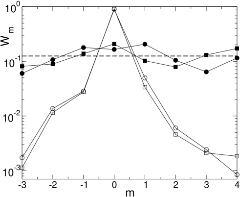
Figure 2: The probability distribution over the momentum basis for the sawtooth map with $n=3$ qubits, $k=K/T=KN/2\pi L$, and initial momentum $m_{0}=0$: ergodic regime at $L=1$ (full symbols) and localized regime at $L=5$ (empty symbols). Circles (squares) represent the wave function after $t=3$ ($t=50$) time steps. The dashed line represents an equally weighted wave function. To smooth the results, we average over ten (one hundred) different values of $K\in[1.4,1.5]$ for the localized (ergodic) case.

We now discuss how to extract the relevant information (the value of the localization length) from a quantum computer simulating the sawtooth-map dynamics. The localization length can be measured by running the algorithm repeatedly up to time $t>t^{\star}$. Each run is followed by a standard projective measurement on the computational (momentum) basis. Since the wave function at time $t$ can be written as

$$|\psi(t)\rangle=\sum_{m}\hat{\psi}(m,t)\,|m\rangle\,,$$ (27)

with $|m\rangle$ momentum eigenstates, such a measurement gives outcome $\bar{m}$ with probability

$$W_{\bar{m}}=\big{|}\langle\bar{m}|\psi(t)\rangle\big{|}^{2}=\big{|}\hat{\psi}(\bar{m},t)\big{|}^{2}\,.$$ (28)

A first series of measurements would allow us to give a rough estimate of the variance $\langle(\Delta{m})^{2}\rangle$ of the distribution $W_{m}$. In turn, $\sqrt{\langle(\Delta{m})^{2}\rangle}$ gives a first estimate of the localization length $\ell$. After this, we can store the results of the measurements in histogram bins of width $\delta{m}\propto\ell\approx\sqrt{\langle(\Delta{m})^{2}\rangle}$. Finally, the localization length is extracted from a fit of the exponential decay of this coarse-grained distribution over the momentum basis. Elementary statistical theory tells us that, in this way, the localization length can be obtained with accuracy $\nu$ after the order of $1/\nu^{2}$ computer runs. It is interesting to note that it is sufficient to perform a coarse-grained measurement to generate a coarse-grained distribution. This means that it will be sufficient to measure the most significant qubits, and ignore those that would give a measurement accuracy below the coarse graining $\delta{m}$. Thus, the number of runs and measurements is independent of $\ell$.

In Fig. 3, we report a simulation of the measurement process. In the left figure we compare the exact probabilities given by the wave function with the result of a complete measurement of all qubits and the result of a coarse-grained measurement. The histograms are built from the same number of computational runs, each followed by a projective measurement. The coarse-grained measurement does not resolve the thinnest structures of the exact wave function. However, it is still possible to extract a good estimate of the localization length $\ell$ from a fit of the exponential decay of the probability distribution $W_{m}$. In the right figure we compare the localization lengths, extracted from the complete and the coarse-grained measurements, as a function of the number $N_{M}$ of projective measurements. Two distinct behaviors are clearly distinguishable: the localization length computed from the complete measurement of all qubits converges slowly to the exact value for the localization length, since a large number of projective measurement is required in order to resolve the exponentially decaying tails. On the contrary, the coarse-grained measurements approaches the exact value after a much smaller number of measurements, even though the fluctuations as a function of the number of measurements are quite large.

It is possible to give a better estimate of the localization length by computing the inverse participation ratio

$$\xi=\frac{1}{\sum_{m}W_{m}^{2}}.$$ (29)

The inverse participation ratio determines the number of basis states significantly populated by the wave function and gives an estimate of the localization length of the system. We have $1\leq\xi\leq N$, with the limiting cases $\xi=1$ and $\xi=N$ corresponding to a wave function delta-peaked ($W_{m}=\delta_{m,m_{0}}$) or uniformly spread ($W_{m}=1/N$). In the localized regime, $\xi\approx\ell/2$. We stress that the inverse participation ratio is almost insensitive to the behavior of exponentially small tails of the wave function. Thus, the estimate $\ell\approx 2\xi$ is quite accurate already with a small number of coarse-grained mesurement (see Fig. 3).

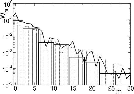
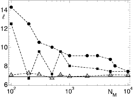
Figure 3: Left: Simulation of a measurement experiment for the quantum sawtooth map at $n=6$, $K=\sqrt{2}$, $T=2\pi L/N$, $L=10$, $t=50$. The thick line is the exact wave function, the thin dashed (thick full) histogram represents the result of $N_{M}$ runs, each followed by a projective measurement of all (all except two) qubits. In both cases $N_{M}=5\times 10^{3}$. Right: The estimated localization length $\ell$ as a function of the number $N_{M}$ of projective measurements. We estimate $\ell$ by fitting the probability decay for the complete (circles) and coarse-grained (squares) measurements. Triangles give $2\xi$, with the inverse partecipation ratio computed from the coarse-grained probability distribution. The straight line is the theoretical result $\ell\sim 6.8$, obtained from Eq. (26).

We now come to the crucial point, of estimating the gain of quantum computation of the localization length with respect to classical computation. First of all, we recall that it is necessary to make about $t^{\star}=O(\ell)$ map iterations to obtain the localized distribution, see Eq. (25). This is true, both for the present quantum algorithm and for classical computation. It is reasonable to use a basis size $N=O(\ell)$ to detect localization (say, $N$ equal to a few times the localization length). In such a situation, a classical computer requires $O(\ell^{2}\log\ell)$ operations to extract the localization length, while a quantum computer would require $O(\ell(\log\ell)^{2})$ elementary gates. Indeed, both classical and quantum computers need to perform $t\approx t^{\star}=O(\ell)=O(N)$ map iterations. Therefore, the quantum computer provides a quadratic speed up in computing the localization length, As we shall see in Sec. VI, the quantum computation can provide an exponential gain (with respect to any known classical computation) in problems that require the simulation of dynamics up to a time $t$ which is independent of the number of qubits. In this case, provided that we can extract the relevant information in a number of measurements polynomial in the number of qubits, one should compare $O(t(\log{N})^{2})$ elementary gates (quantum computation) with $O(tN\log{N})$ elementary gates (classical computation).

V Quantum computing of Brownian and anomalous diffusion

As we have discussed in Sec. II, the classical sawtooth map is characterized by different diffusive behaviors in the chaotic and semi-integrable regimes. Quantum computers could help us to study these different regimes by simulating the map in the deep semiclassical region $\hbar_{\text{eff}}\to 0$. Let us first show that a quantum computer would be useful in computing the Brownian diffusion coefficient $D_{m}$. For this purpose, we can repeat several times the quantum simulation of the sawtooth map up to a given time $t$, ending each run with a standard projective measurement in the momentum basis. This allows us to compute, up to statistical errors, $\langle(\Delta{m})^{2}\rangle$. The diffusion coefficient is then obtained from Eq. (24) as $D_{m}\approx\langle(\Delta{m})^{2}\rangle/t$. Therefore a computation of the diffusion coefficient up to time $t$ significantly involves the order of $\sqrt{D_{m}t}$ momentum eigenstates (other levels are only weakly populated for times smaller than $t$ and can be neglected). Thus, a basis of dimension $N=O(t^{1/2})$ is sufficient for this computation. To estimate the speed up of quantum computation, one should compare $O(t(\log{N})^{2})=O(N^{2}(\log{N})^{2})$ elementary gates (quantum computation) with with $O(tN\log{N})=O(N^{3}\log(N))$ elementary gates (classical computation). This gives an algebraic speed up.

We note that similar computations could be done in the regime of anomalous diffusion, in which $\langle(\Delta J)^{2}\rangle=T^{2}\langle(\Delta m)^{2}\rangle\propto t^{\alpha}$, to evaluate the exponent $\alpha$, a quantity of great physical interest. Such a regime is quite complex in the sawtooth map: Fig. 4 shows, for the classical map, the dependence of the exponent $\alpha$ as a function of $K$. As can be seen from this figure, the map explores subdiffusive ($\alpha<1$) and superdiffusive ($\alpha>1$) regions, up to ballistic diffusion ($\alpha=2$). As required by the principle of quantum to classical correspondence, the quantum sawtooth map follows this behavior in the deep semiclassical regime $\hbar_{\text{eff}}\ll 1$, up to some time scale which diverges when $\hbar_{\text{eff}}\to 0$. It is important to point out that $\hbar_{\text{eff}}$ drops to zero exponentially with the number of qubits ($\hbar_{\text{eff}}\propto 1/N=1/2^{n}$), and therefore the deep semiclassical region can be reached with a small number of qubits. For large $\hbar_{\text{eff}}$, one can also study how diffusion is modified by important quantum phenomena, like quantum tunneling, localization, and quantum resonances.

A quantum computer could help us in obtaining the exponent $\alpha$ of the anomalous diffusion. In this case, since $\langle(\Delta m)^{2}\rangle\propto t^{\alpha}$, a rough estimate of the size of the basis required for the computation up to time $t$ is $N=O(t^{\alpha/2})$. Hence, we must compare $O(t(\log{N})^{2})=O(N^{2/\alpha}(\log{N})^{2})$ elementary gates (quantum computation) with $O(tN\log{N})=O(N^{(\alpha+2)/\alpha}\log(N))$ elementary gates (classical computation). The speed up is again algebraic.

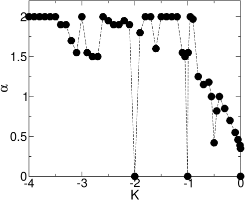
Figure 4: Left: Exponent $\alpha$ of the anomalous diffusion ($\langle(\Delta J)^{2}\rangle\propto t^{\alpha}$) as a function of $K$ for the classical sawtooth map in the semi-integrable regime.

VI Quantum computing of the fidelity of quantum motion

The simulation of quantum dynamics up to a time $t$ which is independent of the number of qubits is useful, for instance, to measure dynamical correlation functions of the form

$$C(t)\equiv\langle\psi|\,\hat{A}^{\dagger}(t)\,\hat{B}(0)\,|\psi\rangle=\langle\psi|\,(\hat{U}^{\dagger})^{t}\,\hat{A}^{\dagger}(0)\,\hat{U}^{t}\,\hat{B}(0)\,|\psi\rangle\,,$$ (30)

where $\hat{U}$ is the time-evolution operator (13) for the sawtooth map. Similarly, we can efficiently compute the fidelity of quantum motion, which is a quantity of central interest in the study of the stability of a system under perturbations (see, e.g., peres ; jalabert ; jacquod ; tomsovic ; PRE ; prosen ; emerson ; zurek and references therein). The fidelity $f(t)$ (also called the Loschmidt echo), measures the accuracy with which a quantum state can be recovered by inverting, at time $t$, the dynamics with a perturbed Hamiltonian. It is defined as

$$f(t)=\langle\psi|\,(\hat{U}^{\dagger}_{\epsilon})^{t}\,\hat{U}^{t}\,|\psi\rangle\,.$$ (31)

Here the wave vector $|\psi\rangle$ evolves forward in time with the Hamiltonian $H$ of Eq. (13) up to time $t$, and then evolves backward in time with a perturbed Hamiltonian $H_{\epsilon}$ ($\hat{U}_{\epsilon}$ is the corresponding time-evolution operator). For instance, we can perturb the parameter $k$ in the sawtooth map as follows: $k\to{}k^{\prime}=k+\epsilon$, with $\epsilon\ll k$. If the evolution operators $\hat{U}$ and $\hat{U}_{\epsilon}$ can be simulated efficiently on a quantum computer, as is the case in most physically interesting situations, then the fidelity of quantum motion can be evaluated with exponential speed up with respect to known classical computations. The same conclusion is valid for the correlation functions (30).

The fidelity can be efficiently evaluated on a quantum computer, with the only requirement of an ancilla qubit, using the scattering circuit drawn in Fig. 5 zoller ; saraceno . This circuit has various important applications in quantum computing, including quantum state tomography and quantum spectroscopy saraceno . The circuit ends up with the measurement of the ancilla qubit, and we have

$$\langle\sigma_{z}\rangle=\mathrm{Re}[\mathrm{Tr}(\hat{W}\rho)],\quad\langle\sigma_{y}\rangle=\mathrm{Im}[\mathrm{Tr}(\hat{W}\rho)],$$ (32)

where $\langle\sigma_{z}\rangle$ and $\langle\sigma_{y}\rangle$ are the expectation values of the Pauli spin operators $\hat{\sigma}_{z}$ and $\hat{\sigma}_{y}$ for the ancilla qubit, and $\hat{W}$ is a unitary operator. These two expectation values can be obtained (up to statistical errors) if one runs several times the scattering circuit. If we set $\rho=|\psi\rangle\langle\psi|$ and $\hat{W}=(\hat{U}_{\epsilon}^{\dagger})^{t}\,\hat{U}^{t}$, it is easy to see that $f(t)=|\mathrm{Tr}(\hat{W}\rho)|^{2}=\langle\sigma_{z}\rangle^{2}+\langle\sigma_{y}\rangle^{2}$. For this reason, provided the quantum algorithm which implements $\hat{U}$ is efficient, as it is the case for the quantum sawtooth map, the fidelity can be efficiently computed by means of the circuit described in Fig. 5. We note that another possible way to efficiently measure the fidelity has been proposed in emerson .

Figure 5: Scattering circuit. The top line denotes the ancilla qubit, the bottom line a set of $n$ qubits, $H$ the Hadamard gate, and $W$ a unitary transformation.

VII Conclusions

In this paper, we have discussed relevant physical examples of efficient information extraction in the quantum computation of a dynamical system. We have shown that a quantum computer with a small number of qubits can efficiently simulate the quantum localization effects, simulate both the Brownian and anomalous diffusion in the deep semiclassical regime, and compute the fidelity of quantum motion. We would like to stress that the simulation of complex dynamical systems is accessible to the first generation of quantum computers with less than 10 qubits. Therefore, we believe that quantum algorithms for dynamical systems deserve further studies, since they are the ideal software for the first quantum processors. Furthermore, we emphasize that the quantum computation of quantities like dynamical localization or fidelity is a demanding testing ground for quantum computers. In the first case, we want to simulate dynamical localization, a purely quantum phenomena which is quite fragile in the presence of noise ott ; song ; in the latter case, fidelity is computed as a result of a sophisticated many-qubit Ramsey-type interference experiment. Therefore the computation of these quantities appears to be a relevant test for quantum processors operating in the presence of decoherence and imperfection effects.