Dynamics and manipulation of entanglement in
coupled harmonic systems with many degrees of freedom

Abstract

We study the entanglement dynamics of a system consisting of a large number of coupled harmonic oscillators in various configurations and for different types of nearest neighbour interactions. For a one-dimensional chain we provide compact analytical solutions and approximations to the dynamical evolution of the entanglement between spatially separated oscillators. Key properties such as the speed of entanglement propagation, the maximum amount of transferred entanglement and the efficiency for the entanglement transfer are computed. For harmonic oscillators coupled by springs, corresponding to a phonon model, we observe a non-monotonic transfer efficiency in the initially prepared amount of entanglement, i.e., an intermediate amount of initial entanglement is transferred with the highest efficiency. In contrast, within the framework of the rotating wave approximation (as appropriate e.g. in quantum optical settings) one finds a monotonic behaviour. We also study geometrical configurations that are analogous to quantum optical devices (such as beamsplitters and interferometers) and observe characteristic differences when initially thermal or squeezed states are entering these devices. We show that these devices may be switched on and off by changing the properties of an individual oscillator. They may therefore be used as building blocks of large fixed and pre-fabricated but programmable structures in which quantum information is manipulated through propagation. We discuss briefly possible experimental realisations of systems of interacting harmonic oscillators in which these effects may be confirmed experimentally.

Submitted to New J. Phys.

I Introduction

Quantum information processing requires as a basic ingredient the ability to transfer quantum information between spatially separated quantum bits, either to implement a joint unitary transformation or, as a special case, to swap quantum information between the qubits. For a transfer over larger distances it is usually imagined that some stationary qubits, for example in the form of trapped ions inside an optical resonator, are coupled to a quantized mode of the electro-magnetic field that propagates between the spatially separated cavities Cirac ZKM 97 ; Duan K 03 ; Feng ZLGX 03 ; Browne PH 03 . Other specific realisations are possible, but the basic principle always relies on the use of some continuous degree of freedom between the qubits and their manipulation by external fields. While this appears to be the most realistic mode of transport over long distances, one may conceive other modes over shorter distances. Instead of using a quantum field one may study the possibilities offered by a discrete set of interacting quantum systems. This might involve spin degrees of freedom Khaneja G 02 ; Bose 02 ; Subrahmanyan 03 ; Christandl DEL 03 ; Osborne L 03 or infinite dimensional systems such as harmonic oscillators Eisert P 03 ; Eisert PBH 03 . In the present paper we explore the dynamics of entanglement in a chain of coupled harmonic oscillators Audenaert EPW 02 ; Brun ; Halliwell . Apart from its obvious relevance to quantum optical systems including photonic crystals, such a model also describes phonons in a crystal and we therefore hope that the results presented here will also have applications in condensed matter systems as well.

This paper is organised as follows. In Section 2 we present the basic physical models and their Hamiltonians. We use analytical tools from the theory of Gaussian states in continuous variable systems where some rapid development has been achieved recently (for a tutorial overview see, e.g., Ref. Eisert P 03 ). We briefly reiterate those results that will be employed in the present investigation. The entanglement properties of a system of harmonic oscillators in the static regime have been studied in some detail Audenaert EPW 02 . Section 3 will then present the basic equations of motion in compact form for two types of interactions, namely (a) harmonic oscillators coupled by springs and, resulting from this, (b) a model which corresponds to a rotating wave approximation as is appropriate in a quantum optical setting. Section 4 employs these equations for the propagation of entanglement along a chain of harmonic oscillators which might be realized by coupled nano-mechanical oscillators Roukes 01 ; Schwab HWR 00 or optical cavities. The time evolution of the entanglement between a pair of oscillators is given analytically in a compact form. Properties such as the speed of propagation, the amount of entanglement and the transfer efficiency are then obtained from these expressions. In Section 5 we present results utilizing the equations from Sections 3 and 4. Firstly, we study a method for the creation of entanglement in such a system that does not require detailed control of the interaction strength between individual oscillators but only the ability for changing the interaction strength globally Eisert PBH 03 . The influence of imperfections such as finite temperatures or randomly varying coupling constants on such a scheme are studied. We also consider the propagation of some initially prepared entangled state along the chain. Surprisingly, for harmonic oscillators coupled by springs we observe a non-monotonic transfer efficiency in the initially prepared amount of entanglement, i.e., an intermediate amount of entanglement is transferred with the highest efficiency. Conversely, in the rotating wave approximation, the transfer efficiency is monotonic. While most of these results assume a position independent and stationary coupling we also show that with carefully chosen position dependent coupling the transfer efficiency in this system may be increased to unity. Finally we study geometrical configurations that are analogous to quantum optical devices such as beamsplitters and interferometers and observe characteristic differences when initially thermal or squeezed states are entering these devices. We show that these devices may be switched on and off by changing the properties of an individual oscillator and may therefore be building blocks of large fixed but programmable structures. In Section 6 we summarize the results of this paper and suggest possible experimental realisations of systems of harmonic oscillators in which these effects may be confirmed.

II Models and Methods

In this section we present the systems under consideration, namely coupled harmonic oscillators, together with the Hamiltonians that describe the various models for their interaction. We will restrict our attention to Hamiltonians that are quadratic in position and momentum operators. This will be crucial for the following analysis as it permits us to draw on the results and techniques from the theory of Gaussian continuous variable entanglement. The most important results from this theory will be reviewed here briefly.

II.1 The physical models

The general setup consists of a chain of $M$ coupled harmonic oscillators, where the coupling is assumed to be such that the corresponding Hamiltonian is at most quadratic in position and momentum. We will number the harmonic oscillators from $1$ to $M$ with periodic boundary conditions such that the $(M+1)$-th oscillator is identified with the $1$-st. The choice of periodic boundary conditions yields exact and compact analytical solutions since we can employ normal coordinates straightforwardly. A similar approach is less successful in the non-periodic boundary case. In addition, we allow for the existence of a distinguished decoupled oscillator with index $0$ which will be a convenient notation for some of the later studies. Arranging the position and momentum operators in the form of a vector

$$R=({\hat{q}}_{0},{\hat{q}}_{1},\ldots,{\hat{q}}_{M},{\hat{p}}_{0},{\hat{p}}_{1},\ldots,{\hat{p}}_{M})$$ (1)

we can then write the general Hamiltonian in the form

$$\hat{H}=\frac{1}{2}R\left[\begin{array}[]{cc}V&0\\ 0&T\end{array}\right]R^{T}=\frac{1}{2}\sum_{ij=1}^{M}{\hat{q}}_{i}V_{ij}{\hat{q}}_{j}+{\hat{p}}_{i}T_{ij}{\hat{p}}_{j},$$ (2)

where $V$ is the potential matrix and $T$ the kinetic matrix. We will consider three basic settings for which we now provide the matrices $T$ and $V$ explicitly. In all these cases we assume that the oscillators in the chain are all identical with a mass $m=1$ and eigenfrequency $\omega=1$.

• (Uncoupled oscillators) If the oscillators are not coupled to each other, then the potential energy of the $k$-th oscillator is simply given by ${\hat{q}}_{k}^{2}/2$ while its kinetic energy is ${\hat{p}}_{k}^{2}/2$. As a consequence, both the potential matrix and the kinetic matrix are diagonal and identical, namely $V=T={\sf 1\rule[0.04303pt]{0.51663pt}{6.54443pt}\rule[0.04303pt]{1.29167pt}{0.51663pt}}_{M+1}$, where ${\sf 1\rule[0.04303pt]{0.51663pt}{6.54443pt}\rule[0.04303pt]{1.29167pt}{0.51663pt}}_{M+1}$ denotes the $M+1$ by $M+1$ identity matrix.

• (Oscillators coupled by springs) If neighbouring oscillators (except for the $0$-th oscillator) are coupled via springs that obey Hooke’s law, the Hamiltonian is given by

  $$\hat{H}_{\rm Spring}=\frac{{\hat{q}}_{0}^{2}+{\hat{p}}_{0}^{2}}{2}+\frac{1}{2}\sum_{k=1}^{M}{\hat{q}}_{k}^{2}+{\hat{p}}_{k}^{2}+c\left(\hat{q}_{k+1}-\hat{q}_{k}\right)^{2},$$ (3)

  where $c$ denotes the coupling strength and we have used periodic boundary conditions i.e., $q_{M+1}=q_{1}$. Keeping in mind that we wish to leave the oscillator with index $0$ uncoupled, the potential matrix becomes

  $$V=\left[\begin{array}[]{ccccccc}1&0&0&0&0&0&0\\ 0&1+2c&-c&0&\cdots&0&-c\\ 0&-c&1+2c&-c&&&0\\ 0&0&-c&1+2c&\ddots&&\vdots\\ \vdots&\vdots&&\ddots&\ddots&-c&0\\ 0&0&&&-c&1+2c&-c\\ 0&-c&0&\cdots&0&-c&1+2c\end{array}\right],$$ (4)

  while the kinetic matrix is given by the identity matrix $T={\sf 1\rule[0.04303pt]{0.51663pt}{6.54443pt}\rule[0.04303pt]{1.29167pt}{0.51663pt}}_{M+1}$.

• (Oscillators in rotating wave approximation) An interaction that provides simpler dynamics is obtained via the rotating wave approximation in quantum optical systems. Indeed, if we define annihilation and creation operators

  $${\hat{a}} = \frac{1}{\sqrt{2}}({\hat{q}}+i{\hat{p}}),\;\;\;\;\;\;{\hat{a}}^{\dagger}=\frac{1}{\sqrt{2}}({\hat{q}}-i{\hat{p}}),$$ (5)

  then we observe that the interaction in case (b) includes terms of the form ${\hat{a}}^{\dagger}_{k}{\hat{a}}^{\dagger}_{k+1}$, i.e., interaction terms for which both harmonic oscillators are being excited simultaneously. Such terms are not energy conserving, and in quantum optics they are usually be neglected in the framework of the rotating wave approximation (RWA). Following this practice amounts to considering the following Hamiltonian

  $$\hat{H}_{\rm RWA} = {\hat{a}}^{\dagger}_{0}{\hat{a}}_{0}+\frac{1}{2}+\sum_{k=1}^{M}(1+c)\Bigl{(}{\hat{a}}^{\dagger}_{k}{\hat{a}}_{k}+\frac{1}{2}\Bigr{)}$$ (6)

  $$- c\left(\hat{a}^{\dagger}_{k+1}\hat{a}_{k}+\hat{a}_{k+1}\hat{a}^{\dagger}_{k}\right).$$

  In terms of position and momentum operators this can be written as

  $$\hat{H}_{\rm RWA} = \frac{{\hat{q}}_{0}^{2}+{\hat{p}}_{0}^{2}}{2}+\frac{1}{2}\sum_{k=1}^{M}{\hat{q}}_{k}^{2}+{\hat{p}}_{k}^{2}$$ (7)

  $$+ \frac{c}{2}\left(\hat{q}_{k+1}-\hat{q}_{k}\right)^{2}+\frac{c}{2}\left(\hat{p}_{k+1}-\hat{p}_{k}\right)^{2},$$

  so that in this case both the potential and the kinetic matrix are given by

  $$T=V=\left[\begin{array}[]{ccccccc}1&0&0&0&0&0&0\\ 0&1+c&-c/2&0&\cdots&0&-c/2\\ 0&-c/2&1+c&-c/2&&&0\\ 0&0&-c/2&1+c&\ddots&&\vdots\\ \vdots&\vdots&&\ddots&\ddots&-c/2&0\\ 0&0&&&-c/2&1+c&-c/2\\ 0&-c/2&0&\cdots&0&-c/2&1+c\end{array}\right].$$ (8)

Note that the matrix $V$ can be conceived as the adjacency matrix of a weighted graph $G(v,e)$ encoding the interaction pattern between the systems in the canonical coordinates corresponding to position. Vertices of the graph correspond to physical systems, i.e., the individual harmonic oscillators, whereas the weight associated with each of the edges quantifies the coupling strength Wolf . The main diagonal corresponds to loops of the weighted graph. This intuition is in immediate analogy to graph states for spin systems with an Ising interaction between the constituents Graphs ; Schlinge ; Rauss and can be useful in the study of more complex geometries. Before we study the dynamical properties of these systems, we provide in the following subsection a brief overview over the main technical tools that we are going to employ.

II.2 Analytical tools

Analysing the entanglement properties of infinite dimensional systems such as harmonic oscillators is generally technically involved unless one restricts attention to specific types of states. Indeed, in recent years a detailed theory of so-called Gaussian entangled states has been developed. As we will employ some of its basic results in the subsequent analysis we are providing a brief review of some useful results. A more detailed tutorial review can be found, e.g., in Ref. Eisert P 03 , and more technical details concerning Gaussian states can be found in Ref. Simon SM 87 .

The relevant variables in the analysis of harmonic oscillators are the canonical operators for position and momentum. Let us assume a system with $n$ harmonic oscillators. As stated above it is convenient to arrange these in the form of a vector

$$R^{T}=({\hat{q}}_{1},\ldots,{\hat{q}}_{n},{\hat{p}}_{1},\ldots,{\hat{p}}_{n})\,.$$

The characteristic feature distinguishing the quantum harmonic oscillator from its classical counterpart is the canonical commutation relation (CCR) between position and momentum. Employing the vector $R$ these can be written in the particularly convenient form $[\hat{R}_{j},\hat{R}_{k}]=i\sigma_{j,k}$ where the real skew-symmetric block diagonal $2n\times 2n$-matrix $\sigma$, the symplectic matrix, given by

$$\sigma=\left[\begin{array}[]{cccccc}0&{{\sf 1\rule[0.04303pt]{0.51663pt}{6.54443pt}\rule[0.04303pt]{1.29167pt}{0.51663pt}}}_{n}\\ -{{\sf 1\rule[0.04303pt]{0.51663pt}{6.54443pt}\rule[0.04303pt]{1.29167pt}{0.51663pt}}}_{n}&0\end{array}\right],$$ (9)

assuming units where $\hbar=1$, and $k=1$, a choice that will be adopted for the rest of this paper. Instead of referring to states, i.e., density operators, one may equivalently refer to functions that are defined on phase space. While there are many equivalent choices for phase space distributions, for the purposes of this work it is most convenient to introduce the (Wigner-) characteristic function. Using the Weyl operator $W_{\xi}=e^{i\xi^{T}\sigma R}$ for $\xi\in{\mathbf{R}}^{2n}$, we define the characteristic function as

$$\chi_{\rho}(\xi)=\mbox{tr}[\rho W_{\xi}].$$ (10)

The state and its characteristic function are related to each other according to a Fourier-Weyl relation,

$$\rho=\frac{1}{(2\pi)^{n}}\int d^{2n}\xi\chi_{\rho}(-\xi)W_{\xi}.$$ (11)

Gaussian states are exactly those states for which the characteristic function $\chi_{\rho}$ is a Gaussian function in phase space Simon SM 87 . That is, if the characteristic function is of the form

$$\chi_{\rho}(\xi)=\chi_{\rho}(0)e^{-\frac{1}{4}(\sigma\xi)^{T}\gamma(\sigma\xi)-d^{T}(\sigma\xi)}.$$ (12)

As is well known, Gaussians are completely specified by their first and second moments, $d$ and $\gamma$ respectively. As the first moments can be always made zero utilizing appropriate local displacements in phase space, they are not relevant in the context of questions related to squeezing and entanglement and will be ignored in the following. The second moments can be collected in the real symmetric $2n\times 2n$ covariance matrix $\gamma$ defined as

$$\gamma_{j,k} = 2\mbox{Re}\,\mbox{tr}\bigl{[}\rho({\hat{R}}_{j}-\langle{\hat{R}}_{j}\rangle_{\rho})({\hat{R}}_{k}-\langle{\hat{R}}_{k}\rangle_{\rho})\bigr{]}\,.$$ (13)

With this convention, the covariance matrix of the $n$-mode vacuum is $\gamma={\sf 1\rule[0.04303pt]{0.51663pt}{6.54443pt}\rule[0.04303pt]{1.29167pt}{0.51663pt}}_{2n}$.

As the covariance matrix encodes the complete information about the entanglement properties of the system, we will use it in order to quantify the amount of entanglement between two groups of oscillators. There is no unique way to quantify entanglement for mixed states, and several different measures grasp entanglement in terms of different operational interpretations. For the purposes of this work we settle for the logarithmic negativity which is comparatively easy to compute and possesses an interpretation as a cost function Audenaert PE 03 ; Lewenstein HSL 98 ; Vidal W 02 ; Eisert P 99 ; Eisert Phd . Given two parties, $A$ and $B$, the logarithmic negativity is defined as

$$N(\rho)=\log_{2}||\rho^{T_{B}}||_{1}$$ (14)

where $\rho^{T_{B}}$ is the state that is obtained from $\rho$ via a partial transposition with respect to system $B$ and $||.||_{1}$ denotes the trace-norm. As we focus attention on Gaussian states which we characterize via the covariance matrix $\gamma$ rather than the density matrix $\rho$, we need to provide a prescription for the evaluation of the logarithmic negativity directly in terms of the covariance matrix. To this end, it is important to note that on the level of covariance matrices the transposition is reflected by time reversal which is a transformation that leaves the positions invariant but reverses all momenta, $\hat{q}\mapsto\hat{q}$, $\hat{p}\mapsto-\hat{p}$. The partial transposition is then the application of this time-reversal transformation to a subsystem, i.e., one party. Let us now consider a system made up of $m+n$ oscillators, where $m$ oscillators are held by party $A$ and $n$ oscillators by party $B$. Applying time reversal to the $n$ oscillators held by party $B$, the covariance matrix will be transformed to a real symmetric matrix $\gamma^{T_{B}}$ given by

$$\gamma^{T_{B}}=P\gamma P,$$ (15)

where

$$P={{\sf 1\rule[0.04303pt]{0.51663pt}{6.54443pt}\rule[0.04303pt]{1.29167pt}{0.51663pt}}}_{m+n}\oplus\left[\begin{array}[]{cc}{\sf 1\rule[0.04303pt]{0.51663pt}{6.54443pt}\rule[0.04303pt]{1.29167pt}{0.51663pt}}_{m}&0\\ 0&-{\sf 1\rule[0.04303pt]{0.51663pt}{6.54443pt}\rule[0.04303pt]{1.29167pt}{0.51663pt}}_{n}\end{array}\right].$$ (16)

The $2n\times 2n$-matrix $\gamma^{T_{B}}$ is the matrix collecting the second moments of the partial transpose $\rho^{T_{B}}$ of $\rho$. The logarithmic negativity is then given by

$$N=-\sum_{j=1}^{m+n}\log_{2}(\min(1,|\gamma_{j}|))\,,$$ (17)

where the $\gamma_{j}$ are the symplectic eigenvalues of $\gamma^{T_{B}}$. For a general covariance matrix, $\gamma_{j}$ arises in the diagonalization of $\gamma$ using symplectic transformations, i.e., transformations $S$ that preserve the CCR so that $S\sigma S^{T}=\sigma$. The resulting diagonal matrix is the Williamson normal form of a covariance matrix whose diagonal elements are the symplectic eigenvalues. It is sometimes useful to know that the symplectic eigenvalues can be obtained directly without explicit diagonalization of the matrix as the positive square roots of the usual eigenvalues of $-\sigma\gamma\sigma\gamma$ Vidal W 02 .

For all Hamiltonians that are quadratic in the canonical position and momentum operators the ground state is an important example of a Gaussian state. For a Hamilton operator of the form

$${\hat{H}}=\frac{1}{2}R^{T}\left[\begin{array}[]{cc}V&0\\ 0&T\end{array}\right]R$$ (18)

we find that the covariance matrix of the ground state is given by

$$\gamma=\sqrt{TV^{-1}}\oplus\sqrt{VT^{-1}}$$ (19)

which reduces to

$$\gamma=\sqrt{V^{-1}}\oplus\sqrt{V}$$ (20)

when $T={\sf 1\rule[0.04303pt]{0.51663pt}{6.54443pt}\rule[0.04303pt]{1.29167pt}{0.51663pt}}_{n}$. If on the other hand, as for the interaction in case (c), we have $T=V$, then the ground state is given by $\gamma={\sf 1\rule[0.04303pt]{0.51663pt}{6.54443pt}\rule[0.04303pt]{1.29167pt}{0.51663pt}}_{n}\oplus{\sf 1\rule[0.04303pt]{0.51663pt}{6.54443pt}\rule[0.04303pt]{1.29167pt}{0.51663pt}}_{n}$, which is the same as the ground-state of $n$ non-interacting harmonic oscillators.

The primary aim of this work is the investigation of the dynamical properties of the system of harmonic oscillators and the evolution of entanglement properties under such dynamics. The dynamics of the covariance matrix under a Hamiltonian quadratic in position and momentum operators can be obtained straightforwardly from the Heisenberg equation

$$\frac{d}{dt}\hat{X}(t)=i[{\hat{H}},\hat{X}].$$ (21)

For our time-independent Hamiltonian Eq. (18), this leads to the covariance matrix at time $t$ as

$$\left[\begin{array}[]{cc}\gamma_{XX}(t)&\gamma_{XP}(t)\\ \gamma_{PX}(t)&\gamma_{PP}(t)\\ \end{array}\right] = \exp\left({\left[\begin{array}[]{cc}0&T\\ -V&0\\ \end{array}\right]t}\right)\left[\begin{array}[]{cc}\gamma_{XX}&\gamma_{XP}\\ \gamma_{PX}&\gamma_{PP}\\ \end{array}\right]$$ (28)

$$\times \exp\left({\left[\begin{array}[]{cc}0&-V\\ T&0\\ \end{array}\right]t}\right).$$ (31)

Equipped with these tools we can now proceed to the analysis of the entanglement dynamics of the harmonic chain.

III The equations of motion

In two separate subsections, we provide the explicit solutions to the equations of motion for the two coupling models (b) and (c) that will be investigated both analytically and numerically in the remainder of the paper.

III.1 Harmonic oscillators coupled by springs

This model is characterized by a Hamiltonian of the form

$$\hat{H}_{\rm Spring}=\frac{1}{2}\sum_{k=1}^{M}{\hat{q}}_{k}^{2}+{\hat{p}}_{k}^{2}+c\left(\hat{q}_{k+1}-\hat{q}_{k}\right)^{2}\,.$$ (32)

Note that for the moment we neglect the decoupled additional $0$-th oscillator. In the following we will provide an explicit form for the equations of motion for the canonical positions and momenta in the Heisenberg picture. To this end we can diagonalise this Hamiltonian by introducing the normal coordinates

$${\hat{q}}_{n} = \frac{1}{\sqrt{M}}\sum_{m=1}^{M}e^{\frac{2\pi inm}{M}}{\hat{Q}}_{m},$$ (33)

$${\hat{p}}_{n} = \frac{1}{\sqrt{M}}\sum_{m=1}^{M}e^{-\frac{2\pi inm}{M}}{\hat{P}}_{m}\,.$$

This leads to

$$H_{\rm Spring}=\frac{1}{2}\sum_{s=1}^{M}\left({\hat{P}}_{s}{\hat{P}}_{s}^{\dagger}+\omega_{s}^{2}{\hat{Q}}_{s}{\hat{Q}}_{s}^{\dagger}\right)$$ (34)

where $\omega_{s}^{2}=1+4c\sin^{2}(\pi s/M)$. Here we have used the fact that ${\hat{Q}}_{u}={\hat{Q}}_{-u}^{\dagger}$,${\hat{P}}_{u}={\hat{P}}_{-u}^{\dagger}$. We introduce the annihilation operators

$${\hat{a}}_{s} = \frac{1}{\sqrt{2\omega_{s}}}(\omega_{s}{\hat{Q}}_{s}+i{\hat{P}}_{s}^{\dagger}),$$ (35)

so that the Hamiltonian takes the form

$$H_{\rm Spring}=\sum_{s=1}^{M}\omega_{s}\Bigl{(}\hat{a}_{s}^{\dagger}\hat{a}_{s}+\frac{1}{2}\Bigr{)}\;.$$ (36)

In the Heisenberg picture the annihilation and creation operators evolve according to ${\hat{a}}_{s}(t)=e^{-i\omega_{s}t}{\hat{a}}_{s}(0)$ and ${\hat{a}}_{s}^{\dagger}(t)=e^{+i\omega_{s}t}{\hat{a}}_{s}^{\dagger}(0)$. Separating the real and imaginary parts, we get

$${\hat{Q}}_{s}(t) = {\hat{Q}}_{s}(0)\cos(\omega_{s}t)+\frac{1}{\omega_{s}}{\hat{P}}^{\dagger}_{s}(0)\sin(\omega_{s}t),$$ (37)

$${\hat{P}}_{s}(t) = -\omega_{s}{\hat{Q}}_{s}^{\dagger}(0)\sin(\omega_{s}t)+{\hat{P}}_{s}(0)\cos(\omega_{s}t)\;.$$

Substituting these into Eq.  (33), we obtain the time evolution for the original position and momentum operators

$${\hat{q}}_{n}(t) = \sum_{r=1}^{M}\left({\hat{q}}_{r}(0)f_{r-n}(t)+{\hat{p}}_{r}(0)g_{r-n}(t)\right),$$ (38)

$${\hat{p}}_{n}(t) = \sum_{r=1}^{M}\big{(}{\hat{q}}_{r}(0){\dot{f}}_{r-n}(t)+{\hat{p}}_{r}(0)f_{r-n}(t)\big{)},$$

where we have defined the useful functions

$$f_{k}(t) = \frac{1}{M}\sum_{m=1}^{M}e^{\frac{2\pi imk}{M}}\cos(\omega_{m}t),$$ (39)

$$g_{k}(t) = \frac{1}{M}\sum_{m=1}^{M}e^{\frac{2\pi imk}{M}}\frac{\sin(\omega_{m}t)}{\omega_{m}}\;.$$

In the entire paper, dots will denote time derivatives. Defining the covariance matrix elements to be (once we ignore the displacements $\langle{\hat{q}}_{i}\rangle_{\rho}$)

$$\gamma_{q_{n}q_{m}}=2\mbox{Re}\;\mbox{tr}[\rho{\hat{q}}_{n}{\hat{q}}_{m}],$$ (40)

we find their values at time $t$ as

$$\gamma_{q_{n}q_{m}}(t) = \sum_{r,s=1}^{M}\Bigl{(}f_{r-n}(t)f_{s-m}(t)\gamma_{q_{r}q_{s}}+g_{r-n}(t)g_{s-m}(t)\gamma_{p_{r}p_{s}}+f_{r-n}(t)g_{s-m}(t)\gamma_{q_{r}p_{s}}+g_{r-n}(t)f_{s-m}(t)\gamma_{p_{r}q_{s}}\Bigr{)},$$ (41)

$$\gamma_{q_{n}p_{m}}(t) = \sum_{r,s=1}^{M}\Bigl{(}f_{r-n}(t){\dot{f}}_{s-m}(t)\gamma_{q_{r}q_{s}}+g_{r-n}(t)f_{s-m}(t)\gamma_{p_{r}p_{s}}+f_{r-n}(t)f_{s-m}(t)\gamma_{q_{r}p_{s}}+g_{r-n}(t){\dot{f}}_{s-m}(t)\gamma_{p_{r}q_{s}}\Bigr{)},$$

$$\gamma_{p_{n}p_{m}}(t) = \sum_{r,s=1}^{M}\Bigl{(}{\dot{f}}_{r-n}(t){\dot{f}}_{s-m}(t)\gamma_{q_{r}q_{s}}+f_{r-n}(t)f_{s-m}(t)\gamma_{p_{r}p_{s}}+{\dot{f}}_{r-n}(t)f_{s-m}(t)\gamma_{q_{r}p_{s}}+f_{r-n}(t){\dot{f}}_{s-m}(t)\gamma_{p_{r}q_{s}}\Bigr{)},$$

where the $\gamma$ on the right hand side are the initial values of the covariance matrix elements.

III.2 Hamiltonian in the rotating wave approximation

This model is characterized by the Hamiltonian

$$\hat{H}_{\rm RWA}=\frac{1}{2}\sum_{k=1}^{M}{\hat{q}}_{k}^{2}+{\hat{p}}_{k}^{2}+\frac{c}{2}\left(\hat{q}_{k+1}-\hat{q}_{k}\right)^{2}+\frac{c}{2}\left(\hat{p}_{k+1}-\hat{p}_{k}\right)^{2}\,,$$ (42)

and in the following, we can carry out the analysis along the same lines as in the previous subsection. Again, employing the normal coordinates Eqs. (33) we obtain

$${\hat{H}}_{\rm RWA}=\frac{1}{2}\sum_{s=1}^{M}\Omega_{s}^{2}\left({\hat{P}}_{s}{\hat{P}}_{s}^{\dagger}+{\hat{Q}}_{s}{\hat{Q}}_{s}^{\dagger}\right)$$ (43)

where we now have

$$\Omega_{s}^{2}=1+2c\sin^{2}\biggl{(}\frac{\pi s}{M}\biggr{)}\,.$$ (44)

Introducing the annihilation and creation operators

$${\hat{a}}_{s} = \frac{1}{\sqrt{2}}({\hat{Q}}_{s}+i{\hat{P}}_{s}^{\dagger}),\;\;\;\;\;{\hat{a}}_{s}^{\dagger}=\frac{1}{\sqrt{2}}({\hat{Q}}_{s}^{\dagger}-i{\hat{P}}_{s})$$ (45)

the Hamiltonian assumes a form

$${\hat{H}}_{\rm RWA}=\sum_{s=1}^{M}\Omega_{s}^{2}\left({\hat{a}}_{s}^{\dagger}{\hat{a}}_{s}+\frac{1}{2}\right).$$ (46)

In the Heisenberg picture the annihilation and creation operator then evolve in time as ${\hat{a}}_{s}(t)=e^{-i\Omega^{2}_{s}t}{\hat{a}}_{s}(0)$ and ${\hat{a}}_{s}^{\dagger}(t)=e^{+i\Omega^{2}_{s}t}{\hat{a}}_{s}^{\dagger}(0)$. Separating again real and imaginary parts we obtain

$${\hat{Q}}_{s}(t) = {\hat{Q}}_{s}(0)\cos(\Omega_{s}^{2}t)+{\hat{P}}^{\dagger}_{s}(0)\sin(\Omega_{s}^{2}t),$$ (47)

$${\hat{P}}_{s}(t) = -{\hat{Q}}_{s}^{\dagger}(0)\sin(\Omega_{s}^{2}t)+{\hat{P}}_{s}(0)\cos(\Omega_{s}^{2}t)\,.$$

Transforming back to the original position and momentum operators we find

$${\hat{q}}_{n}(t) = \sum_{r=1}^{M}\left({\hat{q}}_{r}(0)F_{r-n}(t)+{\hat{p}}_{r}(0)G_{r-n}(t)\right),$$ (48)

$${\hat{p}}_{n}(t) = \sum_{r=1}^{M}\left(-{\hat{q}}_{r}(0)G_{r-n}(t)+{\hat{p}}_{r}(0)F_{r-n}(t)\right),$$

where we have defined the functions $F_{k}$ and $G_{k}$ as

$$F_{k}(t) = \frac{1}{M}\sum_{m=1}^{M}e^{\frac{2\pi imk}{M}}\cos(\Omega_{m}^{2}t),\,\,\,\,G_{k}(t)=\frac{1}{M}\sum_{m=1}^{M}e^{\frac{2\pi imk}{M}}\sin(\Omega_{m}^{2}t)\,.$$ (49)

Note that these functions are slightly simpler than the corresponding ones in Eqs. (39) as they lack the frequency $\Omega_{s}$ in the denominator. The covariance matrix elements vary in time as

$$\gamma_{q_{n}q_{m}}(t) = \sum_{r,s=1}^{M}\Bigl{(}F_{r-n}(t)F_{s-m}(t)\gamma_{q_{r}q_{s}}+G_{r-n}(t)G_{s-m}(t)\gamma_{p_{r}p_{s}}+F_{r-n}(t)G_{s-m}(t)\gamma_{q_{r}p_{s}}+G_{r-n}(t)F_{s-m}(t)\gamma_{p_{r}q_{s}}\Bigr{)},$$

$$\gamma_{q_{n}p_{m}}(t) = \sum_{r,s=1}^{M}\Bigl{(}-F_{r-n}(t)G_{s-m}(t)\gamma_{q_{r}q_{s}}+G_{r-n}(t)F_{s-m}(t)\gamma_{p_{r}p_{s}}+F_{r-n}(t)F_{s-m}(t)\gamma_{q_{r}p_{s}}-G_{r-n}(t)G_{s-m}(t)\gamma_{p_{r}q_{s}}\Bigr{)},$$

$$\gamma_{p_{n}p_{m}}(t) = \sum_{r,s=1}^{M}\Bigl{(}G_{r-n}(t)G_{s-m}(t)\gamma_{q_{r}q_{s}}+F_{r-n}(t)F_{s-m}(t)\gamma_{p_{r}p_{s}}-G_{r-n}(t)F_{s-m}(t)\gamma_{q_{r}p_{s}}-F_{r-n}(t)G_{s-m}(t)\gamma_{p_{r}q_{s}}\Bigr{)},$$

IV Propagation of entanglement along the chain

We would like to investigate the capacity of the harmonic chain for transmission of quantum information. The clearest signature for the ability to transmit quantum information and coherence is the proof of the ability to transmit one constituent part of an entangled pair of oscillators through the chain. To analyze the situation we require the equations of motion for the covariance matrix. Let us assume the existence of a distinguished oscillator $0$ which is entirely decoupled from the others. We imagine that at time $t=0$ this oscillator is prepared in a two-mode squeezed state with the first oscillator of the chain while all other oscillators are assumed to be in their respective ground state (assuming no interaction). The initial conditions then read

$$\gamma_{q_{0}q_{0}} = \gamma_{q_{1}q_{1}}=\gamma_{p_{0}p_{0}}=\gamma_{p_{1}p_{1}}=\cosh(r),\,\,\,\,\,\gamma_{q_{0}q_{1}}=-\gamma_{p_{0}p_{1}}=\sinh(r),$$ (51)

$$\gamma_{q_{s}q_{s}} = \gamma_{p_{s}p_{s}}=1\;\;\mbox{for all}\,\;s>1,$$

$$\gamma_{q_{r}p_{s}} = 0\;.$$

The $0$-th oscillator for the interaction via springs will obey a free time evolution which is given by (using Eqs. (37) and noting that $\hat{q}_{0}=\hat{Q}_{0}$ and $\hat{p}_{0}=\hat{P}_{0}$)

$$\hat{q}_{0}(t) = \hat{q}_{0}(0)\cos(\omega_{0}t)+\frac{\hat{p}_{0}(0)\sin(\omega_{0}t)}{\omega_{0}},\,\,\,\hat{p}_{0}(t)=-\omega_{0}\hat{q}_{0}(0)\sin(\omega_{0}t)+\hat{p}_{0}(0)\cos(\omega_{0}t)\,.$$ (52)

Similarly, for the RWA interaction

$$\hat{q}_{0}(t) = \hat{q}_{0}(0)\cos(\Omega^{2}_{0}t)+\hat{p}_{0}(0)\sin(\Omega^{2}_{0}t),\,\,\,\hat{p}_{0}(t)=-\hat{q}_{0}(0)\sin(\Omega^{2}_{0}t)+\hat{p}_{0}(0)\cos(\Omega^{2}_{0}t)\,.$$ (53)

Note, however, that they correspond to local unitary rotations on the $0$-th oscillator which do not affect the entanglement between this oscillator and the remaining ones. To simplify the expressions we will therefore omit this time evolution in the following. Again we will treat the two types of interactions described by ${\hat{H}}_{\rm Spring}$ and ${\hat{H}}_{\rm RWA}$ separately. The next two subsections establish the analyutical expressions for the time evolution of the entanglement between the $0$-th oscillator and the $n$-th oscillator.

IV.1 Harmonic oscillators coupled by springs

In this case, employing the special form of the initial conditions for the system Eqs. (51), the elements of the covariance matrix describing the $0$-th and the $n$-th oscillator at time $t$ are given by

$$\gamma_{q_{0}q_{0}}(t)=\gamma_{p_{0}p_{0}}(t)=\cosh(r),\,\,\,\,\,\, \gamma_{q_{0}q_{n}}(t)=\sinh(r)f_{n-1}(t),$$

$$\gamma_{p_{0}p_{n}}(t)=-\sinh(r)f_{n-1}(t), \gamma_{q_{0}p_{0}}(t)=0,$$

$$\gamma_{q_{0}p_{n}}(t)=\sinh(r){\dot{f}}_{n-1}(t), \gamma_{q_{n}p_{0}}(t)=-\sinh(r)g_{n-1}(t),$$

and

$$\gamma_{q_{n}q_{n}}(t) = (\cosh(r)-1)(f^{2}_{n-1}(t)+g^{2}_{n-1}(t))+\sum_{s=1}^{M}(f^{2}_{n-s}(t)+g^{2}_{n-s}(t)),$$ (55)

$$\gamma_{q_{n}p_{n}}(t) = (\cosh(r)-1)(f_{n-1}(t){\dot{f}}_{n-1}(t)+g_{n-1}(t)f_{n-1}(t))+\sum_{s=1}^{M}f_{n-s}(t){\dot{f}}_{n-s}(t)+g_{n-s}(t)f_{n-s}(t),$$

$$\gamma_{p_{n}p_{n}}(t) = (\cosh(r)-1)({\dot{f}}^{2}_{n-1}(t)+f^{2}_{n-1}(t))+\sum_{s=1}^{M}({\dot{f}}^{2}_{n-s}(t)+f^{2}_{n-s}(t))\,.$$

In the limit of a chain of infinite length, i.e., when $M\rightarrow\infty$, we find

$$\gamma_{q_{0}q_{0}}(t)=\gamma_{p_{0}p_{0}}(t)=\cosh(r),\,\,\,\,\,\, \gamma_{q_{0}q_{n}}(t)=-\gamma_{p_{0}p_{n}}(t)=\sinh(r)f_{n-1}(t),$$

$$\gamma_{q_{0}p_{0}}(t)=0, \gamma_{q_{0}p_{n}}(t)=\sinh(r){\dot{f}}_{n-1}(t),$$

$$\gamma_{q_{0}p_{n}}(t)=\sinh(r){\dot{f}}_{n-1}(t), \gamma_{q_{n}p_{0}}(t)=-\sinh(r)g_{n-1}(t),$$

and

$$\gamma_{q_{n}q_{n}}(t) = (\cosh(r)-1)(f^{2}_{n-1}(t)+g^{2}_{n-1}(t))+a_{nn}(t)+d_{nn}(t),$$ (57)

$$\gamma_{q_{n}p_{n}}(t) = (\cosh(r)-1)(f_{n-1}(t){\dot{f}}_{n-1}(t)+g_{n-1}(t)f_{n-1}(t))+b_{nn}(t)+e_{nn}(t),$$

$$\gamma_{p_{n}p_{n}}(t) = (\cosh(r)-1)({\dot{f}}^{2}_{n-1}(t)+f^{2}_{n-1}(t))+c_{nn}(t)+a_{nn}(t).$$

Here we have employed the definitions $\zeta={c}/{(1+2c)}$ and $\Omega=\sqrt{1+2c}$, and introduced the functions

$$f_{k}(t) = \frac{1}{\pi}\int_{0}^{\pi}d\phi\cos(k\phi)\,\cos\left(\Omega t\sqrt{1-2\zeta\cos\phi}\right),\,\,\,g_{k}(t)=\frac{1}{\pi}\int_{0}^{\pi}d\phi\cos(k\phi)\,\frac{\sin\left(\Omega t\sqrt{1-2\zeta\cos\phi}\right)}{\Omega\sqrt{1-2\zeta\cos\phi}},$$

and

$$a_{nn}(t) = \frac{1}{2}\left(1+\frac{1}{\pi}\int_{0}^{\pi}d\phi\cos\left(2\Omega t\sqrt{1-2\zeta\cos\phi}\right)\right),$$ (58)

$$b_{nn}(t) = -\frac{1}{2\pi}\int_{0}^{\pi}d\phi\;\Omega\sqrt{1-2\zeta\cos\phi}\sin\left(2\Omega t\sqrt{1-2\zeta\cos\phi}\right),$$

$$c_{nn}(t) = \frac{\Omega^{2}}{2}-\frac{\Omega^{2}}{2\pi}\int_{0}^{\pi}d\phi(1-2\zeta\cos\phi)\cos\left(2\Omega t\sqrt{1-2\zeta\cos\phi}\right),$$

$$d_{nn}(t) = \frac{1}{2}\frac{1}{\sqrt{1+4c}}-\frac{1}{2\pi}\int_{0}^{\pi}d\phi\frac{\cos\left(2\Omega t\sqrt{1-2\zeta\cos\phi}\right)}{\Omega^{2}(1-2\zeta\cos\phi)},$$

$$e_{nn}(t) = \frac{1}{2\pi}\int_{0}^{\pi}d\phi\frac{\sin\left(2\Omega t\sqrt{1-2\zeta\cos\phi}\right)}{\Omega\sqrt{1-2\zeta\cos\phi}}\,.$$

While the above set of equations determines the time evolution exactly, they do not provide very much direct insight into the dynamics of the system. In the following we will show however, that we can obtain very good and compact approximations to the above exact solution in terms of elementary functions. While the following derivation is not rigorous in the sense that it does not provide error bounds, a numerical comparison between the approximations and the exact results shows the impressive quality of the approximate solution. As a first step, we expand the functions $f_{k}$ and $g_{k}$ to first order in $\zeta$,

$$f_{k}(t) \cong \frac{1}{\pi}\int_{0}^{\pi}d\phi\cos(k\phi)\,\cos\left(\Omega t(1-\zeta\cos\phi)\right),\,\,\,g_{k}(t)\cong\frac{1}{\pi}\int_{0}^{\pi}d\phi\cos(k\phi)\,\sin\left(\Omega t(1-\zeta\cos\phi)\right),$$ (59)

and also drop a factor of ${1}/{\Omega\sqrt{1-2\zeta\cos\phi}}$ in $g_{k}$. In the following we will employ Bessel functions which satisfy the relations

$$\cos(x\cos s) = J_{0}(x)+2\sum_{n=1}^{\infty}J_{2n}(x)\cos(2ns)\cos(n\pi),$$

$$\sin(x\cos s) = 2\sum_{n=0}^{\infty}J_{2n+1}(x)\cos((2n+1)s)\cos(n\pi)\,.$$ (60)

On using trigonometrical addition theorems one finds that in first order

$$f_{k}(t) \cong J_{k}(\zeta\Omega t)\cos\Big{(}\Omega t-\frac{\pi k}{2}\Big{)},\;\;\;\;\;g_{k}(t)\cong J_{k}(\zeta\Omega t)\sin\Big{(}\Omega t-\frac{\pi k}{2}\Big{)}\,.$$ (61)

A further crucial approximation replaces the time-dependent quantities $a_{nn}(t)$, $b_{nn}(t)$, $c_{nn}(t)$, $d_{nn}(t)$, $e_{nn}(t)$ by their time averages, i.e.,

$$a_{nn}(t)\mapsto\lim_{T\rightarrow\infty}\frac{1}{T}\int_{0}^{T}dta_{nn}(t) = \frac{1}{2},\,\,\,\,b_{nn}(t)\mapsto\lim_{T\rightarrow\infty}\frac{1}{T}\int_{0}^{T}dtb_{nn}(t)=0,$$ (62)

$$c_{nn}(t)\mapsto\lim_{T\rightarrow\infty}\frac{1}{T}\int_{0}^{T}dtc_{nn}(t) = \frac{\Omega^{2}}{2},\,\,\,\,d_{nn}(t)\mapsto\lim_{T\rightarrow\infty}\frac{1}{T}\int_{0}^{T}dtd_{nn}(t)=\frac{1}{2}\frac{1}{\sqrt{1+4c}},$$

$$e_{nn}(t)\mapsto\lim_{T\rightarrow\infty}\frac{1}{T}\int_{0}^{T}dte_{nn}(t) = 0.$$

With all these approximations we finally obtain

$$\gamma_{q_{0}q_{0}}(t) \cong \gamma_{p_{0}p_{0}}(t)\cong\cosh(r),$$ (63)

$$\gamma_{q_{0}q_{n}}(t) \cong \gamma_{p_{0}p_{n}}(t)\cong\sinh(r)J_{n-1}(\zeta\Omega t)\cos\Big{(}\Omega t-\frac{\pi(n-1)}{2}\Big{)},$$

$$\gamma_{q_{0}p_{0}}(t) \cong \gamma_{q_{n}p_{n}}(t)\cong 0,$$

$$\gamma_{q_{0}p_{n}}(t) \cong \gamma_{q_{n}p_{0}}(t)\cong-\sinh(r)J_{n-1}(\zeta\Omega t)\sin\Big{(}\Omega t-\frac{\pi(n-1)}{2}\Big{)},$$

$$\gamma_{q_{n}q_{n}}(t) \cong (\cosh(r)-1)J_{n-1}^{2}(\zeta\Omega t)+\frac{1}{2}+\frac{1}{2}\frac{1}{\sqrt{1+4c}},$$

$$\gamma_{p_{n}p_{n}}(t) \cong (\cosh(r)-1)J_{n-1}^{2}(\zeta\Omega t)+1+c.$$

Numerical comparisons in later sections will show that these approximate solutions are very good approximations when $r$ is not too small. We have so far collected all the elements of the covariance matrix involving the $0$-th and the $n$-th oscillator. Since we will investigate the entanglement properties between the two oscillators, we can trace out the rest of the oscillators which leaves us with the covariance matrix of the reduced system comprising only two oscillators. Employing the ordering $(\hat{q}_{0},\hat{p}_{0},\hat{q}_{n},\hat{p}_{n})$ we find

$$\gamma_{\rm Spring}\cong\left[\begin{array}[]{cc}A&D\\ D^{T}&B\end{array}\right],$$ (64)

where

$$A = \left[\begin{array}[]{cccc}\cosh(r)&0\\ 0&\cosh(r)\\ \end{array}\right],$$ (67)

$$B = \left[\begin{array}[]{cccc}(\cosh(r)-1)J_{s}(t)^{2}+1/2+(1+4c)^{-1/2}/2&0\\ 0&(\cosh(r)-1)J_{s}(t)^{2}+1+c\end{array}\right],$$ (70)

$$D = \left[\begin{array}[]{cccc}\sinh(r)J_{s}(t)\cos\Phi_{s}(t)&-\sinh(r)J_{s}(t)\sin\Phi_{s}(t)\\ -\sinh(r)J_{s}(t)\sin\Phi_{s}(t)&-\sinh(r)J_{s}(t)\cos\Phi_{s}(t)\end{array}\right],$$ (73)

where we have used the abbreviations $\Phi_{s}(t)=\Omega t-\pi(n-1)/2$ and $J_{s}(t)=J_{n-1}(\zeta\Omega t)$. From this explicit form for the covariance matrix of the $0$-th and $n$-th oscillator we can now determine the symplectic eigenvalues as solutions of the polynomial Vidal W 02

$$\eta^{4}-(\det(A)+\det(B)-2\det(D))\eta^{2}+\det(\gamma_{\rm Spring})=0.$$ (74)

The solution is given by

$$\eta^{2}_{\rm Spring}=\frac{1}{4}\left(y_{1}-y_{2}\right),$$ (75)

where we have

$$y_{1} = 2+c+(1+c)(1+4c)^{-\frac{1}{2}}-(5+2c+(1+4c)^{-\frac{1}{2}})J_{s}^{2}+3J_{s}^{4}$$ (76)

$$+J_{s}^{2}(3+2c+(1+4c)^{-\frac{1}{2}}-4J_{s}^{2})\cosh(r)+(1+J_{s}^{2})^{2}\cosh(2r),$$

$$y_{2} = \sqrt{w+y_{1}^{2}},$$

and

$$w=-8[2J_{s}^{2}+(1+(1+4c)^{-\frac{1}{2}}-2J_{s}^{2})\cosh(r)][J_{s}^{2}+(1+c-J_{s}^{2})\cosh(r)].$$ (77)

Note that we have dropped the time argument in $J_{s}(t)$ to make the expressions appear more compact. The logarithmic negativity, finally, is in this approximation given by

$$N_{\rm Spring}(t)\cong-\log_{2}(\min(|\eta_{\rm Spring}|,1)).$$ (78)

Note that the other symplectic eigenvalue is greater than one.

IV.2 Hamiltonian in rotating wave approximation

For the Hamiltonian $H_{\rm RWA}$ one proceeds along very similar lines, i.e., taking the limit $M\rightarrow\infty$ to find

$$F_{k}(t) = \frac{1}{\pi}\int_{0}^{\pi}d\phi\cos(k\phi)\cos[\Omega_{\rm RWA}^{2}t(1-\zeta_{\rm RWA}\cos\phi)],$$ (79)

$$G_{k}(t) = \frac{1}{\pi}\int_{0}^{\pi}d\phi\cos(k\phi)\sin[\Omega_{\rm RWA}^{2}t(1-\zeta_{\rm RWA}\cos\phi)],$$

with $\Omega_{\rm RWA}=\sqrt{1+c}$ and $\zeta_{\rm RWA}=c/(1+c)$, which are exactly

$$F_{n}(t) = J_{n}(ct)\cos(\Omega_{\rm RWA}^{2}t-\pi n/2),\,\,\,\,G_{n}(t)=J_{n}(ct)\sin(\Omega_{\rm RWA}^{2}t-\pi n/2)\,.$$ (80)

we find the covariance matrix elements to be

$$\gamma_{q_{0}q_{0}}(t) = \gamma_{p_{0}p_{0}}(t)=\cosh(r),$$ (81)

$$\gamma_{q_{0}p_{0}}(t) = \gamma_{q_{n}p_{n}}(t)=0,$$

$$\gamma_{q_{0}q_{n}}(t) = -\gamma_{p_{0}p_{n}}(t)=\sinh(r)F_{n-1}(t),$$

$$\gamma_{q_{0}p_{n}}(t) = \gamma_{q_{n}p_{0}}(t)=-\sinh(r)G_{n-1}(t),$$

$$\gamma_{q_{n}q_{n}}(t) = \gamma_{p_{n}p_{n}}(t)=(\cosh(r)-1)(F_{n-1}^{2}(t)+G_{n-1}^{2}(t))+1.$$

Note that now the terms corresponding to $a_{nn}(t),b_{nn}(t),c_{nn}(t),d_{nn}(t)$, and $e_{nn}(t)$ do not need to be approximated as all time-dependencies cancel each other off conveniently in the expressions as opposed to the spring case. Again we can write the covariance matrix of the reduced system comprising only the $0$-th and the $n$-th oscillator employing the ordering $(\hat{q}_{0},\hat{p}_{0},\hat{q}_{n},\hat{p}_{n})$, and find

$$\gamma_{\rm RWA}=\left[\begin{array}[]{cc}A&D\\ D^{T}&B\end{array}\right]$$ (82)

with

$$A = \left[\begin{array}[]{cccc}\cosh(r)&0\\ 0&\cosh(r)\\ \end{array}\right],$$ (85)

$$B = \left[\begin{array}[]{cccc}(\cosh(r)-1)J_{\rm RWA}(t)^{2}+1&0\\ 0&(\cosh(r)-1)J_{\rm RWA}(t)^{2}+1\end{array}\right],$$ (88)

$$D = \left[\begin{array}[]{cccc}\sinh(r)J_{\rm RWA}(t)\cos\Phi_{\rm RWA}(t)&-\sinh(r)J_{\rm RWA}(t)\sin\Phi_{\rm RWA}(t)\\ -\sinh(r)J_{\rm RWA}(t)\sin\Phi_{\rm RWA}(t)&-\sinh(r)J_{\rm RWA}(t)\cos\Phi_{\rm RWA}(t)\end{array}\right],$$ (91)

where we have used the abbreviations $\Phi_{\rm RWA}(t)=\Omega_{\rm RWA}^{2}t-\pi(n-1)/2$ and $J_{\rm RWA}(t)=J_{n-1}(ct)$. Note that these expressions are very similar to those for the first interaction type. The symplectic eigenvalues are given by the solutions of

$$\eta_{\rm RWA}^{4}-(\det(A)+\det(B)-2\det(D))\eta_{\rm RWA}^{2}+\det(\gamma_{\rm RWA})=0.$$ (92)

This gives rise to

$$\eta^{2}_{\rm RWA}=\frac{1}{2}\left(z_{1}-z_{2}\right),$$ (93)

with

$$z_{1} = (1+J_{\rm RWA}^{2})\cosh^{2}(r)+2J_{\rm RWA}^{2}\sinh^{2}(r)$$

$$+2J_{\rm RWA}^{2}(1-J_{\rm RWA}^{2})\cosh(r)+(1-J_{\rm RWA}^{2})^{2},$$

$$z_{2} = \sqrt{v+z_{1}^{2}},$$ (94)

where

$$v=-4\left((1-J_{\rm RWA}^{2})\cosh(r)+J_{\rm RWA}^{2}\right)^{2}.$$ (95)

Again we have dropped the explicit time dependence in $J_{\rm RWA}$ for brevity of notation. The logarithmic negativity is then given by

$$N_{\rm RWA}(t)=-\log_{2}(\min(|\eta_{\rm RWA}|,1))\,.$$ (96)

Having prepared all the analytical work we need, we can now proceed to investigate the entanglement dynamics of the harmonic chain.

V Study of the entanglement dynamics of the harmonic chain

This section studies numerically and analytically, various aspects of the entanglement dynamics of the harmonic chain with various initial states and geometrical arrangements for both types of interactions. We begin by briefly revisiting the effect of the spontaneous creation of entanglement which is obtained when the interaction strength between the oscillators is globally changed suddenly Eisert PBH 03 . This effect can only be observed in a model in which the oscillators are coupled via springs. In the rotating wave approximation this effect does not occur as both the coupled and uncoupled chains have an identical ground state. Then we move on to consider the propagation of entanglement through a harmonic chain. Surprisingly, for harmonic oscillators coupled by springs corresponding to a phonon model, we observe a non-monotonic transfer efficiency in the initially prepared amount of entanglement, i.e., an intermediate amount of entanglement is transferred with the highest efficiency. In the rotating wave approximation, the transfer efficiency is monotonic though equally surprising. We provide analytical expressions for the propagation speed of the entanglement through the chain together with approximate analytical expressions for the transfer efficiency. We also study the influence of imperfections such as finite temperatures and varying coupling constants. Finally we study different geometrical configurations that are analogous to quantum optical devices such as beamsplitters and interferometers and observe characteristic differences when initially thermal or squeezed states are entering these devices. We propose ways in which these devices may be in and out of action thereby allowing for the creation of pre-fabricated quantum networks that can be programmed by external switches.

V.1 Spontaneous creation of entanglement

We consider all the harmonic oscillators to be in the ground state and initially uncoupled, i.e.,

$$\gamma_{q_{n}q_{m}}=\delta_{nm},\,\,\,\,\gamma_{q_{n}p_{m}}=0,\,\,\,\,\gamma_{p_{n}p_{m}}=\delta_{nm}.$$ (97)

We suddenly switch on the interaction at time $t=0$ and observe the dynamical evolution of entanglement. We do not observe any entanglement with the $H_{\rm RWA}$ interaction (because we have not included a mechanism to produce a spontaneous excitation, that is, we do not have terms such as $a_{k}^{\dagger}a_{k+1}^{\dagger}$) so we will exclusively deal with $\hat{H}_{\rm Spring}$. We are limiting our scope to numerical results because the analytical expressions, while they can be provided, are too complicated to yield any insight. Note also that the approximations used below in the squeezed state case cannot be applied here. A typical example of the time evolution of entanglement is shown in Figure 1. In an open chain of length $30$ we study the time evolution of the entanglement between the first and the last oscillator.

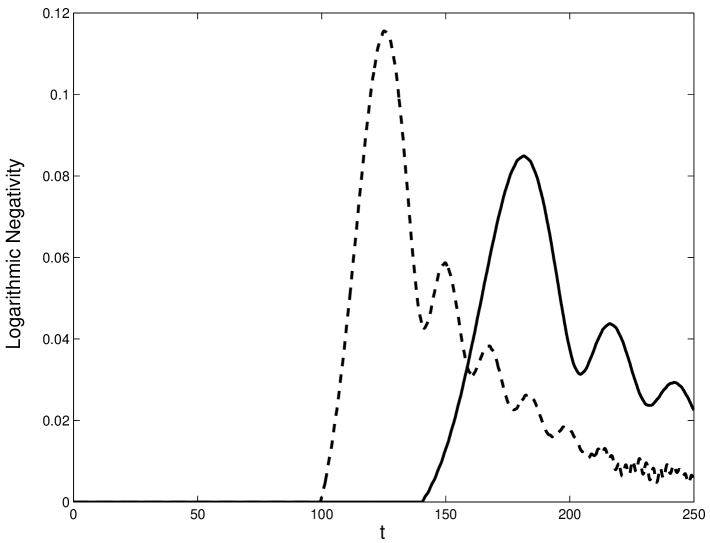
Figure 1: The time evolution of entanglement between the first and the last oscillator in an open chain of length $30$ when all the oscillators are initially in the ground state. The coupling strength $c=0.1$ has been chosen for the solid line ($c=0.15$ for the dashed line).

We observe no entanglement for a finite time until at a time $t_{0}$ one first encounters a build-up of entangled between the two oscillators. This time $t_{0}$ is approximately given by

$$t_{0}\cong\frac{n}{2\Omega\zeta},$$ (98)

ie the time $t_{0}$ is approximately linear in $n$, the separation of the oscillators. It should be noted that $t_{0}$ is half as large as the time that is required for a perturbation at the first oscillator to travel to the $n$-th oscillator. This suggests that the origin of the entanglement between the $1^{st}$ and the $n$-th oscillator arises from the interaction of those oscillators exactly half-way in between. Their entanglement is generated by the initial sudden switching on of the interaction and then propagates through the chain. This idea will be further corroborated in the later subsections when the propagation of pre-prepared entanglement is considered. Furthermore one finds that the dependence of the maximal degree of entanglement as measured by the logarithmic negativity is approximately proportional to $n^{-1/3}$ for large $n$ until reaches values of about $10^{-2}$ when it begins to drop quite rapidly to vanish entirely. It should be noted that for any parameters of the model there exists a finite $n$ such that the state of the first and the $n$-th oscillator is separable for all times. For the coupling value of $c=0.1$ this will happen for $n\cong 20000$. Therefore, the value of largest separation is very large indeed for reasonable coupling strengths. To appreciate that this is a somewhat surprising behaviour, it should be contrasted with the entanglement structure in the ground state of the chain. Then it can be shown that for any chosen coupling strength two distinguished oscillators are never in an entangled state, unless they are immediately neighbouring Audenaert EPW 02 .

Here we have studied the special case of the entanglement between the endpoint of an open chain. It should be noted that this is a particularly favourable configuration. For a given distance between oscillators one always obtains the largest amount of entanglement when one places them at the opposite ends of an open chain. Two oscillators in a very long chain with the same distance and with positions well away from the ends of the chain will lead to considerably smaller amounts of entanglement. Indeed, the amount of entanglement will differ by approximately a factor of $4$. This discrepancy is due to the fact that at the ends of the chain the oscillators possess fewer neighbours with which they can become entangled. As we discard all oscillators other than two any entanglement with other oscillators will deteriorate the entanglement between the distinguished oscillators. While this does not explain the factor of $4$ quantitatively, it gives an intuitive picture for the decrease of entanglement that will discussed in more detail later on.

V.2 Thermal state case

In the previous section we have studied the entanglement dynamics in an environment that is at zero temperature. This is reflected by the fact that the initial state of our harmonic oscillators is assumed to be the vacuum. We will now move one step further towards a more realistic description by setting the initial state as a thermal equilibrium state. As with the ground state case, we do not establish entanglement for the $H_{\rm RWA}$ interaction as a thermal state can be represented as a mixture of displaced vacuum states which do not lead to any spontaneous entanglement in the rotating wave approximation. Therefore we shall again only consider the $H_{\rm Spring}$ interaction. The thermal equilibrium state is given by

$$\gamma_{q_{n}q_{m}} = \delta_{nm}\Bigl{(}1+\frac{2}{e^{\omega/T}-1}\Bigr{)},$$ (99)

$$\gamma_{q_{n}p_{m}} = 0,$$

$$\gamma_{p_{n}p_{m}} = \delta_{nm}\Bigl{(}1+\frac{2}{e^{\omega/T}-1}\Bigr{)}.$$

The equations of motion are then

$$\gamma_{q_{n}q_{m}}(t) = \Bigl{(}1+\frac{2}{e^{\omega/T}-1}\Bigr{)}(a_{nm}(t)+d_{nm}(t)),$$ (100)

$$\gamma_{q_{n}p_{m}}(t) = \Bigl{(}1+\frac{2}{e^{\omega/T}-1}\Bigr{)}(b_{nm}(t)+e_{nm}(t)),$$

$$\gamma_{p_{n}p_{m}}(t) = \Bigl{(}1+\frac{2}{e^{\omega/T}-1}\Bigr{)}(c_{nm}(t)+a_{nm}(t)).$$

Appropriate values for the temperatures have to be obtained from experiment in the particular context under consideration, but it appears possible nowadays to achieve ratios $T/\omega\ll 1$ in different physical systems (note that we have taken $\hbar=1$ and $k=1$) such as nano-mechanical oscillators. We consider again an open chain instead of a closed ring. This renders the analytical treatment more difficult but makes no difference for the numerics. The entanglement depends little on the temperature as long as the mean thermal photon number is well below unity. Figure 2 shows the temperature dependence of entanglement evolution.

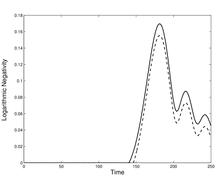
Figure 2: The time evolution of entanglement between the first and the last oscillator (with open boundary conditions). We have fixed $c=0.1$, the chain consists of $30$ oscillators, and $x=\omega/T$ for $x\geq 10$ (solid line) and $x=6$ (dashed line).

We observe that down to temperatures corresponding to $x=10$, the entanglement evolution is almost exactly the same as in the ground state case. Only when $x<10$ do we see an effect of a finite temperature. Even for $x=6$, we still have a significant portion of entanglement albeit a small delay in the arrival of entanglement. A more realistic scenario is dealt with in Ref. Eisert PBH 03 .

Decoherence mechanisms may be included without leaving the harmonic setting. Often, the high temperature limit of Ohmic quantum Brownian motion is appropriate with an independent heat bath for each oscillator in the limit of negligible friction and under the assumption of product initial conditions. Such a decoherence mechanism can be accounted for by adding terms of the form Giulini JKKSZ 96 ; Zurek 03

$$-\xi[\hat{q}_{n},[\hat{q}_{n},\rho]]$$ (101)

to the idealized unperturbed generator of the dynamical map for each of the oscillators, where the real number $\xi$ specifies the decoherence time scale. However, in cases where product initial conditions are inappropriate or unrealistic, decoherence may still be modeled using, for example, time-convolutionless projection operator techniques Breuer P 02 . In small systems, non-product conditions may be incorporated by explicitly appending heat baths to each of the oscillators with a linear coupling Zuercher T 90 , according to Hamiltonians of the form

$$\hat{H}_{n}=\Biggl{(}\hat{q}_{n}\otimes\sum_{i=1}^{m}\xi_{j}\hat{q}_{j}^{(i)}\Biggr{)}$$ (102)

with real numbers $\xi_{j}$, where the $\hat{q}_{j}^{(i)}$ denote the canonical coordinates corresponding to position of the $i$-th oscillator of the $j$-th heat bath consisting of $m$ oscillators. Assuming a particular form of the spectral density, the coupling strength to the finite heat baths may be chosen in a way that is consistent with empirically known values for energy dissipation. Often, $Q$-factors are approximately known for resonators, which quantify the number of radians of oscillations necessary for the energy to decrease by a factor of $1/e$. Hence, on the basis of these $Q$-factors, the appropriate coupling may be evaluated. Figure 3 shows the influence of decoherence in case of an open chain with the same parameters as in Figure 1 for an Ohmic heat bath, i.e., $\xi_{j}=j\Lambda/m$, where $\Lambda>0$ is the cut-off frequency of the environment modes. One finds that the created entanglement by suddenly switching on the interaction is surprisingly robust against decoherence within this model.

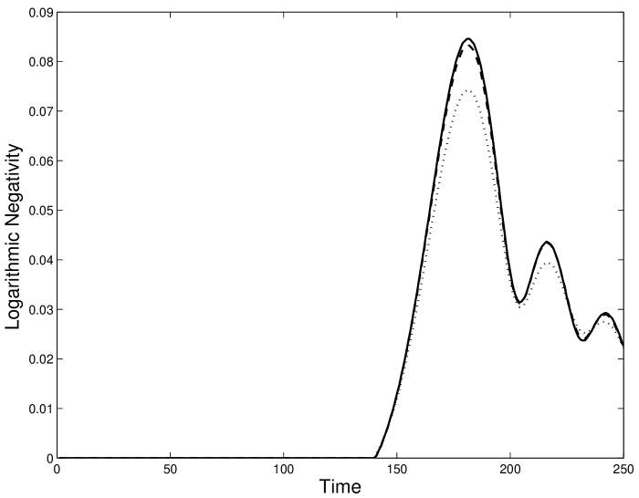
Figure 3: The same as Figure 1, without Ohmic dissipation and decoherence (solid line), and with Ohmic dissipation corresponding to $Q=10000$ (dashed line) and $Q=1000$ (dotted line).

V.3 Entanglement transport through the harmonic chain

In the previous section we considered the case where no entanglement was present in the initial state of the system. Entanglement emerged as a consequence of a sudden change in the coupling constant between neighbouring harmonic oscillators. In this subsection we are going to investigate a different situation and consider the transmission of entanglement through a one dimensional chain. To this end we initialise two harmonic oscillators in a two mode squeezed state. We assume that one of these oscillators is decoupled from the rest and give it the index $0$, while the other oscillator, with index $1$, forms part of a chain of harmonic oscillators with nearest neighbour interaction. The remainder of the chain starts out in the ground state corresponding to zero temperature (assuming no interactions). By evolving the initial state, we expect the entanglement to travel along the chain so that with increasing time more and more distant oscillators will be entangled with the $0$-th harmonic oscillator. There are a number of free parameters that can be varied: the coupling strength $c$, the amount of initial entanglement quantified by the two-mode squeezing parameter $r$, the time $t$ and the position of the oscillator to be entangled with the $0$-th oscillator. In order to simplify the analytical work, we shall be dealing with the limit $M\rightarrow\infty$.

While in the previous section the interaction in the rotating wave approximation does not lead to the spontaneous creation of entanglement, here it allows for the propagation of entanglement. We give an example for the time evolution of the logarithmic negativity between the $0$-th and the $30$-th oscillator for both interactions in Figure 4.

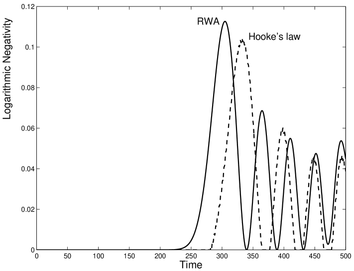
Figure 4: The time evolution of entanglement between the $0$-th and the $30$-th oscillator in a chain with 80 oscillators with periodic boundary conditions. We have chosen $c=0.1$ and $r=0.8$ in both cases. The entanglement propagates slightly faster in the rotating wave interaction.

For both interactions we obtain qualitatively the same behaviour but we observe that under the RWA interaction the entanglement propagates somewhat faster but as expected this difference decreases with decreasing coupling constant $c$. Another difference is the fact that the entanglement under the RWA interaction does not exhibit the small-amplitude oscillations that the interaction due to harmonic oscillators coupled by springs exhibits due to the existence of counter-rotating terms of the form $\hat{a}_{k}\hat{a}_{k+1}$. The propagation of the quantum entanglement can be seen even more clearly in Figure 5 where for a ring composed of $40$ oscillators and a coupling constant of $c=0.1$ the time evolution of the logarithmic entanglement between an uncoupled oscillator and the $n$-th oscillator is shown when initially the uncoupled oscillator and the $1$-st oscillator are coupled. One observes that with increasing time more and more distant oscillators are becoming entangled. Entanglement propagates both clockwise and anti-clockwise around the ring. After a sufficiently long time it becomes important that the ring has a finite size and the two counter-rotating ’entanglement waves’ meet at the opposite end of the ring and we observe some entanglement enhancement.

Figure 5: For a ring of $40$ oscillators and a coupling constant of $c=0.1$ the time evolution of the logarithmic entanglement between an uncoupled oscillator and the $n$-th oscillator is shown when initially the uncoupled oscillator and the $1$-st oscillator are in a two-mode squeezed state with two-mode squeezing parameter $r=0.8$. With increasing time more and more distant oscillators are becoming entangled. Entanglement propagates both clockwise and anti-clockwise around the ring. After a sufficiently long time the two counter-propagating ’entanglement waves’ meet at the opposite end of the ring and we observe some entanglement enhancement.

Both Figures 4 and 5 suggest that entanglement can be distributed to distant oscillators. It will therefore be interesting to study the efficiency for this transfer when we vary the amount of entanglement provided initially by varying $r$. In particular, we will be interested in the first local maximum in the amount of entanglement $N_{f}$ as quantified by the logarithmic negativity.

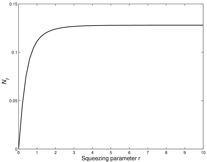
Figure 6: For oscillators interacting by springs the graph shows the amount of entanglement at the first local maximum as squeezing is varied. We have fixed $c=0.1$ and $n=30$.

We separate the study of the entanglement transfer efficiency for the two interactions as they exhibit distinctly different behaviours. We begin with the interaction describing oscillators interacting via springs. Figure 6 shows the amount of entanglement at the first local maximum as squeezing is varied. We observe the remarkable fact that for large initial entanglement, the value of $N_{f}$ saturates. We can obtain an analytic expression for the saturation value as a function of $c$ and $n$ by taking the $r\rightarrow\infty$ limit. Thus, we approximate $\eta_{\rm Spring}^{2}\cong-w/(8y_{1})$ of Eq. (75) and, discarding all the terms except $\cosh^{2}(r)\cong e^{2r}/4$ and $\cosh(2r)\cong e^{2r}/2$, we obtain

$$\eta_{\rm Spring}^{2}\cong\frac{\left(-2J^{2}_{\rm max}+(1+4c)^{-1/2}+1\right)\left(-J^{2}_{\rm max}+c+1\right)}{2\left(J^{2}_{\rm max}+1\right)^{2}},$$ (103)

where $J_{\rm max}=0.6748851(n-1)^{-1/3}$ olver is the value of the first maximum of the $n$-th Bessel function of the first kind. This substitution provides a very good approximation as the first local maximum of the logarithmic negativity coincides with that of the $n$-th Bessel function. Therefore we find $N_{\rm sat}=-\log_{2}(|\eta_{\rm Spring}|)$ which is shown in Figure 7.

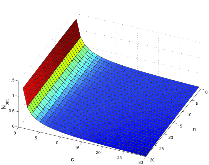
Figure 7: A graph to show how the saturation value $N_{\rm sat}$ for the logarithmic negativity varies with the coupling strength $c$ and the position $n$ of the second oscillator.

We observe that the saturation value decreases for both increased coupling strength and increased distance. While the latter is intuitive the former might be surprising as one could have thought that it is advantageous to increase the coupling strength to facilitate the transfer of entanglement but this intuition is clearly contradicted by Figure 7. Even more strikingly the entanglement vanishes entirely when the interaction strength becomes too high. We believe that this is due to the fact that the initial entanglement disperses across several oscillators and will discuss this at the end of this subsection.

If we translate these findings into an entanglement transfer efficiency defined by

$$T_{\rm eff}=\frac{N_{f}}{N_{i}},$$ (104)

then we observe that this efficiency exhibits a non-monotonic behaviour. Indeed, we observe a maximum in the efficiency as shown in Figure 8 for the same parameters as in Figure 6. We have not yet found a convincing and intuitive explanation for the occurrence of a maximum in the transfer efficiency nonmonotonic . In fact we will shortly see that the phenomenon of a non-monotonic transfer efficiency is absent in the RWA interaction. The surprising implication of this non-monotonic behaviour of the transmission efficiency is that it is advantageous to transmit entanglement in intermediate size portions rather than in one very large packet.

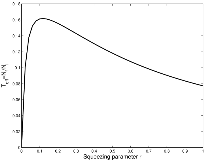
Figure 8: The efficiency of transmission as squeezing is varied for $c=0.1$ and $n=30$. Surprisingly, the transmission efficiency exhibits a maximum at a finite initial entanglement.

Let us now consider the same problem of the entanglement transfer efficiency in the RWA interaction. Indeed, we can show that there is still saturation in the amount of entanglement that can be transmitted and we find the value of the saturation to be (after taking $r\to\infty$)

$$N_{\rm sat}=-\log_{2}\left(\frac{1-J_{\rm max}^{2}}{1+J_{\rm max}^{2}}\right),$$ (105)

where again $J_{\rm max}=0.6748851(n-1)^{-1/3}$ olver is the value of the first maximum of the $n$-th Bessel function of the first kind. Note that this expression is independent of the coupling strength $c$. Unlike the case of oscillators interacting with springs there is no maximum in the efficiency for the RWA interaction as can be seen clearly in Figure 9. Indeed, for large $r$ the efficiency is tending to zero while for $r$ approaching $0$ the efficiency tends to $T_{\rm eff}=J_{\rm max}$.

Since the efficiency is not equal to unity for both interactions, the question arises as to where the rest of the entanglement is located? The most obvious place is to search in the neighbourhood of the $n$-th oscillator. Since we always determine the entanglement between individual oscillators we ignore many others that have interacted with it and have thereby become entangled. Any entanglement between these two oscillators will therefore deteriorate as they are being entangled with other oscillators that we choose to ignore. This viewpoint is corroborated by determining the entanglement between the $0$-th oscillator and a whole group of neighbouring oscillators instead of a single one. The result of this can be seen in Figure 10.

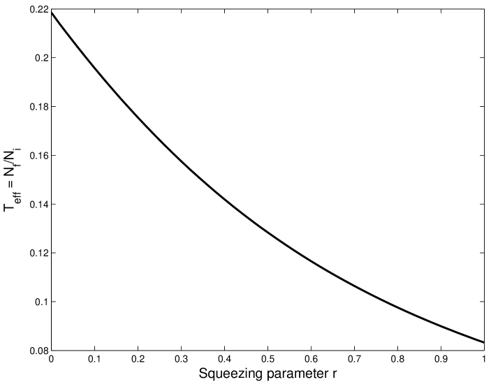
Figure 9: The efficiency of the RWA interaction versus the two-mode squeezing parameter $r$, $n=30$ and $c=0.1$.

This shows the change in the amount of entanglement as we increases the number of oscillators in the second group. The graph supports the idea that the missing entanglement between the $0$-th and the $n$-th oscillator is due to the creation of entanglement between the $n$-th oscillator and its neighbours because we start to recover entanglement as we compute the entanglement between the $0$-th oscillator and the neighbourhood of oscillators surrounding the $n$-th oscillator. This spread of entanglement is not dissimilar to a dispersion of the energy of a wavepacket as it experiences different group velocities. However, the effect on the entanglement can be considerably stronger as the energy will only decrease linearly with the width of the wave-packet while the entanglement can drop much more rapidly and become zero at finite spreading.

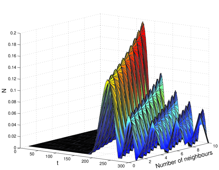
Figure 10: The change in the amount of entanglement as the number of oscillators of system $B$ centered around the $20$-th oscillator is increased from $n_{2}=1$ to $n_{2}=21$. We have a ring of 70 oscillators with squeezing parameter $r=0.8$. Increasing the number of neighbours increases the amount of entanglement available. This supports the idea that the loss of entanglement is due to dispersion.

V.4 Speed of entanglement propagation

We have found that the propagation of half the two mode squeezed state through the chain takes a finite time as the entanglement between the $0$-th and the $n$-th oscillator is exactly zero for a finite time interval (see for example Figure 4). After a certain amount of time, the two oscillators in question become entangled and the logarithmic negativity reaches a temporary maximum. We are able to determine this time analytically for both types of interactions that we are considering. To make the analysis tractable, we consider an infinitely long chain. We find that the first maximum of the logarithmic negativity coincides with the first maximum of a Bessel function $J_{m}(x)$. We know the position of this maximum occurs at $x=m+0.8086165m^{1/3}$ olver . Noting that $m=n-1$, $x=\zeta\Omega t=ct/\sqrt{1+2c}$ for the Hooke’s law interaction and $x=ct$ in the RWA interaction, we obtain

$$t_{\rm Spring} = \frac{n-1+0.8086165(n-1)^{1/3}}{\zeta\Omega},$$ (106)

$$t_{\rm RWA} = \frac{n-1+0.8086165(n-1)^{1/3}}{c}\,.$$

We observe that the time that is required for entanglement to be established between the $0$-th and the $n$-th oscillator is a function of the coupling strength and the position $n$. For large separations $n$, it quickly becomes linear in $n$ and as expected, the larger the coupling $c$ the faster entanglement is established. We also see that the RWA interaction produces faster entanglement since $t_{\rm Spring}/t_{\rm RWA}=\sqrt{1+2c}$. As $n-1$ is the separation of the $1$-st and the $n$-th oscillator we can define the speed of propagation to be

$$v_{\rm Spring} = \frac{c}{\sqrt{1+2c}\left(1+0.8086165(n-1)^{-2/3}\right)}\cong\frac{c}{\sqrt{1+2c}},$$

$$v_{\rm RWA} = \frac{c}{1+0.8086165(n-1)^{-2/3}}\cong c.$$ (107)

Clearly, for large $n$, the speeds approach a constant dependent on $c$. For the RWA interaction, the propagation velocity increases linearly with $c$. This is an attractive feature because unlike the case of interaction via springs, the efficiency under the rotating wave approximation does not decrease as we increase $c$ because its efficiency is independent of $c$.

V.5 Optimization of entanglement transfer and generation

In the previous section we have studied the entanglement transfer along a chain of identical harmonic oscillators as this will be the situation that is most easily implemented experimentally. However, we observe that the transmission efficiency decreases with distance. One might expect that one can improve this efficiency by tuning the couplings and the eigenfrequencies of the harmonic oscillators suitably. Indeed, in this section we will show what can be achieved in this more general setting. For simplicity we consider the task of transmitting one half of a two-mode squeezed state from one end of an open chain to the other.

We assume as usual one decoupled harmonic oscillator with index $0$ and a chain of length $M$ through which the other half of the two-mode squeezed state is transmitted. Perfect transmission from one end of the chain to the other is possible in the rotating-wave interaction of nearest neighbours if we choose the interaction strength

$$V_{n,n+1}=V_{n+1,n}=c\sqrt{n(M-n)}$$ (108)

and

$$V_{n,n}=1,$$ (109)

with the real number $c$ being sufficiently small in order for $V$ to be positive. The choice of the diagonal elements being all equal to $1$ is equivalent to the requirement that we choose the eigen-frequencies $\omega_{n}$ of the uncoupled oscillators as

$$\omega_{1} = 1-c\sqrt{(M-1)},$$ (110)

$$\omega_{n} = 1-c\sqrt{n(M-n)}-c\sqrt{(n-1)(M-n+1)}\,.$$

That the transmission is perfect can be shown by first realizing that in an interaction picture with respect to $H_{0}=\sum_{i}(\hat{q}_{i}^{2}+\hat{p}_{i}^{2})/2$ in which the diagonal elements of $V$ vanish (this interaction picture will leave all entanglement properties unaffected as it is of direct sum form) we can replace

$$\left[\begin{array}[]{c}Q(t)\\ P(t)\\ \end{array}\right]=\exp\left({\left[\begin{array}[]{cc}0&V_{I}\\ -V_{I}&0\\ \end{array}\right]t}\right)\left[\begin{array}[]{c}Q\\ P\\ \end{array}\right],$$ (111)

where $Q$ and $P$ are column vectors, by the complex notation $Q-iP$ so that

$$(Q-iP)(t)=e^{iV_{I}t}(Q-iP)\,.$$ (112)

Now we need to realize that $V_{I}$ is a quantum mechanical representation of a rotation. This allows the evaluation of the matrix elements of $e^{iV_{I}t}$. In particular, we find that

$$(e^{iV_{I}t})_{1M}=\left(\sin(ct/2)\right)^{M-1},$$ (113)

so that one can generate an interchange between the first and the $M$-th coordinate by waiting for a time $t=\pi/c$ (see Ref. Christandl DEL 03 for an analogous argument in spin chains).

Without the assumption of the rotating wave approximation, i.e., choosing the Hamiltonian $H_{\rm Spring}$ to describe the time evolution the above simple argument fails and indeed it is not possible to tune the nearest neighbour couplings alone to generate perfect transfer of entanglement for $M>2$. However, if one chooses the couplings as above and decreases the value of the constant $c$ then, for a fixed distance, one can obtain arbitrarily good transfer efficiency at the expense of an increased delay time. This should not come as a surprise, as in the case of $c\rightarrow 0$ the rotating wave approximation becomes exact as the terms that are neglected in the rotating wave approximation are of order ${\cal O}(c^{2})$. Therefore, for entanglement distribution over a fixed distance they will play a decreasing role as the time of arrival for the entanglement is of the order ${\cal O}(c^{-1})$.

The case $M=2$ is an exception, where one may realize an exact swap of the state of the $1$-st to the $2$-nd oscillator. To show this, note that specific covariance matrix elements of the $0$-th and the $2$-nd oscillator are given by

$$\gamma_{p_{0}p_{2}}(t) =-\sinh(r)f_{1}(t),\,\,\,\,\gamma_{q_{0}q_{n}}(t) =\sinh(r)f_{1}(t),$$ (114)

$$\gamma_{q_{0}p_{2}}(t) =\sinh(r)\dot{f}_{1}(t),\,\,\,\,\,\,\,\,\,\,\,\gamma_{q_{2}p_{0}}(t) =-\sinh(r)g_{1}(t).$$

Considering the functions $f_{1}$ and $g_{1}$ as specified in eqs. (39), we find that there exists a real number $c$ and a time $t$ such that simultaneously

$$f_{1}(t)=1,\,\,\,\,\,\,\,\,\,\,\,\dot{f}_{1}(t)=0,\,\,\,\,\,\,\,\,\,\,\,g_{1}(t)=0$$ (115)

can be satisfied. This is the case when we chose the real $c$ such that there exist natural numbers $k$ and $l$ such that

$$c=\left(\frac{(2k+1)^{2}}{l^{2}}-1\right)/4$$ (116)

and $t=l\pi$. Then, it follows that, as the $0$-th oscillator is invariant and the state of the $0$-th and the $2$-nd oscillator necessarily corresponds to a pure Gaussian state, the $1$-st oscillator is necessarily decoupled from the other two. In this sense the state can be swapped from one oscillator to the other, while retaining the entanglement with the $0$-th oscillator. Hence, one has a perfect channel for appropriate times.

V.6 Sensitivity to random variations in the coupling

In the preceding subsections we have discussed an ideal model in which all experimental parameters can be determined perfectly. Any real experimental setup however will suffer small variations in parameters such as the coupling strength between neighbouring oscillators. In order to confirm that the effects that have been found in this work can be observed in real experiments, we consider in the following the impact of random position dependent variations in the coupling strength between neighbouring oscillators. As an example, we consider an open chain with potential matrix

$$V=\left[\begin{array}[]{ccccccc}1&0&0&0&\cdots&0&0\\ 0&1+c_{1,2}&-c_{1,2}&0&\cdots&0&0\\ 0&-c_{1,2}&\ddots&\ddots&&&0\\ 0&0&\ddots&1+c_{i-1,i}+c_{i,i+1}&-c_{i,i+1}&0&\vdots\\ \vdots&\vdots&&-c_{i,i+1}&1+c_{i,i+1}+c_{i+1,i+2}&\ddots&0\\ 0&0&&&\ddots&\ddots&-c_{n-1,n}\\ 0&0&0&\cdots&0&-c_{n-1,n}&1+c_{n-1,n}\end{array}\right],$$ (117)

where $c_{i,j}=c+\Delta c_{i,j}$ is the position dependent coupling between the $i$-th and $j$-th oscillators, where $\Delta c_{i,j}$ is a realization of a random variable distributed according to a normal $N(0,\Delta c)$ distribution. For a chain of length $10$, an average coupling constant of $c=0.1$ and an initial two mode squeezed state with squeezing parameter $r=0.8$. Figure 11 shows the ratio of the first maximum for the case of slightly perturbed couplings over the idealized case versus the perturbation size $\Delta c$.

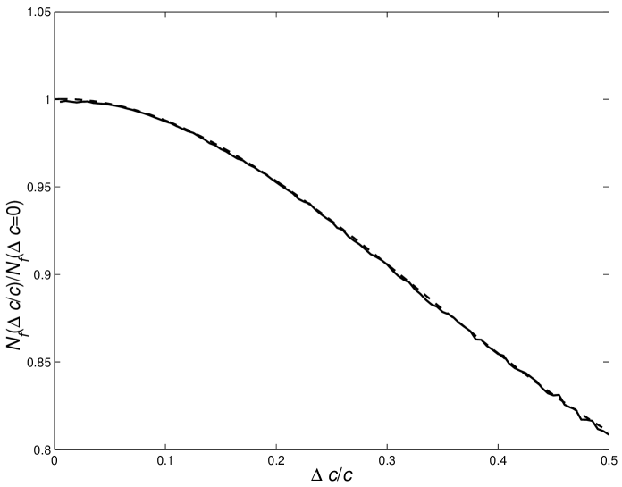
Figure 11: The ratio of the first maximum for the case of slightly perturbed couplings over the idealized case versus the relative perturbation size $\Delta c/c$ for a chain of length $30$, $r=0.8$ and $c=0.1$. Each data point has been obtained as an average over 4000 realizations. The resulting curve is very well fitted by the function $f(\Delta c/c)=1+0.02382\Delta c/c-1.60481(\Delta c/c)^{2}+1.59676(\Delta c/c)^{3}$.

We observe that for $\Delta c/c\leq 0.25$, the achieved entanglement is greater than $95\%$ of the degree of entanglement in the unperturbed case. Similar results apply for the RWA interaction. These results indicate that sending quantum information along the chain is stable under perturbations.

Similar considerations can be made for the spontaneous creation of entanglement which show that the results are much more sensitive to perturbations. Indeed, with the same specifications as above we find the entanglement at the first maxima to be between a small fraction and twice the amount for the non-perturbed case when $\Delta c/c=0.5$. This suggests that the experimental demands for the verification of the spontaneous creation of entanglement are considerably higher than for the distribution of entanglement.

V.7 Other geometrical arrangements: Beamsplitters and interferometers

So far we have studied only a linear chain of harmonic oscillators through which quantum entanglement can be propagated. However, it might be interesting to consider more complicated structures which may be used as building blocks for more complicated networks, in principle, any arrangement corresponding to an arbitrary weighted graph.

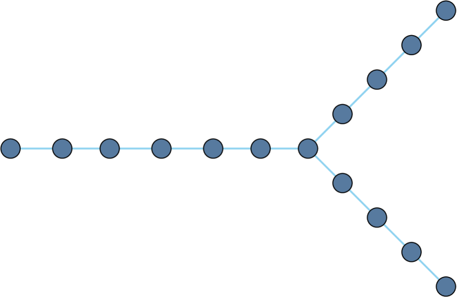
Figure 12: This figure depicts a Y-shaped structure as it is described in the text. A single incoming arm consists of $M_{\rm in}$ oscillators (here $7$) is connected to two outgoing arms each consisting of $M_{\rm out}$ oscillators (here $4$).

In this subsection we will study briefly two possible extensions of the linear chain, namely a Y-shaped configuration which can be used for the generation of entanglement and a configuration resembling an interferometer. We show furthermore how such configurations may be switched on and off thereby controlling the transport of quantum information in such a structure. A more detailed discussion of such structures and their optimization will be presented elsewhere. The material in this subsection should merely serve as examples for possible alternative ways of creating and manipulating entanglement through propagation in pre-fabricated structures.

We begin by considering a chain in Y-shape which is shown in Figure 12. One arm consisting of $M_{\rm in}$ oscillators is connected to two further arms each consisting of $M_{\rm out}$ oscillators. As usual we consider nearest neighbour interactions only and, for simplicity and the clearest demonstration of the effects, we restrict attention to the RWA interaction. We assume that the structure is initially in the ground state, i.e., at temperature $T=0$. At time $t=0$ we perturb the first harmonic oscillator exciting it either to a thermal state characterized by covariance matrix elements

$$\gamma_{q_{1}q_{1}}=\gamma_{p_{1}p_{1}}=z$$ (118)

for some $z$, or a pure squeezed state characterized by covariance matrix elements

$$\gamma_{q_{1}q_{1}}=1/\gamma_{p_{1}p_{1}}=z\,.$$ (119)

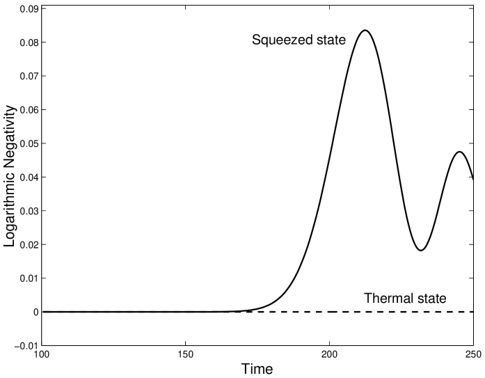
Figure 13: In a chain with Y-shape and nearest neighbour interaction of RWA type the first oscillator at the foot of the Y-shape is either excited to a squeezed state with $\gamma_{qq}=10=1/\gamma_{pp}$ or a thermal state with $\gamma_{qq}=10=\gamma_{pp}$. The remaining oscillators are in the ground state. The perturbation propagates along the chain into both arms of the Y-shape. For an initial thermal state excitation no entanglement is ever found between the ends of the two arms of the Y-shape while entanglement is generated when the initial state is a squeezed state. The coupling constant is chosen as $c=0.2$, the arms of the Y-shape contain $30$ oscillators each while the base contains $10$ oscillators.

As an example we choose a coupling constant of $c=0.2$ and let the arms of the Y-shape contain $M_{\rm out}=30$ oscillators each while the base contains $M_{\rm in}=10$ oscillators. In Figure 13 we present the results for the choice of a squeezed state with $\gamma_{q_{1}q_{1}}=10=1/\gamma_{p_{1}p_{1}}$ and a thermal state with $\gamma_{q_{1}q_{1}}=10=\gamma_{p_{1}p_{1}}$.

We observe that for an initial thermal state excitation no entanglement is ever found between the ends of the two arms of the Y-shape. This can be understood because a thermal state is a mixture of coherent states, i.e., displaced vacuum states. If the system is initialized in the vacuum state it will evidently not lead to any entanglement in the RWA and therefore an initialization in a thermal state cannot yield entanglement either. On the other hand considerable entanglement is generated when the initial state is a squeezed state. It is possible to optimize the generation of entanglement by adjusting the strength of the nearest neighbour couplings but this will be pursued elsewhere. These two observations are resembling closely optical beamsplitters which do not create entanglement from thermal state input but can generate entanglement from squeezed inputs (see Ref. Wolf EP 03 for a comprehensive treatment of the entangling capacity of linear optical devices).

Another interesting setup is shown in Figure 14. We will henceforth call this the interferometric setup. Let the number of oscillators on the left (including the junction), up arm, down arm and on the right be $M_{L}$, $M_{U}$, $M_{D}$ and $M_{R}$ respectively.

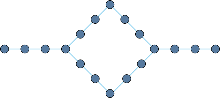
Figure 14: A diagram of the interferometric setup.

If we prepare a two-mode squeezed state between a decoupled oscillator and the leftmost oscillator of the interferometric setup, then we are interested in how much entanglement propagates through the setup depending on the properties of the two arms. One may vary different parameters such as the length of one of the arms, the coupling strength or eigenfrequency of the oscillators in one arm. We will focus on how the change in eigenfrequency $\omega$ of the harmonic oscillators in one of the arms affects the propagation of entanglement through the interferometric device. We change the eigenfrequencies of the oscillators smoothly across one arm following $\omega_{i}=1+(\omega-1)\times\min(i,M_{U}+1-i)/(M_{U}/2)$ so that the oscillator half way through the arm has frequency $\omega$. Figure 15 shows the logarithmic negativity between the decoupled oscillator and the last one in the interferometric configuration at the time $t=250$ plotted against $\omega$. The other parameters are $M_{U}=M_{D}=30$, $M_{L}=M_{R}-1=9$ and $c=0.2$. One clearly observes interference fringes in the frequency $\omega$ that are related to the effective path-length difference between the upper and the lower arm. The interference fringes do not have full amplitude and their amplitude is reduced for increasing $\omega$. More sophisticated choices for the coupling parameters in the interferometric structure can improve on these imperfections. This demonstrates that in interferometric structure the transmission through the device will be strongly influenced by changes of the properties of one arm of the structure.

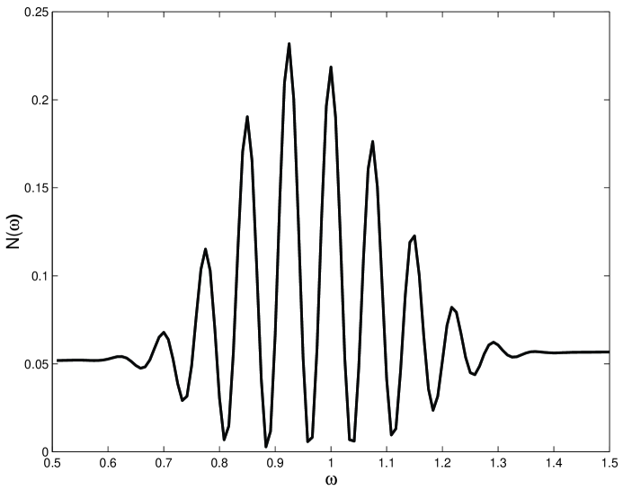
Figure 15: The logarithmic negativity $N(\omega)$ between the decoupled oscillator and the last one in the interferometric configuration at the time $t=250$ plotted against $\omega$. We have chosen $M_{L}=M_{R}-1=9$, $M_{U}=M_{D}=30$ and $c=0.2$ in the RWA interaction. One clearly observes interference fringes.

This shows that more complicated structures such as the Y-shape or the interferometric may be used to create entanglement from an initially unentangled system and transport it. There is a distinct analogy here to quantum optical networks which might be used for information processing either employing the polarization degree of freedom or as we did here the excitation number degree of freedom. This suggests that one could construct similar ’hardwired’ networks on the level of interacting quantum systems that could then perform certain quantum information processing or communication tasks. This might involve structures such as the Y-shape presented here but may also implement structures such as interferometer structures shown in Figure 14 or multi-input devices.

If one were to consider hardwired structures, then it would be necessary to devise methods by which these structures could be switched on and off. Here we explore two possibilities. Firstly, one might change the coupling strength $c_{\rm Junction}$ of the oscillator at the three way junction in the Y-shape. Apart from the obvious fact that they remain disentangled for $c_{\rm Junction}=0$ (i.e., uncoupled), we find the first maximum for the entanglement decreases to roughly half the value for large coupling strength $c_{\rm Junction}=0.8$. This is shown in Figure 16. A further increase of the coupling strength to $c_{\rm Junction}=5$ does not lead to further significant change.

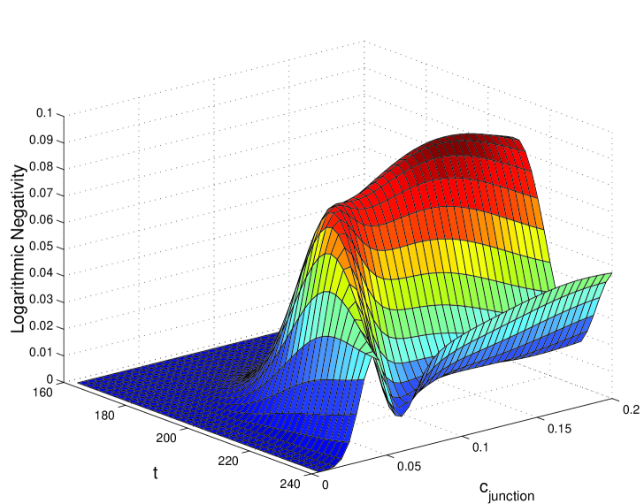
Figure 16: The degree of entanglement in the Y-structure in terms of the coupling strength $c_{\rm Junction}$ of the oscillator at the three-way junction. The parameters are chosen identically as in Figure 13.

A different approach would be to change the eigenfrequency or the mass of the junction oscillator while keeping the coupling strength the same as the other oscillators. Indeed, if we increase the eigenfrequency $\omega_{\rm Junction}$, the entanglement can be reduced to an arbitrarily small amount for both RWA and spring-interactions. A decrease of the eigenfrequency is less efficient but would also allow a significant reduction of the amount of entanglement generated in the device. Figure 17 demonstrates these effects achieved by changing the eigenfrequency of the junction oscillator in the Y-shape. It should be noted that the dependence of the logarithmic negativity with the eigenfrequency $\omega_{\rm Junction}$ is almost perfectly fitted by a Lorentzian line shape.

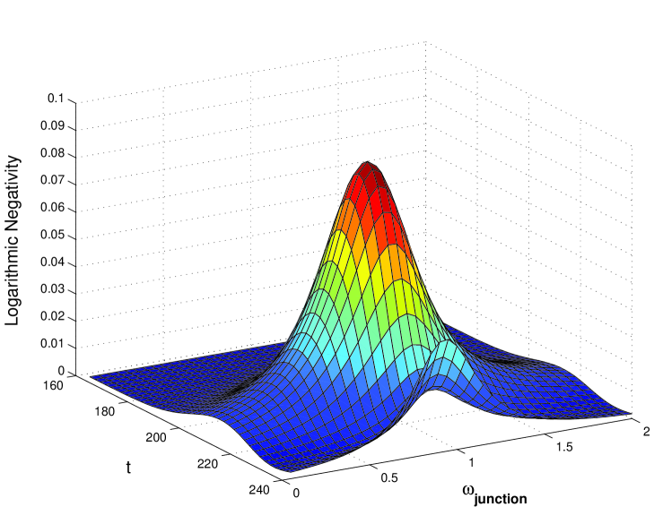
Figure 17: By increasing and decreasing $\omega_{\rm Junction}$ respectively in the Y-shape we observe a noticeable change in the amount of entanglement that is generated in the device. The other parameters are chosen as in Figure 13.

The above examples suggest, that it is possible to switch on and off pre-fabricated devices such as the Y-shape shown above by adjusting either the coupling strength (decreasing it, i.e., approach decoupling) or the eigenfrequency (increasing it). Such a manipulation of the junction oscillator dictates the quantum information flowing through the junction. An example for a possible implementation of such a switch from an optical setting would be coupled optical cavities which are filled with atoms. Laser irradiation of these atoms would then lead to a shift of the resonance frequency of the cavity which corresponds to a change in the eigenfrequency of a harmonic oscillator in the above examples. In this way, individual cavities might be decoupled. A detailed study of such a scheme will be presented elsewhere. Finally, we would like to briefly mention an analogy with the monotonic and non-monotonic behaviour of the efficiency. We find that by increasing the mass of the junction oscillator in the beamsplitter configuration, we obtain monotonically decreasing entanglement between the two ends for the RWA interaction whereas the Hooke’s law interaction produced non-monotonic behaviour.

VI Conclusions and Discussions

We have investigated the entanglement dynamics of systems of harmonic oscillators both analytically and numerically. Particular attention has been paid to harmonic oscillators coupled by springs (Spring) and to harmonic oscillators with a linear coupling in a rotating wave approximation (RWA) as it is appropriate in a quantum optical setting. After an introduction to the mathematical formalism and the derivation of the analytical solutions for the equations of motion for these interactions we then investigated several possible scenarios. We considered the generation of entanglement without detailed local control of individual systems. This was achieved by first switching off any interaction between the oscillators, cooling them to near the ground state and subsequently switching on the coupling suddenly. Surprisingly, entanglement will be generated over very large distances which is in stark contrast to the entanglement properties of the stationary ground state of a harmonic chain where only nearest neighbours exhibit entanglement Audenaert EPW 02 . We have also demonstrated that a linear chain of harmonic oscillators is able to transport quantum information and quantum entanglement for various types of nearest neighbour coupling. For position independent nearest neighbour coupling we observe that the transmission efficiency is a non-monotonic function in the coupling strength for Hooke’s law coupling while it is monotonically decreasing for the RWA coupling. In both cases this suggests that it is advantageous to transmit entanglement in smaller portions rather than large units. But due to the rapid decline in efficiency with the spring interaction for very small $r$, one should avoid sending in too smaller $r$. The propagation speed for the quantum entanglement has been provided analytically. For the above effects we have studied their sensitivity to random variations in the coupling between the oscillators and to finite temperatures.

Finally we have proposed more complicated geometrical structures such as Y-shapes and interferometric setups that allow for the generation of entanglement in pre-fabricated structures without the need for changing any coupling constants. We have also shown that these structures may be switched on and off by changing the coupling of only a single harmonic oscillator with its neighbours. This suggests the possibility for the creation of pre-fabricated structures that may be ’programmed’ by external actions. Therefore quantum information would be manipulated through its propagation in these pre-fabricated structures somewhat analogous to modern micro-chips and as opposed the most presently suggested implementations of quantum information processing where stationary quantum bits are manipulated by a sequence of external interventions such as laser pulses.

All these investigations were deliberately left at a device independent level. It should nevertheless be noted that there are many possible realizations of the above phenomena. These include nano-mechanical oscillators Eisert PBH 03 , arrays of coupled atom-cavity systems, photonic crystals, and many other realizations of weakly coupled harmonic systems, potentially even vibrational modes of molecules in molecular quantum computing Tesch R 02 . A forthcoming publication will discuss device specific issues of such realization as well as well as improved structures (including novel topological structures as well as changes of their internal structure such as di-atomic chains) that allow for better performances with less experimental resources. We hope that these ideas may lead to the development of novel ways for the implementation of quantum information processing in which the quantum information is manipulated by flowing through pre-fabricated circuits that can be manipulated from outside.

We acknowledge discussion with D. Angelakis, S. Bose, D. Browne, M. Christandl, M. Cramer, J. Dreißig, J.J. Halliwell, T. Rudolph, M. Santos, V. Vedral, S. Virmani, and R. de Vivie-Riedle. This work was supported by the Engineering and Physical Sciences Research Council of the UK, the ESF programme ”Quantum Information Theory and Quantum Computing”, the EU Thematic Network QUPRODIS and the Network of Excellence QUIPROCONE, the US Army (DAAD 19-02-0161), the EPSRC QIP-IRC, and the Deutsche Forschungsgemeinschaft DFG. MBP is supported by a Royal Society Leverhulme Trust Senior Research Fellowship.

References

- (1) J.I. Cirac, P. Zoller, H.J. Kimble, and H. Mabuchi, Phys. Rev. Lett. 78, 3221 (1997).
- (2) L.-M. Duan and H.J. Kimble, Phys. Rev. Lett. 90, 253601 (2003).
- (3) X.L. Feng, Z.M. Zhang, X.D. Li, S.Q. Gong, Z.Z. Xu, Phys. Rev. Lett. 90, 217902 (2003).
- (4) D.E. Browne, M.B. Plenio and S.F. Huelga, Phys. Rev. Lett. 91 067901 (2003).
- (5) N. Khaneja and S.J. Glaser, Phys. Rev. A 66, 060301 (2002).
- (6) S. Bose, Phys. Rev. Lett. 91, 207901 (2003).
- (7) V. Subrahmanyan, LANL e-print quant-ph/0307135.
- (8) M. Christandl, N. Datta, A. Ekert, A.J. Landahl, LANL e-print quant-ph/0309131.
- (9) T. Osborne and N. Linden, LANL e-print quant-ph/0312141.
- (10) J. Eisert and M.B. Plenio, Int. J. Quant. Inf. 1, 479 (2003), LANL e-print quant-ph/0312071.
- (11) J. Eisert, M.B. Plenio, S. Bose and J. Hartley, LANL e-print quant-ph/0311113.
- (12) K. Audenaert, J. Eisert, M.B. Plenio, and R.F. Werner, Phys. Rev. A 66, 042327 (2002).
- (13) T.A. Brun and J.B. Hartle, Phys. Rev. D 60, 123503 (1999).
- (14) J.J. Halliwell, Phys. Rev. D 68, 025018 (2003).
- (15) M.L. Roukes, Phys. World 14, 25 (2001).
- (16) K. Schwab, E.A. Henriksen, J.M. Worlock, and M.L. Roukes, Nature 404, 974 (2000).
- (17) M.M. Wolf, F. Verstraete, and J.I. Cirac, Phys. Rev. Lett. 92, 087903 (2004).
- (18) M. Hein, J. Eisert, and H.J. Briegel, LANL e-print quant-ph/0307130.
- (19) D. Schlingemann, Quant. Inf. Comp. 2, 307 (2002).
- (20) R. Raussendorf, D.E. Browne, and H.J. Briegel, Phys. Rev. A 68, 022312 (2003).
- (21) R. Simon, E.C.G. Sudarshan, and N. Mukunda, Phys. Rev. A 36, 3868 (1987).
- (22) K. Audenaert, M.B. Plenio, and J. Eisert, Phys. Rev. Lett. 90, 027901 (2003).
- (23) K. Zyczkowski, P. Horodecki, A. Sanpera, and M. Lewenstein, Phys. Rev. A 58, 883 (1998).
- (24) G. Vidal and R.F. Werner, Phys. Rev. A 65, 032314 (2002).
- (25) J. Eisert and M.B. Plenio, J. Mod. Opt. 46, 145 (1999).
- (26) J. Eisert, PhD thesis, Potsdam, February 2001.
- (27) D. Guilini, E. Joos, C. Kiefer, J. Kupsch, I.O. Stamatescu, and H.D. Zeh, Decoherence and the Appearance of a Classical World in Quantum Theory, (Springer, Berlin-Heidelberg-New York, 1996).
- (28) W.H. Zurek, Rev. Mod. Phys. 75, 715 (2003).
- (29) H.P. Breuer and F. Petruccione, The Theory of Open Quantum Systems (Oxford University Press, Oxford, 2002).
- (30) U. Zürcher and P. Talkner, Phys. Rev. A 42, 3267 (1990).
- (31) Royal Society Mathematical Tables Volume 7, Bessel Functions Part 3, Zeros and Associated Values, F.W.J. Olver ed. (Cambridge University Press, Cambridge, 1960).
- (32) Note that a similar non-monotonic behaviour of efficiencies can be observed in different situations such as in the efficiency of transferring entanglement from squeezed light to two qubits Kraus C 04 or the generation of entanglement from thermal light Plenio H 02 .
- (33) B. Kraus and J.I. Cirac, Phys. Rev. Lett. 92, 013602 (2004).
- (34) M.B. Plenio and S.F. Huelga, Phys. Rev. Lett. 88, 197901 (2002).
- (35) M.M. Wolf, J. Eisert, and M.B. Plenio, Phys. Rev. Lett. 90, 047904 (2003).
- (36) C.M. Tesch and R. de Vivie-Riedle, Phys. Rev. Lett. 89, 157901 (2002).