The Semiclassical Regime of the Chaotic Quantum-Classical Transition

Abstract

An analysis of the semiclassical regime of the quantum-classical transition is given for open, bounded, one dimensional chaotic dynamical systems. Environmental fluctuations – characteristic of all realistic dynamical systems – suppress the development of fine structure in classical phase space and damp nonlocal contributions to the semiclassical Wigner function which would otherwise invalidate the approximation. This dual regularization of the singular nature of the semiclassical limit is demonstrated by a numerical investigation of the chaotic Duffing oscillator.

The process by which a classical dynamical system emerges as a sufficient approximation to a quantum dynamical system has been a major topic of discussion since the inception of quantum mechanics. The singular nature of the semiclassical limit ($\hbar\rightarrow 0$) berry1 lies at the center of this debate. Classical behavior cannot emerge as the smooth limit of a closed quantum system with a nonlinear Hamiltonian as these classical evolutions violate the unitary symmetry of quantum mechanics 1 . Moreover, the symplectic geometry of a chaotic classical phase space generates infinitely fine structures which the uncertainty principle prevents a quantum dynamical system from tracking as $t\rightarrow\infty$  2 . Thus the pathologies associated with the semiclassical limit are most dramatic in classically chaotic dynamical systems. In these systems, small $\hbar$ expansions of physical averages have been shown to fail at a finite time Zas . This work addresses how the incompatibility of quantum dynamics and classical chaos can be resolved in the framework of open quantum and classical systems. In particular, the stability of the semiclassical limit is recovered by an environment-induced coarse graining of both classical and quantum dynamics, from which a threshold condition is derived.

As all realistic systems interact with their environment, the modern approach to understanding the quantum-classical transition (QCT) relies on the open system paradigm. In this paradigm, the dynamical system is not considered in isolation but analyzed taking its external interactions into account. These environmental interactions are of two types depending on whether it is possible to make measurements on the environment or not. If the environment is in principle unobservable, then the system is described by the reduced density matrix obtained from the full system-environment density matrix and tracing over the environment. If, on the other hand, certain measurements are possible on the environment, then the resulting reduced density matrix for the system depends on the results of these measurements. System evolution in this second case is therefore said to be conditioned on the observation results cm ; car . The conditioned system state, as it evolves, is said to define a quantum trajectory and inequalities governing the existence of a classical trajectory limit of quantum trajectories in continuously measured quantum systems have now been obtained  SalKurtTan . Since it yields effectively classical trajectories – from a single realization of a measurement record – we will call this pathway the strong form of the quantum-classical transition.

If the environment is not amenable to observation, or if one decides to throw away the results of measurements on the environment – which amounts to the same thing – then the evolution of the reduced density matrix of the system is given by an unconditioned master equation, as one must average over all possible measurement outcomes. It is now no longer possible to obtain the classical trajectory limit as discussed above. One must now compare quantum and classical distributions (or, equivalently, the underlying moment hierarchy) against each other: This constitutes the weak form of the quantum-classical transition. For any given situation, if the inequalities defining the strong form of the QCT are satisfied, then the weak form of the QCT immediately follows. The reverse is not true, however. Finally, it should be noted that there is no direct connection between the inequalities defining the strong form of the QCT and the ones defining the weak form derived here.

The weak version is just another way to state the conventional decoherence idea deco ; however, as discussed in Ref. 1 , mere suppression of quantum interference does not guarantee the QCT even in the weak form. To address this problem, our purpose here is to present a semiclassical analysis of the QCT for bounded, classically chaotic open systems focusing on the regularization of the singular $\hbar\rightarrow 0$ limit via the weak form of the environmental interaction. This is distinct from the state localization characteristic of the strong form of the QCT. Given a small, but finite, value of $\hbar$, we aim to establish the existence of a timescale beyond which the dynamics of open quantum and classical systems becomes statistically equivalent if the environmental interaction is sufficiently strong.

It is important to keep in mind that the results obtained in this work are intrinsically different from the inequalities describing the strong form of the QCT given in Ref. SalKurtTan . The analysis here refers to the coarse-grained distribution function (averaging over all measurements), whereas the analysis in Ref. SalKurtTan refers to the fine-grained distribution for a single measurement realization. The strong form of the QCT requires that the quantum distribution be localized, and this is enforced by the conditions, for weak and strong nonlinearity, respectively SalKurtTan :

$$8k\gg\sqrt{\frac{(\partial_{x}^{2}F)^{2}|\partial_{x}F|}{2mF^{2}}}$$

$$8k\gg\frac{(\partial_{x}^{2}F)^{2}\hbar}{4mF^{2}}.$$ (1)

In addition, the key low-noise condition on the trajectories is enforced by a double-sided inequality SalKurtTan :

$$\frac{2|\partial_{x}F|}{s}\ll\hbar k\ll\frac{|\partial_{x}F|s}{4},$$ (2)

In the equations above, where $k$ is the measurement strength, $\eta$ is the measurement efficiency, $m$ is the particle mass, $F$ is the force on the system measured at the expectation value $\langle\hat{X}\rangle\equiv x$ and $s$ is the typical action of the system in dimensionless units. This second inequality first states that if the measurement is too weak, the measurement signal is noisy as it results from sampling a wide distribution. As the measurement strength is increased, the distribution becomes sharply peaked and there is very little noise in the measurement result. However, if the measurement is too strong, the resulting backaction drives the dynamics too hard and the trajectory becomes noisy. Either of these limits need not prevent a weak QCT from existing as the weak version of the QCT is not a direct consequence of state localization and therefore can exist even when these inequalities are not satisfied. It does not matter if the coarse-grained distribution is too wide, as long as the classical and quantum distributions agree, and, even if the backaction noise is large, the coarse-grained distribution remains smooth and the weak quantum-classical correspondence can still exist.

We demonstrate that, for a bounded open system with a classically chaotic Hamiltonian, the weak form of the QCT is achieved by two parallel processes. First, the semiclassical approximation for quantum dynamics, which breaks down for classically chaotic systems due to overwhelming nonlocal interference, is recovered as the environmental interaction filters these effects. Second, the environmental noise restricts the foliation of the unstable manifold, the set of points which approach a hyperbolic point in reverse time, allowing the semiclassical wavefunction to track this modified classical geometry. Our approach explicitly incorporates both the stretching and folding typical of hyperbolic regions and the role of the environment as a filter on a phase-space quantum distribution. Thus our results are different from the purely local analysis of Ref. zp and the study of decay of off-diagonal coherences in Ref. Kos which focuses on the filtering aspect of the QCT.

We examine a simple model of a quantum system weakly coupled to the environment so as to maintain complete positivity for the subsystem density matrix, $\hat{\rho}(t)$, while subjecting it to a unitarity breaking interaction. These conditions mathematically constrain the master equation to be of the so-called Lindblad form  Lind . If this environmental interaction couples to the position, as is often the case, the master equation will take the form:

$$\frac{d\hat{\rho}}{dt}=-\frac{i}{\hbar}[\hat{H},\hat{\rho}]-k_{env}[\hat{X},[\hat{X},\hat{\rho}]],$$ (3)

for environmental coupling strength $k_{env}$, subsystem Hamiltonian $\hat{H}$ and position operator $\hat{X}$  cm ; Caldeira ; djj . We have neglected the dissipative environmental channel and kept the diffusive channel for two reasons: (i) the coupling to the environment is always assumed to be weak and the dissipative timescales are hence very long, longer than the dynamical timescales of interest, (ii) the weak form of the QCT arises only from the diffusive channel, hence dissipative effects are not of interest here.

The master equation is often examined by taking the Wigner transform of the density matrix in its position representation. This yields the Wigner function, which is a quasiprobability distribution over phase space whose evolution can then be compared to the corresponding classical phase space distribution function Wig . The Wigner representation of the density matrix is given by

$$f_{w}(q,p,t)=\frac{1}{2\pi\hbar}\int_{-\infty}^{\infty}dXe^{-ipX/\hbar}\rho(q+\frac{X}{2},q-\frac{X}{2},t).$$ (4)

In this representation, the master equation for the open Wigner evolution becomes

$$\frac{\partial f_{w}}{\partial t}=L_{cl}f_{w}+L_{q}f_{w}+D\frac{\partial^{2}f_{w}}{\partial p^{2}},$$ (5)

where the classical Liouville operator $L_{cl}\equiv-(p/m)\partial_{x}+(\partial_{x}V)\partial_{p}$ and the quantum Liouville operator $L_{q}\equiv\sum_{n\geq 1}(\hbar^{2n}(-1)^{n}/(2^{2n}(2n+1)!))~{}\partial_{x}^{2n+1}V\partial_{p}^{2n+1}$ and $D=\hbar^{2}k_{env}$. When $L_{q}=0$, this equation reverts to the classical Fokker-Planck equation. It is important to keep in mind that the specific form of the diffusion coefficient (alternatively, $k_{env}$) depends strongly on the physical situation envisaged. Thus, if the master equation describes a weakly coupled, high temperature environment, $D=2m\gamma k_{B}T$ ($\gamma$ is the damping coefficient) Caldeira , whereas for a weak, continuous measurement of position, the diffusion due to quantum backaction is $D=\hbar^{2}k$ cm . The results in this paper hold for all of these cases.

The closed-system evolution ($k_{env}=0$) of the quantum and classical Liouville ($L_{q}=0$) equations for nonlinear systems yield very different results. The Wigner evolution is quickly dominated by nonlocal interference effects and has rapidly oscillating positive and negative components, whereas the classical evolution is always positive but develops very fine-scale structure. Numerical studies for a class of classically chaotic Hamiltonians carried out for small, but finite $k_{env}$, show that diffusion rapidly filters fast, nonlocal interference terms, but it also filters the fine-scale classical structure HabibDuff ; carvalho . Thus, the QCT connects the quantum master equation to the classical Fokker-Planck equation and not to the classical Liouville equation. Establishing the general conditions under which this occurs is the main aim of this paper.

Once the QCT occurs, the effects of $L_{q}$ in the evolution specified by Eqn. (5) are subdominant. Therefore, to understand how environmental noise acts in this limit, it suffices to consider the behavior of the corresponding classical Fokker-Planck equation. To do this, it is convenient to examine the underlying Langevin equations for noisy trajectories that unravel the evolution of the classical distribution function when $L_{q}=0$. These are given by:

$$dq=\frac{p}{m}dt$$ (6)

and

$$dp=f(q)dt+\sqrt{2D}dW$$ (7)

where $f(q)=-\partial V(q)/\partial q$ and $dW$ is the Wiener measure [$(dW)^{2}=dt$]. For constant $D$, one can just as well write $\sqrt{2D}dW=\xi(t)dt$, where $\xi(t)$ is a rapidly fluctuating Langevin force satisfying $\langle\xi(t)\rangle=0$ and $\langle\xi(t)\xi(t^{\prime})\rangle=2D\delta(t-t^{\prime})$ over noise averages. To examine the effects of this force on the formation of the stable and unstable manifolds associated with a chaotic system we perform a perturbative expansion about a hyperbolic fixed point $(q_{eq},0)$, where $f(q_{eq})=0$, using small-noise perturbation theory (i.e., assuming the effects of noise forces are small relative to the systematic forces on dynamically relevant timescales) Gard . In the leading order approximation, we can separate the dominant systematic components from the noisy components via $q(t)\approx q_{C}(t)+q_{N}(t)$ and $p(t)\approx p_{C}(t)+p_{N}(t)$, leading to the usual Hamilton’s equations for $q_{C}$ and $p_{C}$, and to the coupled equations $dq_{N}=p_{N}dt/m$ and $dp_{N}=m\lambda^{2}q_{N}dt+\xi dt$, where $m\lambda^{2}=\partial f(q_{eq})/\partial q$ defines the local Lyapunov exponent, $\lambda$. These have the solution Kamp ,

$$q(t) = q_{eq}+C_{+}e^{\lambda t}+C_{-}e^{-\lambda t}$$ (8)

$$+\frac{1}{2m\lambda}\int_{0}^{t}du\xi(u)\left(e^{\lambda(t-u)}-e^{-\lambda(t-u)}\right),$$

with an analogous expression for $p(t)$. Position and momentum are then rescaled according to $q^{\prime}=\sqrt{\lambda m}q$ and $p^{\prime}=p/\sqrt{\lambda m}$. This gives both dynamical variables the identical units of the square root of phase space area and renders the stable and unstable directions orthogonal. Projecting the solutions for $q^{\prime}$ and $p^{\prime}$ along the stable (-) and unstable (+) directions, we find,

$$u_{\pm}(t)={\sqrt{2}}(q^{\prime}\pm p^{\prime})$$

$$=\sqrt{2\lambda m}C_{\pm}e^{\pm\lambda t}\pm\frac{1}{\sqrt{2\lambda m}}\int_{0}^{t}du\xi(u)e^{\pm\lambda(t-u)}.$$ (9)

The effects of noise can now be analyzed on the distribution functions generated by the noisy trajectories. The average over all noisy realizations of the displacement in each direction is given by $\langle u_{\pm}\rangle=\sqrt{2\lambda m}C_{\pm}e^{\pm\lambda t}$, as expected from a perturbation in the neighborhood of a hyperbolic fixed point. When examining the second order cumulants ones sees that, while the stable and unstable directions have variances of $\pm\frac{D}{2m{\lambda}^{2}}(e^{\pm 2\lambda t}-1)$, the off-diagonal cumulant is $\langle u_{+}u_{-}\rangle-\langle u_{+}\rangle\langle u_{-}\rangle=-Dt/(m\lambda)$. In forward time, where the evolution of a trajectory is determined by the unfolding of the unstable manifold, this indicates that, as the trajectory evolves, it will simultaneously smooth over a transverse width in phase space of size $\sqrt{{Dt}/(m{\lambda})}$.

The above analysis implies a termination in the development of new phase space structures at some finite time $t^{*}$, whose scaling behavior can be determined, which need not be true in a non-compact phase space. The average motion of a trajectory is identical to its deterministic motion, so at time $t$, if the initial length in phase space is $u_{0}$, its current length will be approximately $u_{0}e^{\bar{\lambda}t}$ as its forward time evolution will be dominated by its component in the unstable direction. Here $\bar{\lambda}$ is the time-averaged positive Lyapunov exponent. If the region is bounded within a phase space area $A$, the typical distance between neighboring folds of the trajectory is given by

$$l(t)\approx{A\over u_{0}}e^{-\bar{\lambda}t},$$ (10)

where one should recall that $l(t)$ still carries the units of the square root of phase space area. However, since phase structures can only be known to within the width specified above, the time at which any new structure will be smoothed over is defined by

$$l(t^{*})\approx\sqrt{\frac{Dt^{*}}{m\bar{\lambda}}}.$$ (11)

The above two equations can be used to determine $t^{*}$, which is only weakly dependent on $D$ and the prefactor in Eqn. (10). Due to the smoothing, one does not see an ergodic phase space region, but one in which the large, short-time features which develop prior to $t^{*}$ are pronounced and the small, long-time features which develop later are smoothed over by the averaging process. Therefore, to approximate noisy classical dynamics, a quantum system need not track all of the fine scale structures, but only the larger features which develop before the production of small scale structures terminates. (This classical suppression of structure parallels recent studies of chaotic advection-diffusion, where the efficiency of mixing is suppressed Voth . There, as here, the microscopic dynamics generates structure on increasingly smaller scales until diffusion terminates further development.)

The conditions under which quantum dynamics can track this modified phase space geometry can be examined by looking at the semiclassical Wigner function in the presence of an environmental interaction. As has been appreciated for a long time, the Wigner representation provides a useful tool for semiclassical analysis BH . By examining the semiclassical Wigner function, rather than the semiclassical wavefunction, the breakdown of the semiclassical approximation for chaotic systems can be clearly associated with a geometric picture. A general mixed state is an incoherent superposition of pure state Wigner functions, where an individual semiclassical pure state Wigner function can be formed by substituting the usual Van-Vleck semiclassical wavefunction in Eqn. (4). If we allow $q$ to be perturbed by noise we can rewrite the classical action $S(q,t)\approx S(q_{C},t)-\sqrt{2D}\int_{0}^{t}dt\xi(t)q_{C}(t)$, as in Ref. Kos . Following Berry BH , we rewrite the action for the $i$-th solution to the Hamilton-Jacobi equation as $S_{i}(q_{C},t)=\int_{q_{C}(0)}^{q_{C}(t)}dq^{\prime}p_{i}(q^{\prime},t)-\int_{0}^{t}dt^{\prime}H(q_{C}(0),p_{i}(q_{C}(0),t^{\prime})\left(\equiv\int_{0}^{t}dt^{\prime}{\cal H}_{i}(t^{\prime})\right)$, where $p_{i}(q,t)$ is the $i$-th branch of the momentum curve for a given $q$. If we average over all noisy realizations, after separating the contributions from identical branches, the following suggestive expression for the noise averaged semiclassical Wigner function obtains:

$$\frac{1}{2\pi\hbar}\int_{-\infty}^{\infty}dX\exp\left(-{DtX^{2}\over 2\hbar^{2}}\right)\bigg{(}\sum_{i}{\cal J}_{ii}\times$$

$$\exp\bigg{[}\frac{i}{\hbar}\bigg{\{}\int_{\bar{q}_{-}}^{\bar{q}_{+}}dq^{\prime}p_{i}(q^{\prime},t)-pX\bigg{\}}\bigg{]}+$$

$${2i}\sum_{i<j}{\cal J}_{ij}\sin\bigg{[}\frac{1}{\hbar}\bigg{\{}\int_{q_{C}(0)}^{\bar{q}_{+}}dq^{\prime}p_{i}(q^{\prime},t)-\int_{q_{C}(0)}^{\bar{q}_{-}}dq^{\prime}p_{j}(q^{\prime},t)$$

$$-\int_{0}^{t}dt^{\prime}\left({\cal H}_{i}-{\cal H}_{j}\right)+\phi_{i}-\phi_{j}\bigg{\}}\bigg{]}\bigg{)};$$ (12)

$${\cal J}_{ij}\equiv{C_{i}(\bar{q}_{+},t)C_{j}(\bar{q}_{-},t)\over\sqrt{|J_{i}(\bar{q}_{+},t)||J_{j}(\bar{q}_{-},t)|}}$$ (13)

for Jacobian determinant $J_{i}(q,t)$ and transport coefficient $C_{i}(q,t)$; $\bar{q}_{\pm}\equiv q\pm\frac{X}{2}$ and $\phi_{i}=\pi\nu_{i}$, where $\nu_{i}$ is the $i$-th Maslov index Maslov .

One can analyze the dominant contributions to the above integrals using the stationary phase approximation 2 . If $D=0$, these would contribute phase coherences at values of $X$ which satisfy $p_{i}(q+X/2,t)+p_{i}(q-X/2,t)-2pX=0$ for the first term in the summation and $p_{i}(q+X/2,t)+p_{j}(q-X/2,t)-2pX=0$ for the second term, the former being the famous Berry midpoint rule. For a chaotic system, Berry argued that, due to the proliferation of momentum branches, $p_{i}(q,t)$, arising from the infinite number of foldings of a bounded chaotic curve as $t\rightarrow\infty$, a semiclassical approximation would eventually fail since the interference fringes stemming from a given $p_{i}$ could not be distinguished after a certain time from those emanating from the many neighboring branches 2 . While the precise value of this time has since been challenged numerically, the essential nature of this physical argument has remained valid HellTom . However, the presence of noise acts as a dynamical Gaussian filter, damping contributions for any solutions to the above equation which are greater than $X\approx\hbar/\sqrt{Dt}$. In other words, noise dynamically filters the long “De Broglie” wavelength contributions to the semiclassical integral, the very sort of contributions which generally invalidate such an approximation. If we rescale the above result and combine it with our understanding of how noise effects classical phase space structures, we can qualitatively estimate whether or not a semiclassical picture is a valid approximation to the dynamics. As discussed earlier, $t^{*}$ is the time when the formation of new classical structures ceases and $l(t^{*})$ is the associated scale over which classical structures are averaged. The key requirement is then that the semiclassical phase filters contributions of size

$${\sqrt{\bar{\lambda}m}\hbar\over\sqrt{Dt^{*}}}\lesssim l(t^{*}).$$ (14)

In other words, for a given branch, the phases with associated wavelengths long enough to interfere with contributions from neighboring branches will be strongly damped, and the intuitive semiclassical picture of classical phase distributions decorated by local interference fringes will be recovered.

The weak form of the QCT is completed when the inequality (14) is satisfied. Substituting the scale of classical smoothing (11) in this inequality, we find

$$Dt^{*}\gtrsim{\bar{\lambda}m\hbar}.$$ (15)

[Note that the purely classical quantity $t^{*}$ is first independently determined by solving Eqn. (11) and then compared to the RHS of the above equation.] While, the lefthand side of the inequality contains the mutually dependent $t^{*}$ and $D$, the right hand side depends only on fixed properties of the system and $\hbar$. This condition therefore defines a threshold at which the semiclassical approximation becomes stable and which may be set in terms of either $D$ or $t^{*}$. Once the threshold is met, $t^{*}$ becomes the time beyond which the semiclassical description is valid. The semiclassical nature of this condition becomes more evident on defining $S=l(t^{*})^{2}$ which, given that $l^{2}$ is an areal scale in phase space for the diffusion averaged dynamics, has dimensions of action. A physical interpretation is more apparent on rewriting (15) as $S=l(t^{*})^{2}\gtrsim\hbar$, which is readily identified as the usual condition for the validity of a semiclassical analysis.

Figure 1: Sectional cuts of Wigner functions (dashed lines) and classical distributions (solid lines) for a driven Duffing oscillator, after 149 drive periods, taken at $p=0$ for (a) $D=10^{-5}$; (b) $D=10^{-3}$; (c) $D=10^{-2}$. Parameter values are as stated in the text; the height is specified in scaled units.

To illustrate these mechanisms we considered the Duffing oscillator with unit mass: $H=p^{2}/2+Bx^{4}-Ax^{2}+\Lambda x\cos(\omega t)$. This system was studied for a set of parameters ($A=\Lambda=10$, $B=0.5$ and $\omega=6.07$) where the system is strongly chaotic ($\bar{\lambda}=0.57$)  Ball and the dynamical evolution of its bounded motion is dominated by the homoclinic tangle of a single hyperbolic fixed point. As a result, the long-time chaotic evolution can be completely characterized by the unstable manifold associated with that fixed point Guck . We chose $\hbar=0.1$ in these calculations.

The evolution of the Duffing system was calculated for both the classical and quantum master equations. Figure 1 shows sectional cuts at $p=0$ of the quantum and classical phase distribution functions for three different values of the diffusion coefficient, $D=10^{-5},~{}10^{-3},~{}10^{-2}$, after time $T=149$ evolution periods. As $t^{*}$ varies slowly with $D$ [Eqns. (10-11)], in the three cases shown, $t^{*}$ ranges only from $\sim 20-14$ (note that $t^{*}\ll T$). It is easy to check that the inequality (15) is strongly violated for $D=10^{-5}$, mildly violated for $D=10^{-3}$, and approximately satisfied for $D=10^{-2}$. For $D=10^{-5}$, the classical and quantum sections show no similarities, as expected. The quantum Wigner function also shows large negative regions, reflecting strong quantum interference. On increasing $D$ to $10^{-3}$ the magnitude of quantum coherence decreases dramatically and the classical and quantum slices have the same average value, as well as specific agreement on some large scale features. The two disagree, as expected, on the small scale structures. This indicates that, while the quantum and classical distributions do not exactly match, the Wigner function has now become sensitive to the larger features of the noise averaged classical distribution function, indicative of the transition to a semiclassical regime. At $D=10^{-2}$, there is near perfect agreement between classical and quantum distribution functions, save on the smallest scales. When $D$ is of order unity, the inequalities enforcing the QCT at the level of individual trajectories SalKurtTan are satisfied and the agreement is essentially exact. However, as indicated by Fig. 1(c), detailed agreement for quantum and classical distribution functions can begin at much smaller values of the diffusion constant.

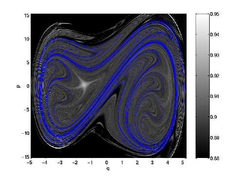
Figure 2: Phase space rendering of the Wigner function at time $t=149~{}\mbox{periods of driving}$. The early time part of the unstable manifold associated with the noise-free dynamics is shown in blue. The value of $D=10^{-3}$ is not sufficient to wipe out all the quantum interference which, as expected, is most prominent near turns in the manifold.

For more detailed evidence that, at $D=10^{-3}$, one is entering a semiclassical regime, in Fig. 2 we superimpose an image of the large scale features of the classical unstable manifold on top of the full quantum Wigner distribution at $D=10^{-3}$ after 149 drive periods [case (b) of Fig. 1]. The quantum phase space clearly exhibits local interference fringes around the large lobe-like structures associated with the short-time evolution of the unstable manifold. The appearance of local fringing about classical structures is direct evidence of a semiclassical evolution, where interference effects appear locally around the backbone of a classical evolution. This is in sharp contrast to the global diffraction pattern seen for $D=0$, where the contributions from individual curves cannot be distinguished, suppressing the appearance of any classical structure HabibDuff .

The arguments presented here do not apply directly to systems where the manifolds are non-compact (analogous to open flows in fluids). In this case noise does not necessarily lead to a termination of the structure production in phase space, hence a semiclassical approximation eventually fails. Thus the topological structure of the classical manifolds likely provides the physical underpinning of a proposed classification scheme for dynamical systems based on quantum-classical correspondence, originally stated in terms of spectral analysis of the density matrix 1 . An elaboration of both the mathematical analysis and numerical results will be presented in a companion paper Prep .

Numerical simulations were performed on the Cray T3E and IBM SP3 at NERSC, LBNL. B.D.G. and S.H. acknowledge support from the LDRD program at LANL. The work of B.S. and B.D.G (partially) was supported by the National Science Foundation grant #0099431. This research is supported by the Department of Energy, under contract W-7405-ENG-36.

References

- (1) M.V. Berry, in Les Houches Lecture Series LIV edited by M.-J. Giannoni, A. Voros, and J. Zinn-Justin (North-Holland, Amsterdam, 1991)
- (2) S. Habib, K. Jacobs, H. Mabuchi, R. Ryne, K. Shizume, and B. Sundaram, Phys. Rev. Lett. 88, 040402 (2002).
- (3) M.V. Berry and N.L. Balazs, J. Phys. A 12, 625 (1979).
- (4) G.P. Berman and G.M. Zaslavsky, Physica A 91, 450 (1978); G.P. Berman, A.M. Iomin and G.M. Zaslavsky, Physica D 4, 113 (1981).
- (5) C.M. Caves and G.J. Milburn, Phys. Rev. A 36, 5543 (1987).
- (6) H. Carmichael, An Open Systems Approach to Quantum Optics (Springer, Berlin, 1993).
- (7) T. Bhattacharya, S. Habib, and K. Jacobs, Phys. Rev. Lett. 85, 4852 (2000); Phys. Rev. A 67, 042103 (2003), and references therein.
- (8) K. Hepp, Helv. Phys. Acta 45, 237 (1972); W.H. Zurek, Phys. Rev. D 24, 1516 (1981); ibid 26, 1862 (1982); E. Joos and H.D. Zeh, Z. Phys. B 59, 223 (1985).
- (9) W.H. Zurek and J.P. Paz, Phys. Rev. Lett. 72, 2508 (1994).
- (10) A.R. Kolovsky, Phys. Rev. Lett. 76, 340 (1996).
- (11) G. Lindblad, Comm. Math. Phys. 48, 199 (1976); V. Gorini, A. Kossakowski, and E.C.G. Sudarshan, J. Math. Phys. 17 (1976) 821.
- (12) A.O. Caldeira and A.J. Leggett, Phys. Rev. A 31, 1059 (1985).
- (13) A.C. Doherty, K. Jacobs and G. Jungman, Phys. Rev. A 63, 062306 (2001).
- (14) E.P. Wigner, Phys. Rev. 40, 749 (1932).
- (15) S. Habib, K. Shizume, and W.H. Zurek, Phys. Rev. Lett. 80, 4361 (1998).
- (16) A.R.R. Carvalho, R.L. de Matos Filho, L. Davidovich, Phys. Rev. E 70, 026211 (2004).
- (17) C.W. Gardiner, Handbook of Stochastic Methods (Springer-Verlag, Berlin, 1996).
- (18) N.G. van Kampen, Stochastic Processes in Physics and Chemistry (North Holland, Amsterdam, 1992).
- (19) G.A. Voth, G. Haller and J.P. Gollub, Phys. Rev. Lett. 88, 254501 (2002).
- (20) See, e.g., M.V. Berry, Phil. Trans. Roy. Soc. A 287, 237 (1977); E.J. Heller, J. Chem. Phys. 67, 3339 (1977); S. Habib, Phys. Rev. D 42, 2566 (1990).
- (21) V.P. Maslov and M.V. Fedoriuk, Semi-Classical Approximation in Quantum Mechanics (Reidel, Holland, 1981).
- (22) E.J. Heller and S. Tomsovic, Phys. Today 7, 38 (1993); Phys. Rev. E 47, 282 (1993).
- (23) W.A. Lin and L.E. Ballentine, Phys. Rev. Lett. 65, 2927 (1990).
- (24) J. Guckenheimer and P. Holmes, Nonlinear Oscillations, Dynamical Systems, and Bifurcations of Vector Fields (Springer-Verlag, Berlin, 1986).
- (25) B.D. Greenbaum, S. Habib, K. Shizume, and B. Sundaram (in preparation).