Jump-like unravelings for non-Markovian open quantum systems

Abstract

Non-Markovian evolution of an open quantum system can be ‘unraveled’ into pure state trajectories generated by a non-Markovian stochastic (diffusive) Schrödinger equation, as introduced by Diósi, Gisin, and Strunz. Recently we have shown that such equations can be derived using the modal (hidden variable) interpretation of quantum mechanics. In this paper we generalize this theory to treat jump-like unravelings. To illustrate the jump-like behavior we consider a simple system: A classically driven (at Rabi frequency $\Omega$) two-level atom coupled linearly to a three mode optical bath, with a central frequency equal to the frequency of the atom, $\omega_{0}$, and the two side bands have frequencies $\omega_{0}\pm\Omega$. In the large $\Omega$ limit we observed that the jump-like behavior is similar to that observed in this system with a Markovian (broad band) bath. This is expected as in the Markovian limit the fluorescence spectrum for a strongly driven two level atom takes the form of a Mollow triplet. However the length of time for which the Markovian-like behaviour persists depends upon which jump-like unraveling is used.

I Introduction

In the past few years non-Markovian stochastic Schrödinger equations (SSEs) for diffusive unravelings have received considerable attention DioStr97 ; DioGisStr98 ; StrDioGis99 ; YuDioGisStr99 ; Cre00 ; Bud00 ; BasGhi02 ; GamWis002 ; GamWis003 ; Bas03 ; GamWis005 ; GamWis006 . A diffusive non-Markovian stochastic Schrödinger equation is a non-linear, non-Markovian, and stochastic evolution equation for a quantum state. We usually denote this quantum state by $|{\psi_{\{z_{k}(t)\}}(t)}\rangle$ where the subscripts $\{z_{k}(t)\}$ implies that $|{\psi_{\{z_{k}(t)\}}(t)}\rangle$ is conditioned on the set of continuous time dependent random variables $\{z_{k}(t)\}$ described by a probability distribution $P(\{z_{k}\},t)$. This set is constrained such that

$$\rho_{\rm red}(t)=E[|{\psi_{\{z_{k}(t)\}}(t)}\rangle\langle{\psi_{\{z_{k}(t)\}}(t)}|],$$ (1)

where $E[...]$ denotes an ensemble average over the set $\{z_{k}(t)\}$. Here $\rho_{\rm red}(t)$ refers to the reduced state of an open quantum system. An open quantum system is a combined system consisting of a “system of interest” and an environment or bath. The reduced state is defined by

$$\rho_{\rm red}(t)={\rm Tr}_{\rm env}[|{\Psi(t)}\rangle\langle{\Psi(t)}|].$$ (2)

Here $|{\Psi(t)}\rangle$ is the solution of the Schrödinger equation for the combined system (generally an entangled state) and ${\rm Tr}_{\rm env}[...]$ refers to a partial trace performed over the environments degrees of freedom.

In this paper we extend the known unravelings for non-Markovian SSEs to include two jump-like unravelings. This is motivated by the fact that in the Markovian limit the simplest of all Markovian SSEs is jump-like in nature. This corresponding to the direct detection quantum trajectory Car93 . However, as shown in Ref. GamWis002 in the non-Markovian case SSEs are not quantum trajectories. That is, they are not evolution equations for the state of the system conditioned on the outcomes of some continuous-in-time measurements of the bath. This is because a non-Markovian system remembers what has happen in the past (whether a measurement has occurred or not) and a continuously measured system will have a drastically different average evolution, $\rho(t)$, from a non-measured system $\rho_{\rm red}(t)$.

So what is the interpretation of non-Markovian SSEs? In Ref. GamWis005 we came to the conclusion that the three current non-Markovian SSEs, the coherent DioGisStr98 ; Cre00 ; GamWis002 , quadrature BasGhi02 ; GamWis002 and the position GamWis006 only have a non-trivial (non-numerical) interpretation when we consider the modal Fra81 ; Hea89 ; Die97 ; Bub97 ; BacDic99 ; Sud00 ; SpeSip01b ; GamWis004 (or Bell’s beable Bel84 ) interpretation of quantum mechanics. They are evolution equations for the system part of the property state of the universe when certain bath observables are given an objective reality (become hidden variables). The values of these bath hidden variables, at time $t$, are given by the set $\{z_{k}(t)\}$. The different unravelings correspond to a different choice of which bath observables are to be objective real. For example the position unraveling arises when the hidden variables for the bath correspond to the positions of each oscillator making up the bath GamWis005 ; GamWis006 . That is, the set $\{z_{k}(t)\}$ becomes the set $\{x_{k}(t)\}$ corresponding to the values of the positions of each oscillator of the bath. For this case the position trajectories, $\{d_{t}x_{k}(t)\}$, actually correspond to Bohmian trajectories Boh52a .

Note this is not the only interpretation of non-Markovian SSEs; in Refs. BasGhi02 and BasGhi03 Bassi and Ghirardi interpreted these equations as a new dynamical reduction modal, dynamical reduction with non-white Gaussian noise. In this paper we are not going to argue against this interpretation except to say that by accepting the above modal interpretation we can easily generalize the theory for diffusive non-Markovian SSEs to include jump-like “unravelings.”

A difference from the diffusive case is that it does not appear possible to derive an explicit expression for the jump-like non-Markovian SSEs. This is because these non-Markovian SSEs are conditioned on a discrete set $\{z_{n_{k}}(t)\}$ and as such it is impossible to define derivatives with respect to this set. Furthermore a Girsanov transformation DioGisStr98 can not be defined. In fact it turns out that to derive numerical jump-like non-Markovian unravelings is effectively the same as solving the Schrödinger equation for the combined system. Thus any numerical advantage of using non-Markovian SSE to determine $\rho_{\rm red}(t)$ [see Eq. (1)] is lost for these unravelings. However, the point of this paper is not to derive more effective ways of finding $\rho_{\rm red}(t)$ but rather to illustrate that by using the modal interpretation we can derive the numerical equivalent of the solution to a non-Markovian SSE for jump-like unravelings.

To illustrate a non-Markovian unraveling that exhibit jump-like behavior we consider the two unravelings, spectral-mode and temporal-mode. We apply our theory to a simple system: A classically driven two level atom (TLA), at Rabi frequency $\Omega$, coupled linearly to a three-mode optical bath, with a central frequency equal to the frequency of the atom, $\omega_{0}$, and the two side bands have frequencies $\omega_{0}\pm\Omega$. In the large $\Omega$ limit we observed that the jump-like behavior is similar to that observed in Markovian systems. This is expected as in the Markovian limit a strongly driven TLA has a fluorescent spectrum which takes the form of a Mollow triplet Mol75 with peaks at these frequencies.

The structure of this paper is as follows: In the next section we present an outline of the general physical model to which the theory of non-Markovian SSE is applicable. In Sec. III we present a review of the modal interpretation of quantum mechanics and how it applies to non-Markovian SSEs. In Secs. IV and V we derive two jump-like unravelings, these being the spectral-mode and the temporal-mode unraveling. In Sec VI we briefly outline how Jack, Collet and Walls JacColWal99 ; JacColWal99b ; JacCol00 non-Markovian quantum trajectory theory differs to our theory. Note other jump-like non-Markovian unravelings exists BreKapPet99 ; Bre03 , but these are only numerical methods for solving $\rho_{\rm red}(t)$, and as such will not be considered in this paper. Finally in Sec. VII we conclude this paper.

II The TLA and the underlying bath dynamics

The aim of this section is to outline the underlying model we will be using to generate jump-like non-Markovian unravelings. The standard model is to assume a preferred factorization of the universe into a system and environment, label by the Hilbert spaces ${\cal H}_{\rm sys}$ and ${\cal H}_{\rm env}$ respectively. The total Hamiltonian for the universe is then given by

$$\hat{H}_{\rm sys}(t)\otimes\hat{1}+\hat{1}\otimes\hat{H}_{\rm env}+\hat{V}.$$ (3)

Here $\hat{H}_{\rm sys}$, $\hat{H}_{\rm env}$ and $\hat{V}$ represent the Hamiltonians for the system, environment and any interaction taking place between the system and environment respectively. In this paper we assume the system is a two level atom (TLA) described by the free system Hamiltonian

$$\hat{H}_{\rm sys}(t)=\hat{H}_{\rm sys_{0}}+\hat{H}(t)=\frac{\hbar\omega_{0}}{2}\hat{\sigma}_{z}+\hat{H}(t),$$ (4)

where $\omega_{0}$ is the atomic transition frequency and $\hat{\sigma}_{z}$ is the Pauli spin operator

$$\hat{\sigma}_{z}=|{e}\rangle\langle{e}|-|{b}\rangle\langle{b}|,$$ (5)

where $|{e}\rangle$ and $|{b}\rangle$ represent the excited and ground state of the atom. The extra term $\hat{H}(t)$ in Eq. (4) represents any extra system evolution, for example a classical driving process.

The environment, as in all optical situations, is modelled by a collection of one-dimensional harmonic oscillators. The free Hamiltonian for this type of environment is

$$\hat{H}_{\rm env}=\sum_{k}^{\kappa}{\hbar\omega_{k}}\hat{a}^{\dagger}_{k}\hat{a}_{k},$$ (6)

where $\kappa$ defines the total number of modes, while $\omega_{k}$ and $\hat{a}_{k}$ ($\hat{a}_{k}^{\dagger}$) are the frequency and the annihilation (creation) operator of the $k^{\rm th}$ mode of the environment.

We assume that the interaction between the system and environment is consistent with the rotating wave approximation. That is, we assume $\hat{V}$ is linear in the environment amplitudes, and has the form

$$\hat{V}=i\hbar\sum_{k}^{\kappa}(g_{k}^{*}\hat{\sigma}\hat{a}_{k}^{\dagger}-g_{k}\hat{\sigma}^{\dagger}\hat{a}_{k}),$$ (7)

where $g_{k}$ is the coupling strength of the $k^{\rm th}$ mode to the system.

For calculational purposes we define an interaction frame such that the Hamiltonians $\hat{H}_{\rm sys_{0}}$ [which is defined implicity in Eq. (4)] and $\hat{H}_{\rm env}$ is removed. The unitary evolution operator for this transformations is

$$\hat{U}_{0}(t,0)=e^{-i(\hat{H}_{\rm sys_{0}}\otimes\hat{1}+\hat{1}\otimes\hat{H}_{\rm env})(t-0)/{\hbar}}.$$ (8)

Thus the combined state in the interaction frame is defined as

$$|{\Psi(t)}\rangle=\hat{U}_{0}^{\dagger}(t,0)|{\Psi(t)_{\rm Sch}}\rangle,$$ (9)

and an arbitrary operator $\hat{A}$ becomes

$$\hat{A}_{\rm int}(t)=\hat{U}_{0}^{\dagger}(t,0)\hat{A}\hat{U}_{0}(t,0).$$ (10)

This allows us to write the Schrödinger equation as

$$d_{t}|{{\Psi}(t)}\rangle=-\frac{i}{\hbar}[\hat{H}_{\rm int}(t)+\hat{V}_{\rm int}(t)]|{\Psi(t)}\rangle,$$ (11)

where $\hat{H}_{\rm int}(t)$ refers to $\hat{H}(t)$ in the interaction frame and $\hat{V}_{\rm int}(t)$ is defined as

$$\hat{V}_{\rm int}(t)=i\hbar\sum_{k}^{\kappa}[\hat{\sigma}g^{*}_{k}e^{i\Omega_{k}t}\hat{a}_{k}^{\dagger}-\hat{\sigma}^{\dagger}g_{k}e^{-i\Omega_{k}t}\hat{a}_{k}],$$ (12)

where $\Omega_{k}=\omega_{k}-\omega_{0}$.

In all the examples we present in this paper we take the extra system Hamiltonian, $\hat{H}(t)$, to be classical driving of the TLA. Under the dipole and rotating wave approximation the extra system Hamiltonian in Eq. (4) is

$$\hat{H}(t)=\frac{\hbar\Omega}{2}[\hat{\sigma}^{\dagger}\exp(-i\omega_{\rm c}t)+\hat{\sigma}\exp(i\omega_{\rm c}t)],$$ (13)

where $\Omega=-2{\bf d}\cdot{\bf E}_{0}({\bf r}_{0})/\hbar$ is the Rabi frequency and ${\bf E}_{0}({\bf r}_{0})$ is the amplitude of the classical field at the positions of the atom and ${\bf d}$ is dipole transition matrix. For simplicity we tune the frequency of the classical driving field, $\omega_{\rm c}$, to the atomic transition frequency. Thus when moving to the interaction frame Eq. (13) becomes

$$\hat{H}_{\rm int}=\frac{\hbar\Omega}{2}(\hat{\sigma}^{\dagger}+\hat{\sigma})=\frac{\hbar\Omega}{2}\hat{\sigma}_{x},$$ (14)

which is time independent.

III Modal interpretation of quantum mechanics

III.1 General modal dynamics

In this section we give a brief overview of the modal interpretation of quantum mechanics; for a more detailed description see Refs. Bel84 ; Bub97 ; BacDic99 ; Sud00 ; SpeSip01b ; GamWis004 . The basic idea of this view of quantum mechanics is that certain observables have an objective reality independent of measurement. This is in contrast to the orthodox interpretation where reality is undefined prior to measurement and it is the act of observation that defines the reality of the observable.

In quantum mechanics it is convenient to define an observable as

$$Z=\{(z_{n},\hat{\pi}_{n})\},$$ (15)

where the set of values $\{z_{n}\}$ correspond to the possible values the observable can have and $\{\hat{\pi}_{n}\}$ is the projective measure for the observable. When these values correspond to numbers we can write an observable as an operator

$$\hat{Z}=\sum_{n}z_{n}\hat{\pi}_{n}.$$ (16)

The projectors are orthogonal and form a decomposition of unity:

$$\sum_{n}\hat{\pi}_{n}=\hat{1}.$$ (17)

In quantum mechanics because of the non-commutative nature of observables, not all observables can be written in terms of the same projective measure $\{\hat{\pi}_{n}\}$. In the modal theory one postulates that only one set of projectors has an objective reality, this being called the preferred projective measure. Once this measure is specified it uniquely defines a group of observables which are objectively real, this being the group defined to have elements given by Eq. (15). In this paper we will refer to this group as the properties of the system. That is, the group of preferred observables (observables with objective reality) are labelled properties of the system.

The biggest criticism against the modal theory is that many choices of the preferred measure are viable Bub97 . This has lead to many variants of the modal interpretation of quantum mechanics Bel84 ; Bub97 ; BacDic99 ; Sud00 ; GamWis004 ; Boh52a ; Hea89 ; Die97 ; SpeSip01b . Some have tried to address the problem of choice, either by accepting it (the beable variant) Bel84 ; Bub97 ; Sud00 , selecting the position projective measure as preferred (Bohmian mechanics Boh52a ), or by applying an algorithm for determining the preferred projective measure based on the total wavefunction of the universe Bub97 ; BacDic99 ; Hea89 ; Die97 ; SpeSip01b . The algorithmic approaches in our opinion still face choice as one has to choose the preferred factorization of the universe. Furthermore we have shown in Ref. GamWis004 that we can extend the modal theory to include positive operator measures, thereby increasing the amount of possible choices. Here, however, we will only consider preferred projective measures and take the view that choice is fundamental. Depending on the physical situation we wish to describe we will choose the appropriate measure $\{\hat{\pi}_{n}\}$.

Once we have chosen the preferred projective measure, to explain why property $Z$ has the value $z_{n}$ at time $t$ we can introduce an extra quantum state, the property state. It is defined as

$$|{\Psi_{z_{n}(t)}(t)}\rangle=\hat{\pi}_{n}|{\Psi(t)}\rangle/\sqrt{N},$$ (18)

where $N$ is a normalization constant and $z_{n}(t)$ is the value of $Z$ at time $t$. The property state at time $t$ is determined by both $|{\Psi(t)}\rangle$ and a stochastic evolution (jumps between different $n$) . It is interpreted as the actual state of the universe, and by the eigenstate-eigenvalue link it selects the present value $z_{n}$ for property $Z$ from the possible values $\{z_{n}\}$. The stochastic dynamics (rates at which it jumps between different $n$) is determined by $|{\Psi(t)}\rangle$ and as such $|{\Psi(t)}\rangle$ in this interpretation is called the guiding state.

The modal dynamics (the stochastic evolution of the property state) is found using the method originally proposed by Bell Bel84 and generalized in Refs. BacDic99 ; Sud00 ; GamWis004 . We start by defining ${\rm Pr}(z_{n},t)$ as the probability that the property will have the value $z_{n}$ at time $t$. Assuming a Markovian process, by which we mean that the probability of the property being $z_{m}$ at time $t+dt$ only depends on the value at time $t$, we can write a master equation for ${\rm Pr}(z_{n},t)$ as

$$d_{t}{\rm Pr}(z_{n},t)=\sum_{m}[T_{nm}(t){\rm Pr}(z_{m},t)-T_{mn}{\rm Pr}(z_{n},t)],$$ (19)

where $T_{nm}$ (for $n\neq m$) are transition rates. For $n=m$, $T_{nn}$ (which is negative) is a measure of the rate at which value $z_{n}$ loses probability.

Defining a probability current $J_{nm}(t)$ as

$$J_{nm}(t)=T_{nm}(t){\rm Pr}(z_{m},t)-T_{mn}{\rm Pr}(z_{n},t),$$ (20)

results in $J_{nm}(t)=-J_{mn}(t)$ and allows us to rewrite the probability master equation as

$$d_{t}{\rm Pr}(z_{n},t)=\sum_{m}J_{nm}(t).$$ (21)

Given $J_{nm}(t)$ and ${\rm Pr}(z_{n},t)$, there are many possible transition rates satisfying Eq. (21). One solution, chosen by Bell Bel84 is as follows.

For $J_{nm}(t)<0$,

$$T_{nm}(t) = 0,$$ (22)

$$T_{mn}(t) = -J_{nm}(t)/{\rm Pr}(z_{n},t),$$ (23)

and for $J_{nm}(t)>0$

$$T_{nm}(t) = J_{nm}(t)/{\rm Pr}(z_{m},t),$$ (24)

$$T_{mn}(t) = 0.$$ (25)

Thus once we have the probability current it is possible to calculate the transition matrix $T_{nm}(t)$ which in turn allows us to calculate (via using a random number generator) a trajectory for the value of the property $Z$.

To find $J_{nm}(t)$, as in the orthodox theory, we have to postulate a fundamental rule for probability, the Born rule

$${\rm Pr}(z_{n},t)=\langle{\Psi(t)}|\hat{\pi}_{n}|{\Psi(t)}\rangle.$$ (26)

With this equation and Eqs. (21) and (11) a possible solution for $J_{nm}(t)$ is

$$J_{nm}(t) = 2{\rm Im}\{\langle{\Psi(t)}|\hat{\pi}_{n}[\hat{H}_{\rm int}(t)+\hat{V}_{\rm int}(t)]$$ (27)

$$\times\hat{\pi}_{m}|{\Psi(t)}\rangle\}{/\hbar}.$$

Note the ensemble set of trajectories we obtained for the value of the property $Z$ is only one of the infinitely many possible sets of ensemble trajectories. Others can be found by either adding an extra term $T^{0}_{nm}(t)$ to $T_{nm}(t)$, where $T^{0}_{nm}(t)$ is constrained only by

$$T_{nm}^{0}(t)P_{m}(t)-T_{mn}^{0}(t)P_{n}(t)=0,$$ (28)

or by adding any current $J_{nm}^{~{}0}(t)$ to $J_{nm}(t)$ which satisfies

$$\sum_{m}J_{nm}^{~{}0}=0.$$ (29)

For the purposes of this paper we only consider Bell solution [not containing the extra $T_{nm}^{0}(t)$ and $J_{nm}^{~{}0}(t)$ terms]. For a discussion of these solutions see Refs. Vin93 or Dic97 .

III.2 Application to non-Markovian SSEs

In Ref. GamWis005 we showed that the theory of the non-Markovian SSEs emerge from modal dynamics when we assume a preferred projective measure of the form

$$\{\hat{\pi}_{n}=\hat{1}_{\rm sys}\otimes\hat{\pi}_{n_{\rm env}}\},$$ (30)

where $\hat{\pi}_{n_{\rm env}}$ is a projector define solely to operate in the Hilbert space of the environment. (Note the coherent non-Markovian SSE DioStr97 ; DioGisStr98 ; StrDioGis99 ; YuDioGisStr99 ; Cre00 ; GamWis002 ; GamWis005 arises when we use a preferred POM rather than a projective measure; see Ref. GamWis005 ). This means the observables which have definite values are of the form

$$Z=\{z_{n},\hat{1}_{\rm sys}\otimes\hat{\pi}_{n_{\rm env}}\}.$$ (31)

That is, the bath is given property status, while the system is treated as a purely quantum system, which nevertheless influences the bath values via the coupling Hamiltonian [Eq. (12)].

Diffusive non-Markovian arise when the projective measure for the environment $\{\hat{\pi}_{n_{\rm env}}\}$ is chosen to be an infinitesimal projective density measure $\{\hat{\pi}(z)_{\rm env}dz\}$. That is, properties are given by

$$Z=\{z,\hat{1}_{\rm sys}\otimes\hat{\pi}(z)_{\rm env}dz\},$$ (32)

where $Z$ now has a continuous set of possible values $\{z\}$. For example the position unraveling occurs when we choose the following infinitesimal projective density measure

$$\{\hat{\pi}(x_{1})dx_{1}\otimes...\otimes\hat{\pi}(x_{k})dx_{k}\otimes...\otimes\hat{\pi}(x_{\kappa})dx_{\kappa}\},$$ (33)

where $\hat{\pi}(x_{k})=|{x_{k}}\rangle\langle{x_{k}}|$ and $|{x_{k}}\rangle$ is defined to be the eigenstate of the operator $\hat{x}_{k}=(\hat{a}_{k}+\hat{a}_{k}^{\dagger})/\sqrt{2}\,$. That is, the observables correspond to the positions of the environment’s $\kappa$ harmonic oscillators (and any function of them by the principle of property compositions BacDic99 ) are given property status. With this choice of preferred projective measure the property state of the universe becomes

$$|{\Psi_{\{x_{k}(t)\}}(t)}\rangle=|{\{x_{k}(t)\}}\rangle\otimes|{\psi_{\{x_{k}(t)\}}(t)}\rangle,$$ (34)

where $|{\psi_{\{x_{k}\}}(t)}\rangle$ is called the conditional system state. Here we see that the property state is divided into two parts, an environment state and system state.

In Ref. GamWis005 we showed that when using Bell’s solution for the transition parameters we can derive a set of $\kappa$ trajectories for the values of the $\kappa$ position properties, which we denote as $\{x_{k}(t)\}$ (these actually turn out to be Bohmian trajectories). Using these trajectories we can derive a differential equation for $|{\psi_{\{x_{k}(t)\}}(t)}\rangle$, which describes the evolution of the system part of the property state of the universe, the environment part is given by $|{\{x_{k}(t)\}}\rangle$. This system-state differential equation turns out to be the non-Markovian SSE for the position unraveling. For the complete derivation of this non-Markovian SSE and the other two diffusive non-Markovian SSEs see Refs. DioGisStr98 ; GamWis002 ; GamWis005 ; GamWis006 .

Here we are going to use the above reasoning to motivate how one can go about finding numerically the equivalent to the conditioned system state for jump-like unravelings. To do this we simply choose discrete rank one projectors for the environment. That is, the preferred projective measure is

$$\{\hat{\pi}_{n}\}=\{\hat{1}_{\rm sys}\otimes|{\{z_{n_{k}}\}}\rangle\langle{\{z_{n_{k}}\}}|\},$$ (35)

where $|{\{z_{n_{k}}\}}\rangle=|{z_{n_{1}}}\rangle\otimes...\otimes|{z_{n_{k}}}\rangle\otimes...\otimes|{z_{n_{\kappa}}}\rangle$ and $n=\{n_{1},n_{2},...,n_{\kappa}\}$. With this preferred projective measure the property state of the universe [see Eq. (18)] becomes

$$|{\Psi_{\{z_{n_{k}}(t)\}}(t)}\rangle=|{\{z_{n_{k}}(t)\}}\rangle\otimes|{\psi_{\{z_{n_{k}}(t)\}}(t)}\rangle,$$ (36)

where the conditioned state is

$$|{\psi_{\{z_{n_{k}}(t)\}}(t)}\rangle=\langle\{z_{n_{k}}(t)\}|{\Psi(t)}\rangle/\sqrt{N}.$$ (37)

The evolution of this state through time is equivalent to a non-Markovian SSE for jump-like unravelings.

To summarize, the procedure to developed numerical trajectories for both $|{\psi_{\{z_{n_{k}}(t)\}}(t)}\rangle$ and $\{z_{n_{k}}(t)\}$ is to first calculate the guiding state from the Schrödinger equation [see Eq. (11)], then using Bells solution we can determine both $J_{nm}(t)$ and $T_{nm}(t)$ for the appropriately chosen preferred projective measure. Once these are calculated we use a random number generator to simulate simultaneously a typical trajectory for $\{z_{n_{k}}(t)\}$ and hence $|{\psi_{\{z_{n_{k}}(t)\}}(t)}\rangle$.

IV The spectral mode unraveling

The first unraveling we consider is the simplest of all; it corresponds to the bath hidden variables being the photon number of each bath spectral mode. That is, the values of the bath hidden variables are denoted by $\{n_{k}\}$ and only take on discrete values. The preferred projective measure for this unraveling is

$$\{\hat{\pi}_{n}\}=\{\hat{1}_{\rm sys}\otimes|{\{{n_{k}}\}}\rangle\langle{\{{n_{k}}\}}|\},$$ (38)

where $|{\{{n_{k}}\}}\rangle=|{{n_{1}}}\rangle\otimes...\otimes|{{n_{k}}}\rangle\otimes...\otimes|{{n_{\kappa}}}\rangle$ and $|{{n_{k}}}\rangle$ is the eigenstate of the spectral number operator $\hat{n}_{k}=\hat{a}_{k}^{\dagger}\hat{a}_{k}$.

To illustrate this unraveling we consider two cases of a driven TLA coupled to the bath. In the first the ‘bath’ is a single mode harmonic oscillator and in the second the bath consists of three modes as described in the introduction.

IV.1 A single-mode bath

The first example consists of a bath with only one mode ($\kappa=1$). Thus it only has one bath hidden variable with value $n$ at time $t$. Thus $n(t)$ denotes the trajectory of this value through time. By Eq. (12) the interaction Hamiltonian in the interaction frame with the free dynamics removed is

$$\hat{V}_{\rm int}(t)=i\hbar[g^{*}e^{i(\omega_{1}-\omega_{0})t}\hat{\sigma}\hat{a}^{\dagger}-ge^{-i(\omega_{1}-\omega_{0})t}\hat{\sigma}^{\dagger}\hat{a}].$$ (39)

Choosing the bath frequency, $\omega_{1}=\omega_{0}$ and including the driving of the TLA the evolution for the guiding state is determined by

$$d_{t}|{{\Psi}(t)}\rangle=\Big{[}-\frac{i\Omega}{2}\hat{\sigma}_{x}+g^{*}\hat{\sigma}\hat{a}^{\dagger}-g\hat{\sigma}^{\dagger}\hat{a}\Big{]}|{\Psi(t)}\rangle.$$ (40)

To calculate the stochastic evolution of the property state, $|{\Psi_{n(t)}(t)}\rangle=|{n(t)}\rangle|{\psi_{n(t)}(t)}\rangle$, we use Bell’s solution to find $J_{nm}(t)$ [see Eq. (27)]. Doing this we get

$$J_{nm}(t)=2{\rm Im}\{\langle{\tilde{\psi}_{n}(t)}|\langle{n}|[ig^{*}\hat{\sigma}\hat{a}^{\dagger}-ig\hat{\sigma}^{\dagger}\hat{a}]|{m}\rangle|{\tilde{\psi}_{m}(t)}\rangle\}.$$ (41)

where $|{\tilde{\psi}_{n}(t)}\rangle=\langle{n}|{\Psi(t)}\rangle$ is the unnormalised conditioned state in configuration space. This simplifies to

$$J_{nm}(t) = -2{\rm Im}[ig\langle{\tilde{\psi}_{n}(t)}|\hat{\sigma}^{\dagger}|{\tilde{\psi}_{m}(t)}\rangle\sqrt{n+1}\,\delta_{n+1,m}]$$ (42)

$$+2{\rm Im}[ig^{*}\langle{\tilde{\psi}_{n}(t)}|\hat{\sigma}|{\tilde{\psi}_{m}(t)}\rangle\sqrt{n}\,\delta_{n-1,m}].{\hskip 19.91684pt}$$

Here we see that for a given $m$ only $J_{m\pm 1,m}(t)$ are non-zero. Thus the only transitions allowed are from $m\rightarrow m\pm 1$. The transition matrices [see Eqs. (22) - (25)] are as follows.

For $J_{m+1,m}(t)>0$ (or $J_{m-1,m}(t)<0$),

$$T_{m+1,m}(t) = J_{m+1,m}(t)/{\rm Pr}(z_{m},t)$$ (43)

$$= 2{\rm Im}\Big{[}ig^{*}\langle{{\psi}_{m+1}(t)}|\hat{\sigma}|{{\psi}_{m}(t)}\rangle$$

$$\times\sqrt{\frac{({m+1}){\rm Pr}({m+1},t)}{{\rm Pr}(m,t)}}\,\Big{]},$$

$$T_{m-1,m}(t) = 0,$$ (44)

and for $J_{m+1,m}(t)<0$ (or $J_{m-1,m}(t)>0$),

$$T_{m+1,m}(t) = 0,$$ (45)

$$T_{m-1,m}(t) = J_{m-1,m}(t)/{\rm Pr}(z_{m},t)$$ (46)

$$= -2{\rm Im}\Big{[}ig\langle{{\psi}_{m-1}(t)}|\hat{\sigma}^{\dagger}|{{\psi}_{m}(t)}\rangle$$

$$\times\sqrt{\frac{m{\rm Pr}({m-1},t)}{{\rm Pr}(m,t)}}\,\Big{]}.$$

Using a random number generator we can simulate a typical trajectory for $n(t)$ based on the above transition rates. For example given that $n(t)$ is $m$ at time $t$, depending on which one of $J_{m\pm 1,m}(t)$ is positive [$J_{m+1,m}(t)$ or $J_{m-1,m}(t)$] determines whether the value of the bath hidden variable is going to jump up or down in the interval $dt$. Let us assume $J_{m+1,m}(t)$ is positive then the probability of an upward jump in the interval $dt$ is $T_{m+1,m}(t)dt$, the simulation works by choosing a random variable between $[0,1]$ and if $T_{m+1,m}(t)dt$ is greater than this an upward jump occurs. This procedure is then repeated until the desired simulation time is reached. Note in Eqs. (43) – (46) how the conditioned state in configuration space, $|{\psi_{n}(t)}\rangle$, guides $n(t)$. However, unlike diffusive non-Markovian we can see here, explicitly, that it is impossible to define this transition in terms of only one conditioned state, thus no analytical evolution equation for $|{\psi_{n(t)}(t)}\rangle$ can be derived.

Choosing $\Omega=5g$ a numerical simulation for a typical trajectory is shown in Fig. 1 in Bloch representation

$$x(t) = \langle\hat{\sigma}_{x}\rangle_{t},$$ (47)

$$y(t) = \langle\hat{\sigma}_{y}\rangle_{t},$$ (48)

$$z(t) = \langle\hat{\sigma}_{z}\rangle_{t},$$ (49)

where $\langle\hat{A}\rangle_{t}=\langle{\psi_{n(t)}(t)}|\hat{A}|{\psi_{n(t)}(t)}\rangle$. Also shown in this figure is the trajectory for the value of the hidden value, $n(t)$. Here it is observed that the conditioned state evolves smoothly until there is a jump in $n(t)$. Most of jumps are up in photon number (all except one which occurs at large $t$). This is because with classical driving we are effectively adding energy to the system and for it to dissipate this energy photons are emitted from the atom into the bath. This is further verified by the fact that for most jumps there is a corresponding lowering of atomic energy [that is, a lowering of $z(t)$]. Note for Markovian dynamics an upward jump in photon number always puts the system in the ground state ($z=-1$). However in this figure this is not observed and in fact (for large time in the figure) there are upward jumps in atomic energy when the value of $n(t)$ increases. This clearly shows that non-Markovian dynamics is a lot more complicated than Markovian. Note the above strange behaviour (not Markovian-like) becomes more evident at later times, when there are many photons in the bath. This is expected since in the Markovian case there is never more then one photon per bath mode on average.

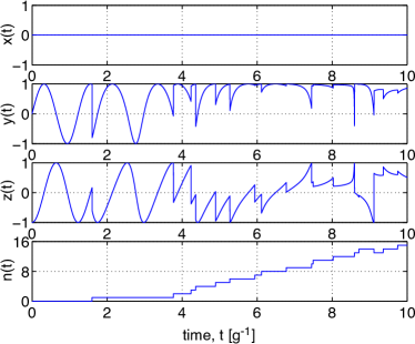
Figure 1: This figure depicts a typical trajectory in Bloch representation for the spectral mode unraveling when the system is a driven TLA and the bath is a single mode harmonic oscillator. In this figure all calculations were done using the initial system state $|{\psi(0)}\rangle=|{b}\rangle$ with system parameters $g=1$, $\Omega=5$. Time is measured in units $g^{-1}$.

To show that by performing an ensemble average over these trajectories do in fact give the reduced state, the difference between the ensemble average of 1000 trajectories and the actual reduced state is shown in Fig. 2. Here it is observed that to within statistical error these methods agree.

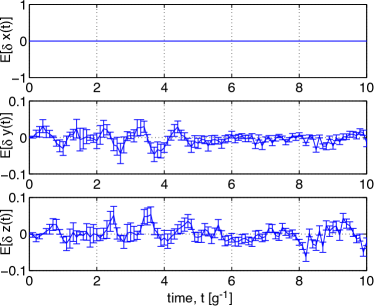
Figure 2: This figure depicts the difference between the ensemble average of 1000 trajectories and the actual reduced state for the spectral mode unraveling when the system is a driven TLA and the bath is a single mode harmonic oscillator. All parameters are defined in Fig. 1.

IV.2 The three mode bath

In the above example we observed that it is possible to derive numerically the equivalent to a non-Markovian SSE for the spectral mode unraveling for a simple system. Now we consider a slightly more complicated system: a TLA coupled linearly to a three mode optical bath, with a central frequency equal to the frequency of the atom, $\omega_{0}$, and the two side bands have frequencies $\omega_{0}\pm\Omega$. That is, the interaction Hamiltonian [Eq. (12)] becomes

$$\hat{V}_{\rm int}(t)=i\hbar\sum_{k=-1}^{1}[\hat{\sigma}g^{*}_{k}e^{ik\Omega t}\hat{a}_{k}^{\dagger}-\hat{\sigma}^{\dagger}g_{k}e^{-ik\Omega t}\hat{a}_{k}].$$ (50)

With this interaction Hamiltonian the guiding state evolution is determined by

$$d_{t}|{{\Psi}(t)}\rangle = \Big{\{}-\frac{i\Omega}{2}\hat{\sigma}_{x}+\sum_{k=-1}^{1}[\hat{\sigma}g^{*}_{k}e^{ik\Omega t}\hat{a}_{k}^{\dagger}-\hat{\sigma}^{\dagger}g_{k}$$ (51)

$$\times e^{-ik\Omega t}\hat{a}_{k}]\Big{\}}|{\Psi(t)}\rangle.$$

As in the last example, to calculate the stochastic evolution of the property state [$|{\Psi_{\{n_{k}(t)\}}(t)}\rangle=|{\{n_{k}(t)\}}\rangle|{\psi_{\{n_{k}\}}(t)}\rangle$], we use Bell’s solution to find $J_{n_{-1},m_{-1};n_{0},m_{0};n_{1},m_{1}}(t)$ [see Eq.(27)]. Here we find that only six values of $J_{n_{-1},m_{-1};n_{0},m_{0};n_{1},m_{1}}(t)$ are non-zero.

We expect that in the short time and large driving limit the conditioned state will jump between approximate $\hat{\sigma}_{x}$ eigenstates ($|{{\sigma}_{x}=1}\rangle$ and $|{{\sigma}_{x}=-1}\rangle$). This expectation can be illustrated analytically by considering the following argument. We move to a second interaction frame, this being the frame with both the free dynamics (standard interaction frame) and $H_{\rm int}$ removed. That is, the interaction Hamiltonian is

$$\hat{V}_{\rm int^{\prime}}(t) = i\hbar\sum_{k=-1}^{1}\Big{\{}g_{k}^{*}[\hat{\sigma}_{x}+\hat{\sigma}_{x}^{+}e^{i\Omega t}+\hat{\sigma}_{x}^{-}$$ (52)

$$\times e^{-i\Omega t}]\hat{a}_{k}^{\dagger}e^{ik\Omega t}-g_{k}[\hat{\sigma}_{x}+\hat{\sigma}_{x}^{+}e^{i\Omega t}$$

$$+\hat{\sigma}_{x}^{-}e^{-i\Omega t}]\hat{a}_{k}e^{-ik\Omega t}\Big{\}}/2,$$

where

$$\hat{\sigma}_{x}^{+} = |{{\sigma}_{x}=1}\rangle\langle{{\sigma}_{x}=-1}|,$$ (53)

$$\hat{\sigma}_{x}^{-} = |{{\sigma}_{x}=-1}\rangle\langle{{\sigma}_{x}=1}|,$$ (54)

and the prime denotes rotation to a second interaction frame.

We can now make the assumption that that for large driving all sinusoidally varying terms can be neglected (this is effectively a second RWA). Thus Eq. (52) becomes

$$\hat{V}_{\rm int^{\prime}}(t) = i\hbar\Big{\{}g_{-1}^{*}\hat{\sigma}_{x}^{+}\hat{a}_{-1}^{\dagger}-g_{-1}\hat{\sigma}_{x}^{-}\hat{a}_{-1}+g_{0}^{*}\hat{\sigma}_{x}\hat{a}_{0}^{\dagger}$$

$$-g_{0}\hat{\sigma}_{x}\hat{a}_{0}+g_{1}^{*}\hat{\sigma}_{x}^{-}\hat{a}_{1}^{\dagger}-g_{1}\hat{\sigma}_{x}^{+}\hat{a}_{1}\Big{\}}/2.$$

Moving back to the original interaction frame results in

$$\hat{V}_{\rm int}(t) = i\hbar\Big{\{}g_{-1}^{*}\hat{\sigma}_{x}^{+}\hat{a}_{-1}^{\dagger}e^{-i\Omega t}-g_{-1}\hat{\sigma}_{x}^{-}\hat{a}_{-1}e^{i\Omega t}+$$ (56)

$$g_{0}^{*}\hat{\sigma}_{x}\hat{a}_{0}^{\dagger}-g_{0}\hat{\sigma}_{x}\hat{a}_{0}+g_{1}^{*}\hat{\sigma}_{x}^{-}\hat{a}_{1}^{\dagger}e^{i\Omega t}$$

$$-g_{1}\hat{\sigma}_{x}^{+}\hat{a}_{1}e^{-i\Omega t}\Big{\}}/2.$$

That is, in the large driving limit Eq. (50) approximates to the above Hamiltonian. Now since $\hat{\sigma}_{x}^{-}$ and $\hat{\sigma}_{x}^{+}$ are lowering and raising operators for the $\hat{\sigma}_{x}$ basis we can conclude that when there is a transition from the $|{{\sigma}_{x}=1}\rangle$ to $|{{\sigma}_{x}=-1}\rangle$ eigenstates there is a corresponding upward jump in the photon number for the higher-frequency mode or a lowering in the photon number for the lower-frequency mode. The transition from the $|{{\sigma}_{x}=-1}\rangle$ to $|{{\sigma}_{x}=1}\rangle$ eigenstate result in jumps of opposite nature. A jump in the photon number for the central-mode should not change the conditioned state.

These predictions are verified in Figs. 3 (A) and (B) where we show simulations of the exact Bell dynamics with interaction Hamiltonian Eq. (50). Note the slight variation from the above prediction which we believe is due to the fact that the driving is not infinite. The first figure shows a typical trajectory for the conditioned state for parameters $g_{-1}=g_{0}=g_{1}=1$, and $\Omega=20g$ for the first 10 units of time whereas the second figure shows the next 10 units of time. It is in this second period of time where downward jumps in the outer modes are observed.

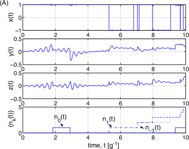
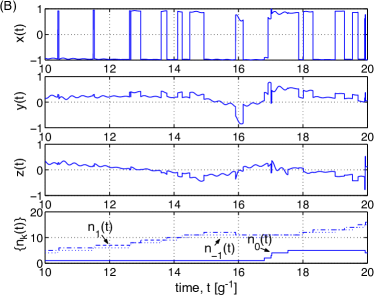
Figure 3: This figure depicts a typical trajectory in Bloch representation for the spectral-mode unraveling when the system is a driven TLA and the bath consists of 3 modes. In this figure all calculations were done using the initial system state $|{\psi(0)}\rangle=(|{e}\rangle+|{b}\rangle)/\sqrt{2}\,$ with parameters $g_{-1}=g_{0}=g_{1}=1$, and $\Omega=20g$. Time is measured in units $g^{-1}$. Part (A) is for $0\leq t<10$ and part (B) for $10\leq t<20$.

The prime motivation behind considering this 3-mode system is that in the strong driving limit the jump dynamics should exhibit similar features to those observed in a spectral-mode unraveling of a Markovian open quantum system. This is because in the large driving limit the fluorescence of a driving TLA takes the form of a Mollow spectrum Mol75 ; Lou83 [Fig. 4 shows this fluorescence spectrum (line graph) for $\Omega$ equal to $20$ times the spontaneous emission rate, $\gamma$]. In the large driving limit the Mollow spectrum approaches becoming delta functions centered on the frequencies $\omega_{0}-\Omega$, $\omega_{0}$, and $\omega_{0}+\Omega$. Thus one would expect that in this limit an unraveling in terms of spectral modes would have similar dynamics in both a non-Markovian and Markovian open quantum system. But what is the spectral-mode unraveling for a Markovian open quantum system. In Ref. WisToo99 an unraveling of a driven TLA with a Markovian system-bath interaction using filter cavities and photdetectors was introduced. We call this the Wiseman and Toombes filtered Markovian (WTFM) unraveling. (Note this unraveling is an example of an unraveling of a Markovian open quantum system which has non-Markovian conditioned state evolution for the atom). In this unraveling the field emitted by the atom is detected using two cavities tuned to the sidebands of the Mollow triplet (these act as mode filters). Thus in the strong driving limit the WTFM unraveling effectively corresponds to a spectral-three-mode unraveling. In Ref. WisToo99 it was observed that in this limit the conditioned state for the TLA jumps between almost $\hat{\sigma}_{x}$ eigenstates. Note, the non-Markovian case differs from the WTFM in that it is possible to get downward jumps in photon number. In the Markovian case this is not possible. However, as before, these anomalous events become more frequent as the modes become more populated.

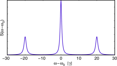
Figure 4: This figure depicts the fluorescence spectrum for a Markovian driven TLA with $\Omega$ equal to $20$ times the spontaneous emission rate, $\gamma$.

V Temporal-mode unraveling

In the Markovian limit the simplest Markovian SSE is direct detection. This detection scheme involves measurements performed into temporal modes of the system (rather than the frequency modes) Car93 . A temporal mode is best defined by considering the electromagnetic field operator $\hat{\bf E}({\bf r})$. The standard definition of this (neglecting polarization) is TitGla66

$$\hat{\bf E}({\bf r})=-i\sum_{k}^{\kappa}\hat{a}_{k}^{\dagger}{\bf u}^{*}_{k}({\bf r})+i\sum_{k}^{\kappa}\hat{a}_{k}{\bf u}_{k}({\bf r})$$ (57)

where ${\bf u}_{k}({\bf r})$ if the mode function for the $k^{\rm th}$ frequency (spectral) mode. This can be rewritten as

$$\hat{\bf E}({\bf r})=-i\sum_{\tau}^{\kappa}\hat{b}_{\tau}^{\dagger}{\bf v}^{*}_{\tau}({\bf r})+i\sum_{\tau}^{\kappa}\hat{b}_{\tau}{\bf v}_{\tau}({\bf r}),$$ (58)

where ${\bf v}_{\tau}({\bf r})$ labels a new type of mode with annihilation and creation operators $\hat{b}_{\tau}$ and $\hat{b}_{\tau}^{\dagger}$. These new modes can be related to the frequency modes by

$$\hat{b}_{\tau}=\sum_{k}^{\kappa}\hat{a}_{k}\gamma_{\tau,k}^{*},$$ (59)

where $\gamma_{\tau,k}$ are the elements of a unitary matrix ($\sum_{\tau}\gamma_{\tau,k}^{*}\gamma_{\tau,k^{\prime}}=\delta_{k,k^{\prime}}$ ). Choosing $\gamma_{\tau,k}$ to give a discrete fourier transform,

$$\hat{b}_{\tau} = \frac{1}{\sqrt{\kappa}\,}\sum_{k}^{\kappa}\hat{a}_{k}\exp(-i2\pi\tau k/\kappa),$$ (60)

$$\hat{a}_{k} = \frac{1}{\sqrt{\kappa}\,}\sum_{\tau}^{\kappa}\hat{b}_{\tau}\exp(i2\pi\tau k/\kappa),$$ (61)

results in ${\bf v}_{\tau}({\bf r})$ having the functional form of a temporal mode.

Since we have now defined an annihilation operator for the temporal mode it is possible to define the observable to which we wish to give an objective reality. This is the temporal-mode-number operator, $\hat{I}_{\tau}=\hat{b}_{\tau}^{\dagger}\hat{b}_{\tau}$. Thus the preferred projective measure for this unraveling is

$$\{\hat{\pi}_{n}\}=\{\hat{1}_{\rm sys}\otimes|{\{{I_{n_{\tau}}}\}}\rangle\langle{\{{I_{n_{\tau}}}\}}|\},$$ (62)

where $|{\{{I_{n_{\tau}}}\}}\rangle=|{I_{n_{1}}}\rangle\otimes...\otimes|{I_{n_{\tau}}}\rangle\otimes...\otimes|{I_{n_{\kappa}}}\rangle$, and $|{I_{n_{\tau}}}\rangle$ is an eigenstate of $\hat{I}_{\tau}$. This set of operators $\{\hat{I}_{\tau}\}$ are the hidden variables for this unraveling. Each operator $\hat{I}_{\tau}$ takes one of its possible integer values $\{{I}_{n_{\tau}}\}$.

To provide a clearer picture of this unraveling we consider briefly the Markovian case. In the Markovian limit the number of modes becomes continuous ($\kappa\rightarrow\infty$) and the system-bath coupling becomes flat ($g_{k}\rightarrow\sqrt{\gamma/2}\,$). As such we must define continuous (in frequency) annihilation operators $\hat{a}(\tilde{\omega})$ where $\tilde{\omega}=\omega-\omega_{0}$ with $\omega$ being a continues variable labelling the frequency of the bath. This results in the temporal modes, denoted by $\hat{b}(\tau)$, becoming continuous in time and being related to $\hat{a}(\tilde{\omega})$ by the fourier transform

$$\hat{b}(\tau) = \frac{1}{\sqrt{2\pi}\,}\int_{-\infty}^{\infty}\hat{a}(\tilde{\omega})\exp(-i\tilde{\omega}\tau)d\tilde{\omega}.,$$ (63)

$$\hat{a}(\tilde{\omega}) = \frac{1}{\sqrt{2\pi}\,}\int_{-\infty}^{\infty}\hat{b}(\tau)\exp(i\tilde{\omega}\tau)d\tau$$ (64)

Furthermore the interaction Hamiltonian, Eq. (12) (this is in the interaction frame with the free system and bath dynamics removed) becomes

$$\hat{V}_{\rm int}(t)=i\hbar\sqrt{\frac{\gamma}{2\pi}}\,\int_{-\omega_{0}}^{\infty}[\hat{\sigma}e^{i\tilde{\omega}t}\hat{a}^{\dagger}(\tilde{\omega})-\hat{\sigma}^{\dagger}e^{-i\tilde{\omega}t}\hat{a}(\tilde{\omega})]d\tilde{\omega}.$$ (65)

Assuming that $\omega_{0}$ is large (this is valid for optical situations), with little error the lower limits of the integrals can be taken as $\infty$ GarZol00 . This then allows us to rewrite Eq. (65) as

$$\hat{V}_{\rm int}(t)=i\hbar\sqrt{{\gamma}}\,\int_{-\infty}^{\infty}[\hat{\sigma}\delta(\tau-t)\hat{b}^{\dagger}(\tau)-\hat{\sigma}^{\dagger}\delta(t-\tau)\hat{b}(\tau)]d\tau.$$ (66)

Here we see that at time $t$ only one temporal mode is coupled to the system. This is precisely why the bath in a Markovian open quantum system only effects the system at one time (no memory effects).

For a non-Markovian open quantum system the above delta correlations will not exists and as such the bath will have a memory. Writing Eq. (12) in terms of the discrete temporal modes [Eq. (60)] gives

$$\hat{V}_{\rm int}(t) = i\hbar\sum_{\tau}^{\kappa}[c_{\tau}^{*}(t)\hat{\sigma}\hat{b}_{\tau}^{\dagger}-c_{\tau}(t)\hat{\sigma}^{\dagger}\hat{b}_{\tau}],$$ (67)

where

$$c_{\tau}(t) = \frac{1}{\sqrt{\kappa}\,}\sum_{k}^{\kappa}g_{k}e^{-i\Omega_{k}t+i2\pi\tau k/\kappa}.$$ (68)

This clearly does not have a delta correlation between $t$ and $\tau$ as occurs in the Markovian case [Eq. (66)]. To show that this does occur in the Markovian limit we simply let $g_{k}$ become flat ($g_{k}=g$) and assume a constant spacing in frequency $\Omega_{k}=k\Omega$. Doing this results in

$$c_{\tau}(t)=\frac{g}{\sqrt{\kappa}\,}\Big{\{}1+2\sum_{k=1}^{(\kappa-1)/2}\cos[k(\Omega t-2\pi\tau/\kappa)]\Big{\}}.$$ (69)

This by definition is a Kronecker $\delta$-function in the $\kappa\rightarrow\infty$ limit. This in turn implies a Dirac $\delta$-function in the continuous limit.

To illustrate this unraveling we consider a driven TLA coupled to a three mode bath as before. For the three mode case Eq. (60) becomes

$$\hat{b}_{\tau}=\frac{1}{\sqrt{3}\,}\sum_{k=-1}^{1}\hat{a}_{k}\exp(-i2\pi\tau k/3).$$ (70)

Using these operators we can rewrite the interaction Hamiltonian, Eq. (67), as

$$\hat{V}_{\rm int}(t) = i\hbar\sum_{\tau=-1}^{1}[c_{\tau}(t)\hat{\sigma}\hat{b}_{\tau}^{\dagger}-c_{\tau}(t)\hat{\sigma}^{\dagger}\hat{b}_{\tau}].$$ (71)

where

$$c_{\tau}(t)=\frac{g}{\sqrt{3}\,}\Big{\{}1+2\cos(\Omega t-2\pi\tau/3)\Big{\}}.$$ (72)

Here we have assumed $g_{-1}=g_{0}=g_{1}=g$ as before. Although these functions are not $\delta$-functions, $c_{\tau}^{2}(t)$ are peaked at times $t=2\pi(\tau/3+n)/\Omega$ for $n$ an integer, as shown in the finial plot of Fig. 5.

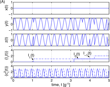
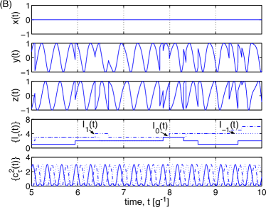
Figure 5: This figure depicts a typical trajectory in Bloch representation for the temporal-mode unraveling when the system is a driven TLA and the bath consists of 3 modes. In this figure all calculations were done using the initial system state $|{\psi(0)}\rangle=|{b}\rangle$ with parameters $g_{-1}=g_{0}=g_{1}=1$, and $\Omega=20g$. Time is measured in units $g^{-1}$. Part (A) is for $0\leq t<5$ and part (B) for $5\leq t<10$.

Using the same techniques as in the last unraveling it is possible to determined a probability current $J_{n_{1},m_{1};n_{2},m_{2};n_{3},m_{3}}(t)$. Then we can find a typical trajectory for the values of the bath hidden variables $\{I_{n_{\tau}}(t)\}$ and a numerical trajectory for the condition state $|{\psi_{\{I_{n_{\tau}}(t)\}}(t)}\rangle$. Figures 5 (A) and (B) illustrates a typical trajectory for a driven TLA with driving frequency $\Omega=20g$. Here we see that the dynamics are clearly unlike that observed for a Markovian open quantum system under a temporal-mode unraveling (direct detection). In the Markovian case an upward jump in the temporal mode corresponds to the conditioned system state jumping to the ground state ($z=-1$); see Ref. Car93 . However for an upward jump into the $\tau^{\rm th}$ temporal mode which occurs when $c_{\tau}^{2}(t)$ is a maximum this behaviour is observed, and the closer $c_{\tau}^{2}(t)$ is to maximum the closer the conditioned state jumps to $z=-1$. Thus we expect that when there are enough modes such that at every time $t$ one of the $c_{\tau}^{2}(t)^{\prime}s$ is a maximum (Markovian limit) an upward jump in photon number will result in the system state jumping to the ground state. Note, as in all the other examples at later times when the modes become populated extra non-Markovian features are present. Firstly downward jumps in temporal mode number are present. These result in the conditioned state jumping towards the excited state ($z=1$). But more interesting at approximately $t=4.9g^{-1}$ (as well as at $t=9.5g^{-1}$), there is a upward jump in the $\tau=-1$ ($\tau=0$) temporal mode which results in an increasing of atomic energy (the conditioned state jumping towards a higher atomic energy state).

VI Comparison with Jack, Collet, and Walls

Recently Jack, Collet and Walls (JCW) have published a series of papers, Refs. JacColWal99 ; JacColWal99b ; JacCol00 , where they developed a quantum trajectory theory (continuous in time measurement theory) for non-Markovian systems which incorporates jump-like unravelings. Thus the aim of this section is to review their theory and discuss how it differs from ours.

In the JCW theory, because it concerns measurements, they have to add the requirement, “a measurement at a certain time does not disturb any future measurements” JacCol00 . This basically means that the average state of the system (average over all possible measurements records) must be equal to the reduced state. Thus there is no back action on the system from the measurements. How is this possible? For argument’s sake, consider two consecutive quantum non-demolition measurements of the bath observable

$$Z=\{(z_{n},\hat{1}_{\rm sys}\otimes|{z_{n}}\rangle\langle{z_{n}}|)\}.$$ (73)

Then we can write the average state of the system as

$$\rho(t) = \sum_{n,m}\langle{z^{(2)}_{n}}|\hat{U}(t_{2},t_{1})|{z^{(1)}_{m}}\rangle\langle{z^{(1)}_{m}}|\hat{U}(t_{1},0)|{\Psi(0)}\rangle$$

$$\times\langle{\Psi(0)}|\hat{U}^{\dagger}(t_{1},0)|{z^{(1)}_{m}}\rangle\langle{z^{(1)}_{m}}|\hat{U}^{\dagger}(t_{2},t_{1})|{z^{(2)}_{n}}\rangle$$

where the superscripts $(1)$ and $(2)$ refer to the first measurement made at time $t_{1}$ and the second measurement made at time $t_{2}$. This is only equal to the reduced state, Eq. (2), if $[\hat{U}(t_{2},t_{1}),|{z^{(1)}_{m}}\rangle\langle{z^{(1)}_{m}}|]=0$. This implies that either $\hat{U}(t_{2},t_{1})$ is diagonal in the bath basis $\{|{z^{(1)}_{m}}\rangle\}$ or $\hat{U}(t_{2},t_{1})$ and $\{|{z^{(1)}_{m}}\rangle\langle{z^{(1)}_{m}}|\}$ operate on separate Hilbert spaces. This is precisely what happens in the Markovian limit (because of the delta correlations between the bath noise operators GarZol00 ). JCW theory uses the later case also and proposes that we can define a field quantity $\hat{\phi}(t)$ to be measured, such that

$$[\hat{\phi}(t),\hat{\phi}^{\dagger}(t^{\prime})]=\delta(t-t^{\prime}).$$ (75)

However, apart from Markovian open quantum systems it is not clear what measurement schemes this is applicable too. JCW consider in Ref. JacColWal99 a non-Markovian unraveling of a Markovian open quantum system, this being their spectral detection unraveling. This is similar to the WTFM unraveling, except they do not extend the system to include cavities.

In the JCW theory to account for the the memory effects of non-Markovian unravelings it is imposable to assign a pure state for the system at time $t$ conditioned on a past measurement record, ${\bf I}_{[0,t]}$ (a string of results $r_{1},...,r_{k}$ where $t=k\delta t$). Instead the state of the system conditioned on the measurement record ${\bf I}_{[0,t]}$ is given by

$$\rho_{{\bf I}_{[0,t]}}(t)=\frac{\tilde{\rho}_{{\bf I}_{[0,t]}}(t)}{{\rm Pr}({\bf I}_{[0,t]})},$$ (76)

where

$${\rm Pr}({\bf I}_{[0,t]})=\int d\{r_{\frac{s}{\delta t}>\frac{t}{\delta t}}\}\langle{\tilde{\psi}_{{\bf I}_{[0,s]}}(t)}|{\tilde{\psi}_{{\bf I}_{[0,s]}}(t)}\rangle$$ (77)

and

$$\tilde{\rho}_{{\bf I}_{[0,t]}}(t)=\int d\{r_{\frac{s}{\delta t}>\frac{t}{\delta t}}\}|{\tilde{\psi}_{{\bf I}_{[0,s]}}(t)}\rangle\langle{\tilde{\psi}_{{\bf I}_{[0,s]}}t)}|.$$ (78)

Here $|{\tilde{\psi}_{{\bf I}_{[0,s]}}(t)}\rangle$ is the the state of the system at time $t$ conditioned on the complete record for all time (measurement which have not yet come to be). In a sense this is like a retrodictive state and may have some interpretation under retrodictive quantum mechanics PEGG . Thus we see that the best we can do is to assign a mixed state to the system, this being a mixture over all possible future records.

However, as JCW point out, if we can assume a finite-time memory function (a memory function which is zero for time less then $t-t_{m}$ in the past), then we can assign a pure state to the system at time $t-t_{m}$ conditioned on measurements up and until time $t$. That is, the state of the system conditioned on the record ${\bf I}_{[0,t]}$ is $|{\tilde{\psi}_{{\bf I}_{[0,t]}}(t-t_{m})}\rangle$ (when appropriately normalized).

To summarize, while their theory seems to be correct we are not sure of the applicability of it. In general non-Markovian systems will have back action effects if a measurement is performed, so the average state for consecutive measurements will not be the reduced state. Also the pure states they associate for the system are not the same as our conditioned states. In fact in Ref. GamWis002 we came to the conclusion that the only possible interpretation of non-Markovian SSEs (our conditioned states) under the orthodox theory is they are numerically tools used to generate the correct state of the system at time $t$ given that a measurement has been performed on the bath at this time yielding the appropriate result.

VII Discussion and conclusion

In this paper we have investigated non-Markovian unravelings that exhibit jump-like behaviour. We observed that it is impossible to define an analytical non-Markovian SSE for these unravelings, but by using the modal interpretation of quantum mechanics, namely Bell’s beable dynamics Bel84 , it is possible to calculate the numerical equivalent to the solution of a non-Markovian SSE. To illustrate this we considered an open quantum system consisting of a TLA coupled to a bath of harmonic oscillators.

The first example we considered was a driven two level atom (TLA), driven with Rabi frequency $\Omega$, and coupled linearly to a single mode bath. Here we observed that the non-Markovian dynamics (conditioned states evolution) are quite different in nature to Markovian dynamics. For example we observe that it possible to get upward jumps in photon number which result in an increasing of the atomic energy of the atom.

The second example was again a driven TLA, but we considered the bath to contain three modes. The central mode of the bath had a frequency equal to the frequency of the atom, $\omega_{0}$, while the two outer modes had frequencies $\omega_{0}\pm\Omega$. This was chosen as the spectrum of this system (three modes) is similar to the fluorescence spectrum of a driven TLA (Mollow spectrum Mol75 ) in the strong driving and Markovian limit (see Fig. 4). Thus one expects that the conditioned states evolution should contain some features which are consistent with the dynamics of a Markovian open quantum system. To illustrate this we considered the two jump-like unravelings: the spectral mode and temporal-mode. It was observed that in both these unravelings the jump-like dynamics did contain some features of the equivalent Markovian open quantum system.

In conclusion, by accepting the modal interpretation of non-Markovian SSEs it is possible to generalize non-Markovian unravelings to include jump-like unravelings, but it is only possible to numerically determine the solution. Note this generalization also applies to diffusive non-Markovian SSEs. That is, we can extend the coherent DioStr97 ; DioGisStr98 ; StrDioGis99 ; GamWis002 ; GamWis006 , position GamWis005 ; GamWis006 and quadrature BasGhi02 ; GamWis002 ; GamWis005 unraveling to include all possible choices of a continuous preferred projective (and positive operator) measures. However, in the diffusive case it maybe possible to derive a generalized analytical non-Markovian SSE. Bassi Bas03 has already proceeded down this path by calculating a generalized linear non-Markovian SSEs, for diffusive unravelings, but further question still remain. For example, what subset of reduced states do these linear non-Markovian SSEs belong to and how can an extension to the normalized case be made? Furthermore although it maybe possible to write an analytical expression for a diffusive non-Markovian SSE we believe that, in general, due to the functional derivative the solution of this equation will only be determined by numerical perturbative techniques (see YuDioGisStr99 or GamWis003 for perturbative approximations) which in some circumstances effectively amounts to solving the Schrödinger equation for the total state $|{\Psi(t)}\rangle$.

- (1) L. Diósi and W.T. Strunz, Phys. Lett. A 235, 569 (1997).
- (2) L. Diósi, N. Gisin, and W.T. Strunz, Phys. Rev. A 58, 1699 (1998).
- (3) W.T. Strunz, L. Diósi, and N. Gisin, Phys. Rev. Lett. 82, 1801 (1999).
- (4) T. Yu, L. Diósi, N. Gisin, and W.T. Strunz, Phys. Rev. A 60, 91 (1999).
- (5) J. D. Cresser, Laser Phys. 10, 1 (2000).
- (6) A. A. Budini, Phys. Rev. A 63, 012106 (2000).
- (7) A. Bassi and G. C. Ghirardi, Phys. Rev. A 65, 042114 (2002).
- (8) J. Gambetta and H. M. Wiseman, Phys. Rev. A 66, 012108 (2002).
- (9) J. Gambetta and H. M. Wiseman, Phys. Rev. A 66, 052105 (2002).
- (10) A. Bassi, Phys. Rev. A 67, 062101 (2003).
- (11) J. Gambetta and H. M. Wiseman, Phys. Rev. A 68, 062104 (2003).
- (12) J. Gambetta and H. M. Wiseman, to be published in J. Opt B.
- (13) H. J. Carmichael, An Open System Approach to Quantum Optics (Springer, Berlin, 1993).
- (14) B. van Fraassen, in Current Issues in Quantum Logic, edited by E. Beltrametti and B. van Fraassen (World Scientific, Singapore, 1981), pp. 229-258.
- (15) R. Healy, The Philosophy of Quantum Mechanics (Cambridge University Press, Cambridge, 1989).
- (16) D. Dieks, in Quantum Measurements: Beyond Paradox, edited by R. A. Healey and G. Hellman (University of Minnesota Press, Minneapolis, 1997), pp. 144-159.
- (17) J. Bub, Interpretating the Quantum World (Cambridge University Press, Cambridge, 1997).
- (18) G. Bacciagaluppi and M. Dickson, Found. Phys. 29, 1165 (1999).
- (19) A. Sudbery, Stud. Hist. Philos. Mod. Phys. 33, 387 (2002).
- (20) J. Gambetta and H. M. Wiseman, Found. Phys. 34, 419 (2004).
- (21) R. W. Spekkens and J. E. Sipe, Found. Phys. 31, 1431 (2001).
- (22) J. S. Bell, CERN-TH.4035/84, (1984). Reprinted in John S. Bell on the Foundations of Quantum Mechanics, edited by M. Bell, K. Gottfried, and M. Veltman (World Scientific, Singapore, 2001).
- (23) D. Bohm, Phys. Rev. 85, 166 (1952).
- (24) A. Bassi and G. C. Ghirardi, Phys. Rep. 379, 257 (2003).
- (25) B. R. Mollow, Phys. Rev. A 12, 1919 (1975).
- (26) M.W. Jack, M.J. Collett, and D.F. Walls, Phys. Rev. A 59, 2306 (1999).
- (27) M.W. Jack, M.J. Collett, and D.F. Walls, J. Opt. B: Quantum Semiclass. Opt. 1, 452 (1999).
- (28) M.W. Jack and M.J. Collett, Phys. Rev. A 61, 062106 (2000).
- (29) H. Breuer, B. Kappler, and F. Petruccione, Phys. Rev. A 59, 1633 (1999).
- (30) H. Breuer, quant-ph/0308052.
- (31) J.C. Vink, Phys. Rev. A 48, 1808 (1993).
- (32) M. Dickson, in Quantum Measurements: Beyond Paradox, edited by R. A. Healey and G. Hellman (University of Minnesota Press, Minneapolis, 1997), pp. 160-182.
- (33) R. Loudon, The Quantum Theory of Light (Oxford University Press, New York, 1983).
- (34) H. M. Wiseman and G.E. Toombes, Phys. Rev. A 60, 2474 (1999).
- (35) C. W. Gardiner, and P. Zoller, Quantum Noise (Springer, Berlin, 2000).
- (36) U. M. Titulaer and R. J. Glauber, Phys. Rev. 145, 1041 (1966).
- (37) S. M. Barnett, D. T. Pegg, and J. Jeffers, J. Mod. Opt. 47, 1779 (2000).