Validation of entanglement purification by continuous variable polarization

Abstract

We investigate the possibility of characterizing two-party entanglement by measuring correlations of Stokes operators in polarized bright light beams. We adapt a general separability criterion to such operators. We then show that entanglement purification can only be singled out for a particular protocol.

1 Introduction

Two-party entanglement of pure states is well characterized by the von Neumann entropy of one of the two parties [1]. However, this implies the complete knowledge of the system state, i.e. measuring a large set of observables [2]. For practical purposes it is preferable to use quantum correlations of few observables. Criteria for the inseparability of continuous variable systems usually refer to two quadratures measurements [3]. Nevertheless, polarization correlations might be used as well to single out entanglement.

The polarization state of light has been extensively studied in the quantum mechanical regime of single photons. The demonstration of entangled polarization states for pairs of photons has been of particular interest. This entanglement has facilitated the study of many interesting quantum phenomena such as Bell’s inequality [4]. Over the last decade, research on quantum polarization properties of intense light fields was also developed [5]. More recently, this topic has attracted attention due to the possibility of transferring continuous variable quantum information from optical polarization states to the spin state of atomic ensembles [6], and to the possibility of local oscillator-free continuous variable quantum communication networks [7]. Some papers have now been published which discuss the concept of continuous variable polarization entanglement, propose methods for its generation, and provide its experimental evidence [7, 8].

The aim of this work is to characterize two-party entanglement through polarization (Stokes) operators correlations and to use them to validate entanglement manipulation (purification). We begin by discussing, in Section 2, continuous variable polarization entanglement by using a simple separability criterion. We then analyze the performance of two entanglement purification protocols in Section 3 and final remarks are outlined in Section 4.

2 Polarization entanglement

The polarization state of a light beam can be described as a Stokes vector on a Poincaré sphere and is determined by the four Stokes operators [9]: $\hat{S}_{0}$ represents the beam intensity whereas $\hat{S}_{1}$, $\hat{S}_{2}$, and $\hat{S}_{3}$ characterize its polarization and form a cartesian axis system. Quasi-monochromatic laser light is almost completely polarized, and all Stokes operators can be measured with simple experiments [7]. Following [9] we expand the Stokes operators in terms of the annihilation $\hat{a}$ and creation $\hat{a}^{\dagger}$ operators of the horizontally ($H$) and vertically ($V$) polarized modes

$$\hat{S}_{0} = \hat{a}_{H}^{\dagger}\hat{a}_{H}+\hat{a}_{V}^{\dagger}\hat{a}_{V}\,,\qquad\quad\hat{S}_{1}=\hat{a}_{H}^{\dagger}\hat{a}_{H}-\hat{a}_{V}^{\dagger}\hat{a}_{V}\,,$$ (1)

$$\hat{S}_{2} = \hat{a}_{H}^{\dagger}\hat{a}_{V}e^{i\theta}\!+\hat{a}_{V}^{\dagger}\hat{a}_{H}e^{-i\theta}\,,\quad\hat{S}_{3}=i\hat{a}_{V}^{\dagger}\hat{a}_{H}e^{-i\theta}\!-i\hat{a}_{H}^{\dagger}\hat{a}_{V}e^{i\theta}\,,$$ (2)

where $\theta$ is the phase difference between the $H$-, $V$-polarization modes. The commutation relations of the annihilation and creation operators $[\hat{a}_{j}\!,\!\hat{a}_{k}^{\dagger}]\!=\!\delta_{jk}$ with $j,k\!\in\!\{H,V\}$ directly result in Stokes operator commutation relations,

$$[\hat{S}_{1},\hat{S}_{2}]=2i\hat{S}_{3}\,,\quad[\hat{S}_{2},\hat{S}_{3}]=2i\hat{S}_{1}\,,\quad[\hat{S}_{3},\hat{S}_{1}]=2i\hat{S}_{2}\,.$$ (3)

These commutation relations dictate uncertainty relations which indicate that entanglement is possible between the Stokes operators of two beams (namely, it comes out from their correlations), and this is termed continuous variables polarization entanglement. Three observables are involved, compared to two for quadrature entanglement, and the entanglement between two of them relies on the mean value of the third.

The relation between quadrature entanglement and polarization entanglement can be understood with the aid of fig. 1. Two quadrature entangled pairs, with different polarizations $H$ and $V$, are sent to two polarizing beam splitters (PBS). The emerging beams are then used to measure the Stokes operators (1), (2) in the two subsystems $x$ and $y$. Local operations on the subsystem $x$, before the mode mixing at PBS, allow for entanglement purification.

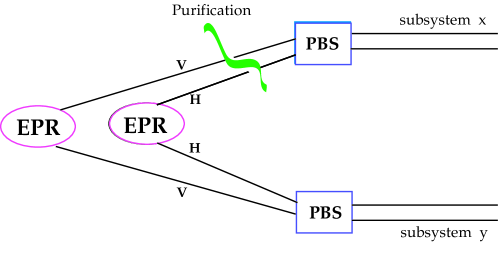
Figure 1: Scheme for transforming quadrature entanglement into continuous variable polarization entanglement. Two quadrature entangled pairs, with different polarizations $H$ and $V$, are sent to polarizing beam splitters (PBS). The emerging beams are then used to measure Stokes operators in the two subsystems $x$ and $y$. Local operations on the subsystem $x$, prior mode mixing at PBS, allow for entanglement purification.

We assume that the two horizontally and the two vertically polarized inputs are intense entangled pairs with fluctuations described by two-mode squeezed vacuum states [10]

$$|\psi\rangle_{H_{x}H_{y}V_{x}V_{y}}=\sum_{n=0}^{\infty}c_{n}|n,n\rangle_{H_{x}H_{y}}\sum_{m=0}^{\infty}c_{m}|m,m\rangle_{V_{x}V_{y}}\,,$$ (4)

where $c_{n}=\lambda^{n}\sqrt{1-\lambda^{2}}$ with $\lambda$ the two-mode squeezing parameter [10] (for the sake of simplicity we assume $\lambda$ equal for both pairs). If we introduce the amplitude and phase quadrature operators

$${\hat{X}}^{+}_{j}={\hat{a}}_{j}+{\hat{a}}^{{\dagger}}_{j}\,,\qquad{\hat{X}}^{-}_{j}=-i\left({\hat{a}}_{j}-{\hat{a}}^{{\dagger}}_{j}\right)\,,\qquad(j=H\,,\,V)\,,$$ (5)

it is easy to see [10] that for $\lambda\to 1$ each pair of eq.(4) tends to be a maximally entangled state, like the EPR state [11], for it results simultaneous eigenstate of the difference of amplitude quadrature fluctuations $\delta{\hat{X}}^{+}_{j_{x}}-\delta{\hat{X}}^{+}_{j_{y}}$ ($j=H,V$) and of the sum of phase quadrature fluctuations $\delta{\hat{X}}^{-}_{j_{x}}+\delta{\hat{X}}^{-}_{j_{y}}$ (we have used the notation $\hat{O}=\langle\hat{O}\rangle+\delta\hat{O}$). For this reason such entanglement is usually refered as quadrature entanglement.

Since we have assumed bright input beams, the Stokes operators (1) and (2) can be rewritten as

$${\hat{S}}_{0} = \alpha_{H}^{2}+\alpha_{V}^{2}+\alpha_{H}\,\delta{\hat{X}}^{+}_{H}\,,$$ (6)

$${\hat{S}}_{1} = \alpha_{H}^{2}-\alpha_{V}^{2}+\alpha_{H}\,\delta{\hat{X}}^{+}_{H}-\alpha_{V}\,\delta{\hat{X}}^{+}_{V}\,,$$ (7)

$${\hat{S}}_{2} = 2\alpha_{H}\alpha_{V}\cos\theta+\alpha_{H}\cos\theta\,\delta{\hat{X}}^{+}_{V}-\alpha_{H}\sin\theta\,\delta{\hat{X}}^{-}_{V}$$ (8)

$$+\alpha_{V}\cos\theta\,\delta{\hat{X}}^{+}_{H}-\alpha_{V}\sin\theta\,\delta{\hat{X}}^{-}_{H}\,,$$

$${\hat{S}}_{3} = -2i\alpha_{H}\alpha_{V}\sin\theta-i\alpha_{H}\sin\theta\,\delta{\hat{X}}^{+}_{V}-i\alpha_{H}\cos\theta\,\delta{\hat{X}}^{-}_{V}$$ (9)

$$-i\alpha_{V}\sin\theta\,\delta{\hat{X}}^{+}_{H}+i\alpha_{V}\cos\theta\,\delta{\hat{X}}^{-}_{H}\,,$$

where $\alpha_{j}=\langle a_{j}\rangle$ ($j=H,V$).

To provide a proper definition of the entanglement in terms of the operators (6)-(9), we use the general inseparability criterion proposed in [12]. Namely, starting from a generic couple of observables $\hat{A}$ and $\hat{B}$ for each subsystem with ${\hat{\cal C}}=i\left[{\hat{A}},{\hat{B}}\right]$, we construct the following observables on the total system

$${\hat{\cal U}} = r_{x}{\hat{A}}_{x}+r_{y}{\hat{A}}_{y}\,,\qquad r_{x},r_{y}\in{\bf R}\,,$$ (10)

$${\hat{\cal V}} = s_{x}{\hat{B}}_{x}+s_{y}{\hat{B}}_{y}\,,\qquad s_{x},s_{y}\in{\bf R}\,.$$ (11)

Then, a sufficient condition for inseparability reads

$$\Delta^{2}{\hat{\cal U}}+\Delta^{2}{\hat{\cal V}}<\left(\left|r_{x}s_{x}\right|\,\left|\langle{\hat{\cal C}}_{x}\rangle\right|+\left|r_{y}s_{y}\right|\,\left|\langle{\hat{\cal C}}_{y}\rangle\right|\right)\,,$$ (12)

where $\Delta^{2}\hat{O}=\langle\delta\hat{O}^{2}\rangle$. For the sake of simplicity we choose $r=\pm 1$ and $s=\pm 1$, then eq.(12) becomes

$$\Delta_{x\pm y}^{2}\hat{A}+\Delta_{x\pm y}^{2}\hat{B}<2\left|\langle\left[\delta\hat{A},\delta\hat{B}\right]\rangle\right|\,.$$ (13)

Here $\Delta\!_{x\pm y}^{2}\!\hat{O}$ is the smaller of the sum and difference variances of the operator $\hat{O}$ between beams $x$ and $y$, i.e. $\Delta\!_{x\pm y}^{2}\!\hat{O}\!=\!\min{\langle(\delta\hat{O}_{x}\!\pm\!\delta\hat{O}_{y})^{2}\rangle}$. To allow direct analysis of our results, we define the degree of inseparability $I_{{\hat{A}},{\hat{B}}}$, normalized such that $I_{{\hat{A}},{\hat{B}}}\!<\!1$ guarantees the state is inseparable

$$I_{{\hat{A}},{\hat{B}}}=\frac{\Delta\!_{x\pm y}^{2}\!\hat{A}+\Delta\!_{x\pm y}^{2}\!\hat{B}}{2|\langle[\delta\hat{A},\delta\hat{B}]\rangle|}$$ (14)

Following Ref. [8], we arrange the entanglement such that the mean value of the three Stokes operators are the same ($|\!\langle\hat{S}_{i}\rangle\!|\!=\!\alpha^{2}$). This leads to $\alpha_{V}^{2}\!=\!\frac{\sqrt{3}-1}{2}\alpha^{2}$, $\alpha_{H}^{2}\!=\!\frac{\sqrt{3}+1}{2}\alpha^{2}$, $\theta_{x}\!=\!\pi/4\!+\!n_{x}\pi/2$, and $\theta_{y}\!=\!\pi/4\!+\!n_{y}\pi/2$ where $n_{x}$ and $n_{y}$ are integers. By virtue of eq.(4), the two horizontally polarized inputs, and the two vertically polarized inputs, are quadrature entangled with the same degree of correlation such that $\Delta\!_{x\pm y}^{2}\!\hat{X}\!_{H}^{\pm}\!=\!\Delta\!_{x\pm y}^{2}\!\hat{X}\!_{V}^{\pm}\!=\!\Delta\!_{x\pm y}^{2}\!\hat{X}$. In this configuration, from eqs. (6)-(9) and (4) one also has $|\langle[\delta\hat{S}_{i}\delta\hat{S}_{j}]\rangle|=2\alpha^{2}$, for all $i\neq j$. To simultaneously minimize all three degrees of Stokes operator inseparability ($I_{{\hat{S}_{i}},{\hat{S}_{j}}}$) it is necessary that $\theta_{x}\!=\!-\theta_{y}\!+\!n\pi$. After making this assumption we find that $\Delta\!_{x\pm y}^{2}\!\hat{S}_{i}\!=\!\sqrt{3}\alpha^{2}\Delta\!_{x\pm y}^{2}\!\hat{X}$ for all $i$. Hence, in this situation $I_{{\hat{S}_{i}},{\hat{S}_{j}}}$ are all identical, and for any pair of Stokes operators the entanglement is the same, that is

$$I_{{\hat{S}}_{i},{\hat{S}}_{j}}(\lambda)=\sqrt{3}\left(\frac{1-\lambda}{1+\lambda}\right)\,,\qquad\forall i\neq j\,.$$ (15)

In principle it is possible to have all the three Stokes operators perfectly entangled. In other word, ideally the measurement of any Stokes operator of one of the beams, could allow the exact prediction of a different Stokes operator of the other beam (see fig. 1).

In fig. 2 it is shown the degree of inseparability (15) versus the two-mode squeezing parameter $\lambda$. It is worth noting that entanglement can only be recognized for approximately $\lambda>0.27$ while the state is entangled for any values $\lambda\neq 0$. That is, the Stokes operators are not optimal entangled witnesses, as they are not tangent to the set of separable states [13].

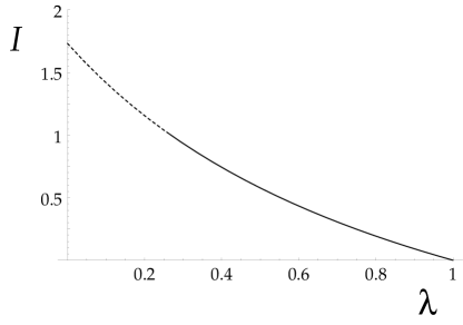
Figure 2: Degree of inseparability $I_{{\hat{S}}_{i},{\hat{S}}_{j}}(\lambda)$ vs $\lambda$. The dashed part of the line represents values above $1$.

Let us now consider the possibility to render the entanglement more “visible” (through polarization correlations) for low values of $\lambda$.

3 Entanglemet Purification

One important concept in quantum information theory is the entanglement purification (distillation) which allows the two parties to extract a small number of highly entangled, almost pure, states from a large number of weakly entangled mixed states [1]. These protocols involve only local operations and classical communication (LOCC) between the two parties; therefore they can be performed after the distribution of the entangled states (see fig. 1).

Since we are dealing with continuous variable, hereafter we shall consider the two relevant protocols developed till now [14, 15] which we label A and B respectively. They both involve nonlinear processes; as matter of fact it was recently proved the impossibility to purify Gaussian entangled states by means of Gaussian operations [16],

3.1 Scheme A

The scheme proposed by Duan et. al. [14] relies on nondemolition measurement of the total photon number in one of the two parties and represents a direct extension of the Schmidt projection method to infinite-dimensional Hilbert space. In this case, the nonlinearity required to implement a non-Gaussian transformation is induced by a measurement that should resolve the number of photons in one subsystem ($x$ in fig. 1).

Suppose the result of the measurement is $J$, then the state after measurement will be

$$|J\rangle_{H_{x}H_{y}V_{x}V_{y}}=\frac{1}{\sqrt{J+1}}\sum_{n=0}^{J}|n,n\rangle_{H_{x}H_{y}}|J-n,J-n\rangle_{V_{x}V_{y}}\,,$$ (16)

and the probability for the random outcome $J$ can be calculated from eqs.(4) and (16) as

$$\left|\langle\psi|J\rangle\right|^{2}=(J+1)\lambda^{2J}(1-\lambda^{2})^{2}\,.$$ (17)

Then, the degree of inseparability (14) calculated on the state (16) gives

$$I_{{\hat{S}}_{i},{\hat{S}}_{j}}(J)=\frac{\sqrt{3}}{J+1}\left[\sum_{m=0}^{J}\left(2m+1\right)-\sum_{m=0}^{J-1}\sqrt{\left(J-1\right)\left(m+1\right)}\right]\,,$$ (18)

which results independent of $\lambda$.

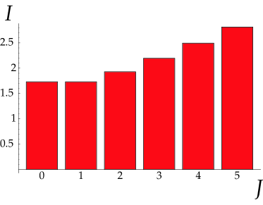
Figure 3: Degree of inseparability $I_{{\hat{S}}_{i},{\hat{S}}_{j}}(J)$ vs $J$.

Fig. 3 shows that $I_{{\hat{S}}_{i},{\hat{S}}_{j}}(J)$ never goes below $1$ (whatever is the value of $\lambda$). Hence the purification protocol does not succeed in improving the visibility of entanglement on polarization correlations, although the entanglement has been effectively enhanced [14].

3.2 Scheme B

The scheme proposed by Fiurasek [15] provides entanglement purification for any single copy of a two-mode squeezed vacuum state $\sum_{n}c_{n}|n,n\rangle$. The procedure in this case preserves the structure of a two-mode squeezed vacuum state, while the Schmidt coefficients $c_{n}$ are transformed to different ones, $c_{n}\to d_{n}$. The nonlinearity is provided by a cross Kerr interaction with an auxiliary mode prepared in a coherent state $|\alpha\rangle$ and undergoing a phase shift $\phi$. A subsequent eight-port homodyne detection of the auxiliary mode provides a random outcome $\beta\in{\bf C}$ (projection of the auxiliary mode onto a coherent state $|\beta\rangle$).

In this case the entanglement purification is described through the replacement

$$c_{n}\to d_{n}=\frac{\langle\beta|\alpha e^{in\phi}\rangle}{\sqrt{\pi Q(\beta)}}c_{n}\,,$$ (19)

where $Q(\beta)$ represents the probability density for the outcome $\beta$, that is

$$Q(\beta)=\frac{1}{\pi}\sum_{n=0}^{\infty}|\langle\beta|\alpha e^{in\phi}\rangle|^{2}\,|c_{n}|^{2}\,.$$ (20)

The degree of inseparability (14) prior the purification is given by eq.(15) and can be rewritten as

$$I\left(\lambda\right)=\sqrt{3}\sum_{n,m=0}^{\infty}\left[\left(2n+1\right)|c_{n}|^{2}|c_{m}|^{2}-2\left(n+1\right)|c_{m}|^{2}c_{n+1}c_{n}\right]\,,$$ (21)

so that after the purification it simply becomes

$$I\left(\beta\right)=\sqrt{3}\sum_{n,m=0}^{\infty}\left[\left(2n+1\right)|d_{n}|^{2}|d_{m}|^{2}-2\left(n+1\right)|d_{m}|^{2}d_{n+1}d_{n}\right]\,.$$ (22)

Then, we can introduce the entanglement increment by

$$\Gamma(\beta,\lambda)=\frac{E^{\prime}(\beta)}{E(\lambda)}\,,$$ (23)

where we have set

$$E^{\prime}(\beta)=\left\{\begin{array}[]{lll}1-I(\beta)\,,&&{\rm if}\;I(\beta)<1\\ 0\,,&&{\rm otherwise}\end{array}\right.\,,$$ (24)

as the degree of entanglement after the purification and

$$E(\lambda)=\left\{\begin{array}[]{lll}1-I(\lambda)\,,&&{\rm if}\;I(\lambda)<1\\ 0\,,&&{\rm otherwise}\end{array}\right.\,,$$ (25)

as the degree of entanglement prior the purification. Here, $\Gamma>1$ indicates the ability to recognize the entanglement improvement through the Stokes operators. The efficiency of the protocol can be defined as [17]

$$\Xi(\lambda)=1-\frac{1}{\Upsilon(\lambda)}\,,$$ (26)

where

$$\Upsilon(\lambda)=\frac{\int_{\Omega}d^{2}\beta\,Q^{2}(\beta)\Gamma(\beta,\lambda)}{\int_{\Omega}d^{2}\beta\,Q^{2}(\beta)}\,,$$ (27)

with $\Omega\equiv\{\beta\in{\bf C}|\Gamma(\beta)>1\}$. In eq.(27) we have used $Q^{2}$ as probability density because of two independent purification processes occur, one for each pair.

Figure 4: Efficiency of the purification protocol B vs $\lambda$.

In fig. 4 we show the efficiency of the protocol as function of the parameter $\lambda$. It takes its maximum for approximately $\lambda<0.27$ because, prior the purification, the Stokes‘ operators are not good enough operators to witness entanglement in this region of $\lambda$ and the purification protocol is efficient (see fig. 2). Obviously, the graph has a singular point in $\lambda=0$ where no entanglement is present at all. For $\lambda>0.27$ the protocol‘s efficiency rapidly decreases to zero because for these values of $\lambda$ the Stokes operators are good enough to recognize the entanglement present in the state (see fig. 2).

4 Conclusions

In conclusion, we have characterized two-party entanglement through polarization (Stokes operators) correlations. Stokes operators turn out to be useful in describing the transfer of quantum information from a freely propagating optical carrier to a matter system [6]. Furthermore, the use of continuous variable polarization entanglement combines the advantages of intense, easy to handle, sources of EPR-entangled light and efficient direct detection, thus opening the way to secure quantum communication with bright light [18]. However, we have shown that Stokes operators are not able to single out any level of entanglement from a given state. They well work when the degree of entanglement is high enough. Moreover, in order to make entanglement visible on polarization correlations, the purification should be accomplished with a suitable protocol.

The question whether one could ever recognize full entanglement with measurements of Stokes operators correlations could be addressed by optimizing the used entanglement criterion, or by exploring more sophisticated version of it [19]. This is planned for future work.

References

References

-
[1]
C. H. Bennett, G. Brassard, S. Popescu, B. Schumacher,
J. A. Smolin and W. K. Wooters,
Phys. Rev. Lett. 76, 722 (1996);
C. H. Bennett, H. J. Bernstein, S. Popescu and B. Schumacher, Phys. Rev. A 53, 2046 (1996). -
[2]
see e.g., Special Issue:
Quantum State Preparation and Measurement, J. Mod. Opt. 44, N.11/12 (1997);
D. G. Welsch, W. Vogel and T. Opatrny, Progress in Optics XXXIX, 63 (1999). -
[3]
M. D. Reid and P. Drummond,
Phys. Rev. Lett. 60, 2731 (1988);
L. M. Duan, G. Giedke, J. I. Cirac and P. Zoller, Phys. Rev. Lett. 84, 2722 (2000);
R. Simon, Phys. Rev. Lett. 84, 2726 (2000);
S. Mancini, V. Giovannetti, D. Vitali and P. Tombesi, Phys. Rev. Lett. 88, 120401 (2002). - [4] A. Aspect, P. Grangier and G. Roger, Phys. Rev. Lett. 49, 91 (1982).
-
[5]
N. V. Korolkova and A. S. Chirkin,
Journal of Modern Optics 43, 869 (1996);
A. S. Chirkin, A. A. Orlov and D. Yu Paraschuk, Kvant. Elektron. 20, 999 (1993);
A. P. Alodjants et al., Appl. Phys. B 66, 53 (1998);
T. C. Ralph, W. J. Munro and R. E. S. Polkinghorne, Phys. Rev. Lett. 85, 2035 (2000). -
[6]
J. Hald et al., Phys. Rev. Lett 83 1319 (1999);
B. Julsgaard et al., Nature 413, 400 (2001). - [7] N. Korolkova, G. Leuchs, R. Loudon, T. Ralph and C. Silberhorn, Phys. Rev. A 65, 052306 (2002).
-
[8]
W. P. Bowen, N. Treps, R. Schnabel and P. K. Lam,
Phys. Rev. Lett. 89, 253601 (2002);
W. P. Bowen, N. Treps, R. Schnabel, T. C. Ralph and P. K. Lam, J. Opt. B: Quantum Semiclass. Opt. 5, S467 (2003). - [9] B. A. Robson, Theory of Polarization Phenomena, (Clarendon Press, Oxford, 1974).
- [10] D. F. Walls and G. J. Milburn, Quantum Optics, (Springer, Berlin, 1995).
- [11] A. Einstein, B. Podolsky, N. Rosen, Phys. Rev. 47, 777 (1935).
- [12] V. Giovannetti, S. Mancini, D. Vitali and P. Tombesi, Phys. Rev. A 67, 022320 (2003).
-
[13]
see e.g.,
K. Eckert, O. Gühne, F. Hulpke, P. Hyllus, J. Korbicz, J. Mompart, D. Bruss, M. Lewenstein and A. Sanpera, in Quantum Information Processing, G. Leuchs and T. Beth Eds. (Wiley-VCH Verlag, Weinheim, 2003). - [14] L.-M. Duan, G. Giedke, J. I. Cirac and P. Zoller, Phys. Rev. Lett. 84, 4002 (2000); Phys. Rev. A 62, 032304 (2000).
- [15] J. Fiurasek, L. Mista Jr. and R. Filip, Phys. Rev. A 67, 022304 (2003).
-
[16]
J. Eisert, S. Scheel and M. B. Plenio,
Phys. Rev. Lett. 89, 137903 (2002);
J. Fiurasek, Phys. Rev. Lett. 89, 137904 (2002);
G. Giedke and J. I. Cirac, Phys. Rev. A 66, 032316 (2002). - [17] S. Mancini, Phys. Lett. A 279, 1 (2001).
-
[18]
T. C. Ralph, Phys. Rev. A 61, 010303(R) (2000);
62, 062306 (2000);
Ch. Silberhorn, N. Korolkova and G. Leuchs, Phys. Rev. Lett. 88, 167902 (2002). - [19] V. Giovannetti, arXiv:quant-ph/0307171.