About distillability of depolarized states

Abstract

Reduction criteria for distillability is applied to general depolarized states and an explicit condition is found in terms of a characteristic polynomial of the density matrix. 3 $\times$ 3 bipartite systems are analyzed in some details.

1 Introduction

Quantum information is mostly based on use of entanglement, and optimal performances of quantum protocols are obtained when the parties share maximally entangled states. However, entanglement is corrupted by the interaction with the environment, and it becomes crucial to establish whether or not quantum protocols may be exploited for a given level of the environmental noise. Quantum purification consists [1] in distilling a certain number of maximally entangled states from a larger number of corrupted states, i.e. to sacrifice some copies of the received state to increase the entanglement of others. Entanglement of partially corrupted states is only a necessary conditions for distillation, bound entanglement being the entanglement that cannot be distilled [2]. Some sufficient criterion for distillability has been proposed, the most relevant being the Reduction Criterion (RC) [3], and the norm-related criterions [4].

In this paper we apply the RC to a generalized class of depolarized states in $d$ dimensions. First we briefly review the distillability criterion and introduce a characteristic polynomial for our class of states. Then we apply our results to $3\times 3$ bypartite systems and numerically study the distillability.

2 The Reduction Criterion

We consider $d\times d$ bipartite systems. RC for distillability is based on map theory [3] and states that the negativity of the matrix

$$\rho_{A}\otimes I-\rho\leq 0,$$ (1)

where $\rho$ is the systems’s density operator and $\rho_{A}=\hbox{Tr}_{\!B}{\rho}$ is the reduced density operator, implies the distillability of the original density matrix $\rho$. Using RC we will study the distillability of depolarized states of the form

$$\rho=p\,|\psi\rangle\!\langle\psi|+\frac{1-p}{d^{2}}\,\mathbb{I}\>,$$ (2)

where $|\psi\rangle=\sum_{i}{a_{i}|ii\rangle}$ is a generic pure state. We already considered the Schmidt’s decomposition of $|\psi\rangle$ and thus, without loss of generality, the $a_{i}$’s are supposed to be real numbers, with the additional condition $\sum_{i}a_{i}^{2}=1$ [5]. $\mathbb{I}=\sum_{i,j}|ij\rangle\!\langle ji|$ denotes the $d\times d$ identity matrix. Depolarized maximally entangled state are obtained for $|\psi\rangle=\sum_{i}{\frac{1}{\sqrt{d}}|ii\rangle}$

To make the RC (1) of some computational use, we have to explicitly write down the $d^{2}\times d^{2}$ dimensional real matrix representing (2). In order to do this we first find out the Fock representation of (1) if $\rho$ is given by (2). We have:

$$\rho_{A}\otimes\mathbb{I}-\rho=\sum_{i,j}\left\{p\left(\,a_{i}^{2}|ij\rangle\!\langle ji|-a_{i}a_{j}|ii\rangle\!\langle jj|\right)+\frac{(d-1)(1-p)}{d^{2}}|ij\rangle\!\langle ji|\right\}$$ (3)

or, in matrix form:

$$\rho_{A}\otimes\mathbb{I}-\rho\,=\,p\,\left(\begin{array}[]{cccc}\mathbf{A}_{11}&\mathbf{A}_{12}&\cdots&\mathbf{A}_{1d}\\ \mathbf{A}_{21}&\mathbf{A}_{22}&\cdots&\mathbf{A}_{2d}\\ \vdots&&\ddots&\vdots\\ \mathbf{A}_{d1}&\cdots&\cdots&\mathbf{A}_{dd}\end{array}\right)+f_{d}(p)\,\mathbb{I}_{d^{2}\times d^{2}},$$ (8)

where the $\mathbf{A}$’s are $d\times d$ matrices given by

$$\mathbf{A}_{ii}=a_{i}^{2}\left(\mathbb{I}-\mathbb{D}[i,i]\right)\qquad\mathbf{A}_{ij}=-a_{i}a_{j}\mathbb{D}[i,j]\qquad\mathbf{A}_{ji}=\mathbf{A}_{ij}^{\mathrm{T}}\>,$$ (9)

and $f_{d}(p)\,=\,\frac{(d-1)(1-p)}{d^{2}}$. In Eqs. (9) $\mathbb{D}[i,j]$ denotes a matrix which is zero everywhere except for the $(i,j)$ entry, which is one. We are now in the position to write the characteristic polynomial $\mathbb{P}_{d}$ of the matrix (8) as a product of two terms

$$\mathbb{P}_{d}=\mathrm{P}_{d}(x)\,\prod_{i=1}^{d}\left(f_{d}(p)-\lambda+p\,a_{i}^{2}\right)^{d-1}\>,$$ (10)

where, using the substitution $x=f_{d}(p)-\lambda$, we have

$$\mathrm{P}_{d}(x)\,=\,x^{d}-\sum_{i=0}^{d-2}\left(d-i-1\right)\,p^{d-i}\,A_{d-i}^{d}\,x^{i}\>,$$ (11)

with

$$A_{k}^{d}=\sum_{j=0}^{d-k}A_{k-1}^{d-j-1}\,\left(A_{1}^{d-j}-A_{1}^{d-j-1}\right)\qquad A_{1}^{d}=\sum_{l=1}^{d}a_{l}^{2}\>.$$ (12)

Notice that the eigenvalues given by the second factor in (10) are always positive. Therefore, the sign of $\mathbb{P}_{d}$ is determined by (11). Notice also that in (11) the term $x^{d-1}$ is always missing.

2.1 Miscellaneous limits

As a first application we consider the case $a_{i}=d^{-1/2}$, e.g. when $|\psi\rangle$ is a maximally entangled state. The polynomial (11) reduces to

$$\mathrm{P}_{d}(x)|_{a_{i}=d^{-1/2}}=-\frac{1}{d^{d}}(p+d\,x)^{d-1}((d-1)p-d\,x).$$ (13)

The only relevant eigenvalue is the one given by the last factor of the $\mathrm{P}$ polynomial, namely

$$\lambda=-\frac{1-d}{d^{2}}+\frac{1-d^{2}}{d^{2}}\,p,$$ (14)

that yields the already known condition [3] $p\geq\frac{1}{d+1}$ for distillability of depolarized maximally entangled states.

As a second check consider the case of a $(d-j)$-dimensional maximally entangled state in a $d$-dimensional space, i.e. $a_{i}=1/\sqrt{(d-j)}$, $i=1,...,d-j$ while the remaining $j<d$ coefficients $a_{i}$ are set to zero. In this case it’s not difficult to see that the $d$-dimensional $\mathrm{P}$ polynomial (11) reduces to the $(d-j)$-dimensional one

$$\mathrm{P}_{d-j}(x)=\,-(d-j)^{-(d-j)}(p+(d-j)x)^{d-j-1}((d-j-1)p-(d-j)x)\>.$$ (15)

The non-trivial root of (15) reads

$$x=f_{d}(p)-\lambda=\frac{d-j-1}{d-j}\>,$$ (16)

leading to the condition

$$p\geq\frac{(d-1)(d-j)}{(d^{2}-1)(d-j)-d\,j}\>.$$ (17)

For example, for a $3\times 3$ system and a state with one zero-coefficient we find that the distillability is assured for $p>4/13$. Notice that RC is only a sufficient condition for distillability and therefore the bound in (17) need not to be a lower bound. Indeed, for the $3\times 3$ case considered above the system is also distillable for $p>2/11$ [6].

3 The $3\times 3$ dimensional bipartite system

As a further example we apply this representation to the case of a $3\times 3$ bipartite system. In this section, since $d$ is set to 3, we rename $A_{i}^{3}\equiv B_{i}$. Equation (8) becomes:

$$\rho_{A}\otimes\mathbb{I}-\rho\, = \,p\,\left(\begin{array}[]{ccccccccc}0&0&0&0&-a_{1}a_{2}&0&0&0&-a_{1}a_{3}\\ 0&a_{1}^{2}&0&0&0&0&0&0&0\\ 0&0&a_{1}^{2}&0&0&0&0&0&0\\ 0&0&0&a_{2}^{2}&0&0&0&0&0\\ -a_{1}a_{2}&0&0&0&0&0&0&0&-a_{2}a_{3}\\ 0&0&0&0&0&a_{2}^{2}&0&0&0\\ 0&0&0&0&0&0&a_{3}^{2}&0&0\\ 0&0&0&0&0&0&0&a_{3}^{2}&0\\ -a_{1}a_{3}&0&0&0&-a_{2}a_{3}&0&0&0&0\end{array}\right)$$ (28)

$$+\frac{2}{9}\,(1-p)\,\mathbb{I}_{9\times 9}.$$

The polynomial (11) now reads:

$$\mathrm{P}_{3}(x)\,=\,x^{3}-(d-2)\,p^{2}\,B_{2}\,x-(d-1)\,p^{3}\,B_{3}$$ (29)

with

$$\begin{array}[]{lcr}B_{2}=a_{1}^{2}a_{2}^{2}+a_{1}^{2}a_{3}^{2}+a_{2}^{2}a_{3}^{2}&\phantom{0.5cm}&B_{3}=a_{1}^{2}a_{2}^{2}a_{3}^{2}\end{array}$$ (31)

The solutions of (29) are:

$$x_{1} = 2\,p\,\sqrt{\frac{B_{2}^{3}}{3}}\,\cos\left[\frac{1}{3}\,\arctan\left(\sqrt{\frac{B_{2}^{3}}{27\,B_{3}^{2}}-1}\right)\right]$$ (32)

$$x_{\pm} = -p\,\sqrt{\frac{B_{2}^{3}}{3}}\,\left\{\cos\left[\frac{1}{3}\,\arctan\left(\sqrt{\frac{B_{2}^{3}}{27\,B_{3}^{2}}-1}\right)\right]\right.$$ (33)

$$\,\pm\left.\sqrt{3}\,\sin\left[\frac{1}{3}\,\arctan\left(\sqrt{\frac{B_{2}^{3}}{27\,B_{3}^{2}}-1}\right)\right]\right\}$$

and the nontrivial eigenvalues of (28) are:

$$\lambda_{i} = \frac{2}{9}\,(1-p)-x_{i}\,\,,\,i=1,+,-\>.$$ (34)

We are now in the condition to find out for which values of $p$ at least one (if any) of the nontrivial eigenvalues is negative. To this end, we switch to spherical coordinates, setting $a_{1}\rightarrow\sin\theta\,\sin\phi\$, $a_{2}\rightarrow\cos\theta\,\sin\phi\$, $a_{3}\rightarrow\cos\phi$, and plot the minimum value of $p$ for which (1) is satisfied, as a function of $\theta$ and $\phi$. Doing this for every eigenvalue (34), we than select the minimum value of $p$ between the three, at any given point on the plane $(\theta,\phi)$. It turns out that the only contributing eigenvalue is $\lambda_{1}$. Our results are plotted in Fig. 1.

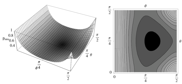
Figure 1: 3D and contour plots of the minimum $p$ satisfying RC as a function of state’s coefficients written in polar coordinates.

4 Conclusions

In this paper we have explicitly written the characteristic equation coming from the application of the Reduction Criterion for distillability to a class of one parameter generalized depolarized $d\times d$ bipartite states. The method has been applied to $3\times 3$ bipartite systems and the minimum value of the parameter $p$ that guarantees distillability has been found.

References

• [1] D. Deutsch et al., Phys. Rev. Lett. 77, 2818 (1996); C. H. Bennet et al., Phys. Rev. Lett. 76, 722 (1996); Horodecki et al., Phys. Rev. Lett. 78, 574 (1997);
• [2] A. Peres, Phys. Rev. Lett. 77, 1413 (1996); P. Horodecki, Phys. Lett. A 232, 333 (1997); D.P. DiVincenzo et al., Phys. Rev. A 61, 062312 (2000).
• [3] M. Horodechi, P. Horodecki, Phys. Rev. A 59, 4206 (1999).
• [4] K. Chen, L. Wu, Quant. Inf. and Comp. 3, 3 (2003) 193-202; O. Rudolph, quant-ph/0202121; M. Horodecki et al., quant-ph/0206008; H. Fan, quant-ph/0210168.
• [5] E. Schmidt, Math. Ann 63, 433 (1906).
• [6] G. Vidal, R. Terrac, Phys. Rev. A 59, 141 (1999).