Observation of Robust Quantum Resonance Peaks in an Atom Optics Kicked Rotor with Amplitude Noise

Abstract

The effect of pulse train noise on the quantum resonance peaks of the Atom Optics Kicked Rotor is investigated experimentally. Quantum resonance peaks in the late time mean energy of the atoms are found to be surprisingly robust against all levels of noise applied to the kicking amplitude, whilst even small levels of noise on the kicking period lead to their destruction. The robustness to amplitude noise of the resonance peak and of the fall–off in mean energy to either side of this peak are explained in terms of the occurence of stable, $\epsilon$–classical dynamics [S. Wimberger, I. Guarneri, and S. Fishman, Nonlin. 16, 1381 (2003)] around each quantum resonance.

I Introduction

The sensitivity of coherent quantum phenomena to the introduction of extraneous degrees of freedom is well documented Bundle1 . In particular, the coupling of a quantum system to its environment or, equivalently, subjection of the system to measurement is known to result in decoherence, that is, a loss of quantum interference phenomena.

The experimental study of decoherence ideally requires a system whose coupling to the environment may be completely controlled. The discipline of Atom Optics allows the realisation of this requirement in the form of atoms interacting with a far detuned optical field. The Atom Optics Kicked Rotor (AOKR), first implemented experimentally by the Raizen Group of Austin, Texas Moore1995 ; Raizen1996 , is a particular example of some interest as it is a quantum system which is chaotic in the classical limit. The AOKR is realised by subjecting cold atoms to short, periodic pulses of an optical standing wave detuned from atomic resonance. The atoms typically experience curtailed energy growth (dynamical localisation) Fishman1982 compared with the classical case, but may also experience enhanced growth for certain pulsing periods, an effect known as quantum resonance Izrailev1979 .

Previous AOKR experiments have shown that spontaneous emission events and noise applied to the amplitude of the kicking pulse train result in the destruction of quantum dynamical localisation NelsonPRL ; Raizen1998a . It might then be expected that the other well known signature of quantum dynamics in the AOKR, quantum resonance, should exhibit great sensitivity to spontaneous emission or noisy pulse trains. However, recent experiments by d’Arcy et al. have shown that detection of quantum resonance behaviour is actually enhanced in the presence of spontaneous emission dArcy2001 ; dArcy2001b ; dArcy2003pp , in stark contrast to the accepted wisdom on the effects of spontaneous emission noise. Recent numerical work has also focussed on the susceptibility of quantum resonance behaviour to applied noise Brouard2003 .

Here we present further experimental evidence of the robustness of the quantum resonance peak to certain types of noise. In this case, noise is added to the kicked rotor system by introducing random fluctuations in the amplitude or period of the optical pulses used to kick the atoms (collectively termed pulse train noise). We find that even in the presence of maximal amplitude noise, the structure near to quantum resonance persists (including the low energy levels to either side of the peak). This resistance to amplitude fluctuations runs counter to the expectation that quantum phenomena are sensitive to noise. In contrast, a small amount of noise added to the period of the pulses is enough to completely wash out the resonance structure. The robustness of the near resonant behaviour to amplitude noise is reminiscent of recent observations of quantum stability in the quantum kicked accelerator by Schlunk et al. Schlunk2003a ; Schlunk2003b .

The remainder of this paper is arranged as follows: Section II provides background on the formal AOKR system with amplitude and period noise. Section III reviews the study of quantum resonances in the kicked rotor. Our experimental procedure and results are found in Sections IV and V respectively, and the results are explained in Section VI in terms of the recently developed $\epsilon$–classical model for quantum resonance peaks. SectionVII offers conclusory remarks.

II Atom optics kicked rotor with amplitude and period noise

The Hamiltonian for an AOKR kicked with period $T$ with fluctuations in the amplitude and/or pulse timing is given in scaled units by

$$\hat{H}=\frac{\hat{\rho}^{2}}{2}-\kappa\cos(\hat{\phi})\sum^{N}_{n=0}R_{A,n}f(\tau-nR_{P,n}),$$ (1)

where $\hat{\phi}$ and $\hat{\rho}$ are the quantum operators for the (scaled) atomic position and momentum, respectively, $\kappa$ is the kicking strength, $f$ is the pulse shape function, $\tau=t/T$ is the scaled time and the terms $R_{A,n}$ and $R_{P,n}$ introduce random fluctuations in the amplitude and kicking period respectively. We also note the scaled commutator relationship $[\hat{\phi},\hat{\rho}]=i\mathchar 22\relax\mkern-9.0muk$, where $\mathchar 22\relax\mkern-9.0muk=8\omega_{r}T$ is a scaled Planck’s constant and $\omega_{r}$ is the frequency associated with the energy change after a single photon recoil for Caesium. The scaled momentum $\hat{\rho}$ is related to the atomic momentum $\hat{p}$ by the equation $\hat{\rho}/\mathchar 22\relax\mkern-9.0muk=\hat{p}/(2\hbar k_{L})$, where $k_{L}$ is the wave number of the laser light. In this paper, as in Refs. Auckland2003 ; dArcy2001 , momentum is presented in the “experimental units” of $\hat{p}/(2\hbar k_{L})$.

Assuming, for simplicity, a rectangular pulse shape, the stochasticity parameter $\kappa$ is related to experimental parameters by the equation

$$\kappa=\Omega_{\rm eff}\omega_{r}T\tau_{p},$$ (2)

where $\Omega_{\rm eff}$ is the potential strength created by the laser field, and $\tau_{p}$ is the duration of the kicking pulse. $\Omega_{\rm eff}$ is given by

$$\Omega_{{\rm eff}}=\frac{\Omega^{2}}{\Delta},$$ (3)

where $\Omega$ is the resonant, single beam Rabi frequency of the atoms and $\Delta$ (which is $\approx 2\times 10^{9}$ rad ${\rm s}^{-1}$ for these experiments) takes into account the relative transition strengths between and laser detunings from the different hyperfine states of caesium, as discussed in our previous papers (see, for example, NelsonPRL ; Auckland2003 ).

Noise is introduced by the terms $R_{i,n}=1+\delta_{i,n}$, where $\delta_{i,n}$ is a random variable with probability distribution

$$P(\delta_{i,n})=\left\{\begin{array}[]{ll}1/{\rm\mathcal{L}_{i}},&|\delta_{i,n}|<{\mathcal{L}_{i}/2}\\ 0,&\rm{else}\end{array}\right.$$ (4)

with $i=A$ denoting amplitude noise, and $i=P$ denoting period noise. The noise level is denoted $\mathcal{L}_{i}$. For amplitude noise, we have $0\leq{\mathcal{L}_{A}}\leq 2$, where a noise level of $2$ corresponds to the case where the kicking strength can vary between $0$ and $2\overline{\kappa}$ for each pulse, with $\overline{\kappa}$ the mean value of the kicking strength in the experiment. For period noise, $0\leq{\mathcal{L}_{P}}<{\mathcal{L}_{P,{\rm max}}}$ where ${\mathcal{L}_{P,{\rm max}}}$ is $1$ for the $\delta$-kicked rotor and $1-\alpha$ for the pulse kicked rotor in our experiments, with $\alpha$ the ratio of the pulse width to the pulse period (less than $1\%$ in our experiments). We note that our implementation of period noise differs from that used in RaizenPeriod in that it shifts each pulse a random amount from its zero–noise position rather than randomising the timing between consecutive pulses. This means that the effect of the period noise fluctuations is not cumulative (as it is in the aforementioned reference), allowing a more instructive comparison of the effects of period noise with those of amplitude noise.

III The quantum resonances of the AOKR

In a fully chaotic driven system no stable periodic orbits exist in phase space and thus no frequency of the driving force gives rise to resonant behaviour. Although the classical kicked rotor retains kick–to–kick correlations for any value of the stochasticity parameter, for sufficiently high $\kappa$ the phase space is essentially chaotic, and the dynamics are independent of the kicking period of the system. However, this is not true of the quantum system, even for large $\kappa$, as fundamental periodicities exist in the quantum dynamics. This may be seen by inspecting the one kick evolution operator for the quantum $\delta$–kicked rotor, which has the form

$$\hat{U}=\exp({\rm i}\kappa\cos\hat{\phi}/\mathchar 22\relax\mkern-9.0muk)\exp(-{\rm i}\hat{\rho}^{2}/(2\mathchar 22\relax\mkern-9.0muk)),$$ (5)

For the analysis of quantum resonance, the second exponential term (or free evolution term) of Eq. 5 is of primary importance. We see that if $\mathchar 22\relax\mkern-9.0muk$ is an even multiple of $2\pi$, and the state undergoing evolution is a momentum eigenstate (or a quantum superposition of such eigenstates) $|n\rangle$ such that $\hat{\rho}|n\rangle=n\mathchar 22\relax\mkern-9.0muk|n\rangle$, this term becomes unity. This is the quantum resonance condition, and it may be shown that atoms initially in momentum eigenstates undergo ballistic motion Izrailev1979 at resonant values of $\mathchar 22\relax\mkern-9.0muk$. For $\mathchar 22\relax\mkern-9.0muk=2\pi(2m-1)$, $m$ a positive integer, initial momentum eigenstates with even and odd $n$ acquire quantum phases after free evolution of $+1$ and $-1$ respectively. It is found that the additional possibility of $-1$ for the phase of odd momentum components of the wavefunction leads to oscillations in the mean energy of the kicked atomic ensemble Oskay2000 ; Deng1999 . Thus, $\mathchar 22\relax\mkern-9.0muk=2\pi$ is termed a quantum antiresonance.

We note that whilst quantum resonances are predicted to exist for all rational multiples of $\mathchar 22\relax\mkern-9.0muk=2\pi$, resonance peaks have only been observed in experiments and simulations at integral multiples. In this paper, we focus on the behaviour at $\mathchar 22\relax\mkern-9.0muk=2\pi$ and $\mathchar 22\relax\mkern-9.0muk=4\pi$ and will refer to the energy peaks at these values of the scaled Planck’s constant as the first and second quantum resonances respectively.

For a cloud of Caesium atoms at $5\mu$K, as used in our experiments, the atomic momentum distribution has a standard deviation of $\sim 5\hbar k_{L}$, so only a small momentum subclass of the atoms may be considered to be in an initial momentum eigenstate. In general, each atom has a momentum of the form $\rho=n+\beta$ (in scaled units), where $n$ is an integer and $\beta\in[0,1)$ is known as a quasimomentum. The appropriate evolution operator when the quasimomentum of the atoms is included is

$$\hat{U}_{\beta}=\exp({\rm i}\kappa\cos\hat{\phi}/\mathchar 22\relax\mkern-9.0muk)\exp(-{\rm i}(\hat{n}+\beta)^{2}/(2\mathchar 22\relax\mkern-9.0muk)).$$ (6)

For some values of quasimomenta, this one–kick evolution operator still exhibits the periodicity necessary for resonance Wimberger2003 . Specifically, ballistic energy growth occurs for $\mathchar 22\relax\mkern-9.0muk=2\pi$, $\beta=0.5$ and for $\mathchar 22\relax\mkern-9.0muk=4\pi$, $\beta=0$ or $0.5$.

The quantum resonances of the AOKR were first studied experimentally by the group of Mark Raizen at Austin, Texas Moore1995 ; Raizen1996 ; Oskay2000 . In particular, ref. Moore1995 presented the results of experiments in which the momentum distribution of the atoms was recorded for various kicking periods. The momentum distributions corresponding to quantum resonance were found to be narrower than those off resonance. The relatively small population of atoms undergoing ballistic energy growth at resonance was not detected experimentally and no difference was found between momentum distributions for odd and even multiples of $\mathchar 22\relax\mkern-9.0muk=2\pi$. In ref. Oskay2000 a further study by the group detected the expected ballistic peaks at $\mathchar 22\relax\mkern-9.0muk=2\pi$ and $\mathchar 22\relax\mkern-9.0muk=4\pi$. Additionally, small oscillations in the widths of the atomic momentum distributions as a function of kick number were seen only at $\mathchar 22\relax\mkern-9.0muk=2\pi$ – a result of the anti-resonance behaviour described earlier.

More recent experiments by d’Arcy et al. dArcy2001 ; dArcy2001b ; dArcy2003pp have focussed on the effect of spontaneous emission on the quantum resonance peaks. They found experimentally that spontaneous emission makes these peaks more prominent – a somewhat counter–intuitive result. Further theoretical investigations revealed that this phenomenon was due to the reshuffling of atomic quasimomenta caused by spontaneous emission which allows more atoms to experience resonant behaviour at some time during their evolution. Additionally, reshuffling of quasimomenta results in fewer atoms gaining large momenta from multiple resonant kicks. Without spontaneous emission, resonant atoms soon travel outside the finite observation window of the experiment and thus do not contribute to the measured energy of the atomic ensemble.

Our experiments measure the structure of the mean energy around the quantum resonance peak in a similar fashion to the experiments described above. The pulse period is scanned over the resonant value and the mean energy is extracted from the measured momentum distributions at each value of $T$. For the power and detuning of the kicking laser used in this experiment, there is a constant chance of spontaneous emission per pulse of $\sim 2.5\%$. As in dArcy2001 , this is found to increase the height and width of the resonance peaks and make them more amenable to investigation. Our numerical studies show that the non-zero spontaneous emission rate does not affect the study of amplitude noise and period noise on the quantum resonance peak. This is because the mechanisms by which pulse train noise and spontaneous emission noise influence the atomic dynamics are totally different: Spontaneous emission events affect individual atoms by changing their quasimomenta; Amplitude and period noise change the kick–to–kick correlations over the entire atomic ensemble and do not change atomic quasimomenta. Thus the advantages of a relatively high spontaneous emission rate may be utilised without biasing the study of the effects of pulse train noise on the quantum resonance peaks.

IV Experimental setup

Our experiments utilise a $5$ $\mu$K cloud of cold Caesium atoms, provided by a standard six beam magneto–optical trap (MOT) Monroe1990 . The atoms interact with a pulsed, far-detuned optical standing wave which is created by retroreflecting the light from a 150mW (slave) diode laser which is injection locked to a lower power (master) diode laser. The output of the master laser may be tuned over a range of about $4$ GHz relative to the $6S_{1/2}(F=4)\rightarrow 6P_{3/2}(F^{\prime}=5)$ transition of the Caesium $\rm D_{2}$ line. The detuning of the laser from this transition is denoted $\delta$. The frequency of the kicking laser is monitored by observing the spectrum of its beat signal with the trapping laser.

The standing wave has a horizontal orientation rather than the vertical orientation used in the quantum accelerator experiments of references Schlunk2003a ; Schlunk2003b . It is pulsed by optically switching the laser light using an acousto–optic modulator (AOM). The amplitude of the AOM’s driving signal is controlled by a programmable pulse generator (PPG) to achieve the desired pulse train shape. For amplitude noise experiments, the AOM’s response to the amplitude of its driving signal must first be calibrated, since the pulse heights need to be uniformly distributed. The PPG consists of a random access memory (RAM) chip which can store up to $2^{16}$ $12$ bit words representing samples of the pulse train. On receipt of a gate pulse, the samples in the RAM are read into a digital to analogue convertor at 25 MHz, corresponding to a 40ns temporal resolution for the pulse trains. A given realisation of a noisy pulse train (for amplitude or period noise) is created by using computer–generated pseudo–random numbers to give fluctuations about the mean amplitude or mean pulse position in a standard pulse train. The noisy pulse train is then uploaded to the PPG.

In a typical experimental run, the cooled atoms were released from the MOT and subjected to $20$ standing wave pulses, then allowed to expand for an additional free drift time in order to resolve the atomic momenta. The momentum resolution of our experiments for a $12$ms expansion time is $0.29$ $2$–photon recoils. After free expansion, the atoms were subjected to optical molasses, effectively freezing them in place, and a fluoresence image of their spatial distribution was taken. The timing of the experiment was controlled by sequencing software running on the $\rm RTLinux^{\tiny\texttrademark}$ operating system kernel giving worst case timing errors of $30$ $\mu$s RTLinuxFAQ , or $0.25\%$ of the atomic time of flight.

Some experimental imperfections have a systematic effect on our data and need to be taken into account in simulations in order for meaningful comparisons to be made. Firstly, when the standing wave is on, individual atoms experience differing potentials depending on their radial position in the beam, due to the gaussian mode shape of the beam. This can affect the experimental resolution of the multi–peaked ‘diffusion resonance’ structure in the mean energy which occurs between primary quantum resonances, as this structure is strongly dependent on the exact potential strength Auckland2003 ; Daley2001 . However it is not so critical to the observation of quantum resonance peaks, due to the very resistance to variations in amplitude discussed in this paper. Nonetheless, this spread in kicking strengths is taken into account in our simulations. Secondly, in order to achieve a spontaneous emission rate sufficiently high to make the quantum resonance peaks prominent and amenable to study, a detuning from resonance of about $500$ MHz was used in our experiments. This value of the detuning is large enough to ensure the condition $\delta\gg\overline{\Omega}$ (where $\overline{\Omega}$ is the average atomic Rabi frequency taken over the different hyperfine transitions) which is assumed in the derivation of the AOKR Hamiltonian Graham1992 . However, the difference in detuning between the $F=4$ ground state and each of the hyperfine excited states $F^{\prime}=3,4,5$, as well as the difference in coupling strengths between magnetic substates, leads again to a spread in kicking strengths (as detailed in reference Auckland2003 ). Once again, this effect is allowed for in our simulations.

We also note that the application of amplitude and period noise to our pulse trains inherently creates random scatter in our data since each different noise realisation gives rise to a different mean energy. Thus, meaningful results may only be obtained by averaging the energy from a number of separate experiments with different noise realisations. For experiments where the noise is solely a result of spontaneous emission events, the statistics are already excellent, since the mean energy is calculated for a large number of individual atoms. This is not true for pulse train noise experiments which affect correlations over the entire atomic ensemble. Each point on our curves represents an average of 12 separate experiments (except in the zero noise case, where 3 repetitions was found to be sufficient). This number of repetitions reduces the error to a size such that any quantum resonance structure may be confidently identified.

V Experimental and simulation results

We now present experimental measurements of the quantum resonance peaks at $\mathchar 22\relax\mkern-9.0muk=2\pi$ and $4\pi$, in the presence of noise applied to the amplitude or period of the kicking pulse train(Figs. 1 and 2). Simulations are performed using the Monte Carlo wavefunction method as has previously been discussed in refs. Daley2001 ; Auckland2003 . For comparison with simulations, the value of $T$ corresponding to quantum resonance (that is $\mathchar 22\relax\mkern-9.0muk=2\pi$ or $4\pi$) is taken to be the experimental position of the resonance peak. This gives values of $T_{{\rm res},1}=61\mu$s and $T_{{\rm res},2}=121.5\mu$s which are within $1\%$ of the theoretical values of $2\pi/8\omega_{r}=60.5\mu$s and $4\pi/8\omega_{r}=121\mu$s respectively. The experimental resolution is limited by the spacing between consecutive values of $T$ (i.e. $0.5\mu$s). However, the exact position of the quantum resonances is not important to the results presented here which are concerned with the overall shape of the resonance peaks.

In this section, we measure the mean energy of the atomic ensemble, which is given by $E=<\hat{p}^{2}>/2(2\hbar k_{L})^{2}$. This quantity is referred to as the energy in 2 photon–recoil units. The height of the quantum resonance for a given number of kicks $n$ was found in reference Wimberger2003 to be $E_{\rm res}=(1/4)(\kappa/\mathchar 22\relax\mkern-9.0muk)^{2}n$. In the presence of amplitude noise, additional diffusive energy is gained which, for $\mathcal{L}_{A}=2$, is of size $(\kappa^{2}/12\mathchar 22\relax\mkern-9.0muk^{2})n$ Steck2000 . Thus, for maximal amplitude noise, the height of the quantum resonance energy peak is predicted to be

$$E_{\rm res}=\frac{1}{3}\left(\frac{\kappa}{\mathchar 22\relax\mkern-9.0muk}\right)^{2}n.$$ (7)

We use this equation to determine the value of $\kappa$ to be used in our amplitude noise simulations. Although this method systematically underestimates the true value of $\kappa$ (since small populations of resonant atoms with high momenta cannot be detected experimentally) it avoids the many systematic errors that arise when $\kappa$ is estimated from power measurements of the kicking beam outside the MOT chamber. The values of $\kappa$ gained from this equation are consistent with those estimated from experimental parameters.

If period noise is being applied instead, simulations show that the energy around the second quantum resonance saturates at the quasilinear value for the highest noise level, which is given by multiplying the quasilinear energy growth $\kappa^{2}/4\mathchar 22\relax\mkern-9.0muk^{2}$ Rechester1980 by the number of kicks to give

$$E_{\rm q.l.}=\frac{1}{4}\left(\frac{\kappa}{\mathchar 22\relax\mkern-9.0muk}\right)^{2}n.$$ (8)

Thus, having measured the height of the resonance for an amplitude noise level of $2$, we can solve Eq. (7) for $\kappa/\mathchar 22\relax\mkern-9.0muk$ which gives $3.77\pm 0.04$. Similarly, having calculated the experimental quasi–linear energy of $66\pm 0.7$ from the line fitted in Fig. 2(b), we can solve Eq. (8) for $\kappa/\mathchar 22\relax\mkern-9.0muk$ which gives $3.63\pm 0.03$. Given the different systematic errors which arise for amplitude and period noise calculations of $\kappa$ and the possibility of laser power drift between experimental runs, we do not expect perfect agreement between the two values. Using the values of $\kappa$ gained from Eqs. (7) and (8) in our simulations we find good quantitative agreement between experimental and simulation results. We note that period noise experiments allow $\kappa$ to be determined more accurately because the quantum resonance behaviour is destroyed and therefore the wings of the momentum distributions are not populated. This leads to more accurate values for the experimentally measured final energies.

Once $\kappa$ has been calculated from the measured energies, the spontaneous emission rate per pulse may be deduced by calculating the Rabi frequency $\Omega$ from Eqs.(2) and (3) and using the standard expression to find the probability of spontaneous emission Metcalf1999 . Measured and simulated energies are plotted against $\mathchar 22\relax\mkern-9.0muk$ (which may also be thought of as the scaled kicking period of the kicked rotor system (as in Wimberger2003 ) where $\mathchar 22\relax\mkern-9.0muk=2\pi$ corresponds to the kicking period at which the first quantum resonance peak occurs).

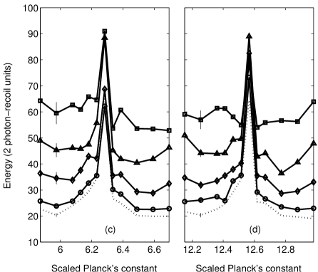
Figure 1: Measured energies ((a) and (b)) near the first and second primary quantum resonances and associated simulation results ((c) and (d)) for various levels of amplitude noise. We have taken $\kappa/\mathchar 22\relax\mkern-9.0muk=3.77$, as calculated from Eq. 7 and the spontaneous emission rate used for simulations is $2.5\%$. The dotted line represents the no-noise case, circles ${\mathcal{L}_{A}}=0.50$, diamonds ${\rm\mathcal{L}_{A}}=1.0$, triangles ${\mathcal{L}_{A}}=1.50$ and squares ${\mathcal{L}_{A}}=2.0$. Sample error bars are shown on the second point for each curve.

V.1 Amplitude noise

In our experiments, we measured energies at pulsing periods close to quantum resonance for the first and second quantum resonances, which occur at $\mathchar 22\relax\mkern-9.0muk=2\pi$ and $4\pi$ respectively. Amplitude noise was applied at levels of ${\mathcal{L}_{A}}=0.5,1,1.5$ and $2$. Fig. 1 shows the results obtained. We see that the resonance peak increases in height and that the reduced energy level to either side of resonance rises with increasing noise level. However, somewhat surprisingly, the resonance peak still remains prominent compared to the surrounding energies, even for the highest possible level of amplitude noise, although it becomes less well defined. We note that there is essentially no difference between the behaviour seen at the first and second quantum resonances apart from the fact that the energies are systematically lower for the second quantum resonance in experiments. This is due, in part, to the fact that the atomic cloud expands to a larger size during kicking for the second quantum resonance as compared with the first. This leads to a lower average kicking strength being experienced by the atoms (a feature not included in our simulations). Additionally, the total expansion time for the atoms, including kicking , is constant which means that for the sweeps over the second quantum resonance the atoms have less free expansion time after kicking than at the first quantum resonance. This also leads to a systematic underestimation of the energy.

That the dynamics at quantum resonance itself is robust against amplitude noise is not surprising. The resonance arises because the time between pulses matches the condition for unity quantum phase accumulation after free evolution. The introduction of amplitude noise does not affect this fundamental resonance criterion. Seen from the point of view of atom optics, the resonant period is the Talbot time (corresponding to $\mathchar 22\relax\mkern-9.0muk=4\pi$) dArcy2001 ; dArcy2001b . Whilst the amplitude of the pulses applied affects the number of atoms coupled into higher momentum classes, it does not affect the period dependent Talbot effect which gives rise to the characteristic energy growth seen at resonance.

The most surprising feature in these experiments is the survival of low energy levels to either side of the resonance. Persistence of quantum dynamical localisation is the most obvious explanation for the sharp decrease in energy to either side of quantum resonance. However the results of Steck et al. Steck2000 (which were performed far from quantum resonance at $\mathchar 22\relax\mkern-9.0muk=2.08$) demonstrated that dynamical localisation is destroyed by high levels (corresponding to $\mathcal{L}_{A}=2$) of amplitude noise. In Section VI, we will employ the recently developed $\epsilon$–classical description of the quantum resonance peak to explain this persistence of localisation.

We see that the experimentally measured resonance peaks are broader than those predicted by simulations. The broadening may result from a higher than expected spontaneous emission rate, resulting from a small amount of leaked molasses light which is inevitably present during the kicking cycle. Additionally, phase jitter on the optical standing wave can be caused by frequency instability of the kicking laser and mechanical vibrations of the retroreflecting mirror. Such phase noise is equivalent to a constant level of period noise and would also lead to broadening of the resonance. It is hard to quantify the amount of phase noise present, although the clear visibility of the resonances when no extra period noise is applied (see dotted line, Fig. 2) suggests that it is small in amplitude. However, these uncertainties do not affect the observation of the qualitative shape of the resonance structure under the application of amplitude noise and in particular, the puzzling robustness of the low energy levels to either side of resonance.

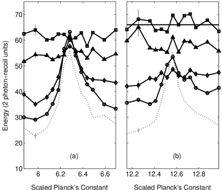
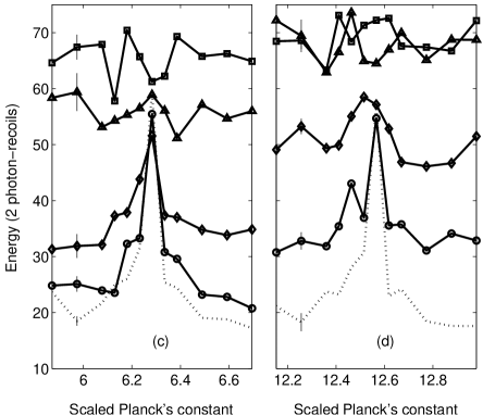
Figure 2: Measured energies ((a) and (b)) near the first and second primary quantum resonances and associated simulation results ((c) and (d)) for various levels of period noise. We have taken $\kappa/\mathchar 22\relax\mkern-9.0muk=3.61$, as calculated from Eq. 8 and the spontaneous emission rate used for simulations is $2.5\%$ The dotted line represents the no-noise case, circles ${\mathcal{L}_{P}}=0.01$, diamonds ${\mathcal{L}_{P}}=0.02$, triangles ${\mathcal{L}_{P}}=0.05$ and squares ${\mathcal{L}_{P}}=0.1$. Sample error bars are shown on the second point for each curve. In (b), a straight line was fitted to the energies in the highest noise case. It gives the quasi–linear energy as $66\pm 0.7$.

V.2 Period noise

For comparison, we also present results showing the effect of period noise on the first two primary quantum resonance peaks. It may be seen that even small amounts of this type of noise have a large effect on the near resonant dynamics. Fig. 2 shows the results for noise levels of $0.01$, $0.02$, $0.05$ and $0.1$. The first primary quantum resonance peak is found to be very sensitive to small deviations from strict periodicity of the pulse train. Noise levels of $0.05$ and $0.1$ completely wash out the peak, regaining the flat energy vs. kicking–period curve that we expect in the case of zero kick–to–kick correlations. The effect of period noise on the second primary quantum resonance is similar, although it is even more sensitive with an $0.02$ noise level completely destroying the peak. At higher noise levels, the mean energy tends towards the zero–correlation energy level.

The greater effect of period noise on the second quantum resonance is due to the greater absolute variation possible in the free evolution period between pulses, since the kicking period in this case is twice that of the first quantum resonance. This has been verified by our group in separate experiments where the absolute variation of the kicking period was held constant MarkThesis . Such noise was found to have a more uniform effect on structures in the mean energy. Sensitivity of the dynamics near quantum resonance to noise applied to the kicking period is not surprising, given the precise dependence of the resonance phenomenon on the pulse timing. The quantum phase accumulated between kicks is randomised and the kick–to–kick correlations destroyed. However, the stark contrast between the sensitivity of the near resonant dips in energy to amplitude and period noise requires further elucidation, which we now provide by looking at the correlations which lead to quantum resonance at early times and the $\epsilon$–classical dynamics of the kicked rotor near quantum resonance.

VI Reappearance of stable dynamics close to quantum resonance

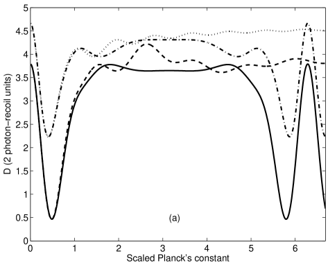
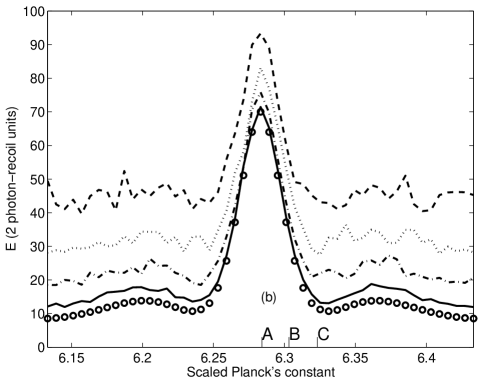
Figure 3: Analytical predictions of the effect of amplitude noise on the quantum resonance peak at $2\pi$ for $\kappa/\mathchar 22\relax\mkern-9.0muk=3.7$. (a) shows the behaviour of the early energy growth rate $D$ (as given by Eq. 10) of the classical and quantum kicked rotor as a function of $\mathchar 22\relax\mkern-9.0muk$ for amplitude noise levels of $\mathcal{L}_{A}=1$ and $2$. Dashed and dotted lines are the classical rates for amplitude noise levels of $1$ and $2$ respectively. Solid and dash-dotted lines are the quantum rates for $\mathcal{L}_{A}=1$ and $2$ respectively. (b) shows the resonant peak produced by 20 iterations of Eq. (12) about $\mathchar 22\relax\mkern-9.0muk=2\pi$ with ${\mathcal{L}_{A}}=0$ (circles), $0.5$ (solid line), $1.0$ (dash-dotted line), $1.5$ (dashed line) and $2.0$ (dotted line). Each point is an average of 10 different noise realisations. The letters A–C indicate values of $\epsilon$ as referenced from Fig. 4.

We now seek to explain the surprising resilience of the structure near quantum resonance to the application of amplitude noise. Since the effect of amplitude noise is the same for the resonance peaks at $\mathchar 22\relax\mkern-9.0muk=2\pi$ and $4\pi$ we consider only the resonance peak about $\mathchar 22\relax\mkern-9.0muk=2\pi$, although the arguments easily generalise to other quantum resonance peaks occuring at multiples of this value. We also limit our attention to the case where there is no spontaneous emission, as this form of decoherence, at the levels present in these experiments, merely broadens the resonance peak and does not affect its qualitative behaviour in the presence of amplitude noise.

The stability of the quantum resonance structure in the late time energy (as measured in our experiments) may be explained by appealing to the $\epsilon$–classical mechanics formulated by Wimberger et al. Wimberger2003 ; Wimberger2003bpp ; dArcy2003pp . In this description of the kicked rotor dynamics, a fictitious Planck’s constant is introduced which is referenced to zero exactly at quantum resonance. Thus, even though the quantum resonance peak is a purely quantum mechanical effect, its behaviour may be well described by a (fictitious) classical map near to resonance.

Before considering this picture, however, we will look at the resonances found in the early time classical and quantum energy growth rates of the kicked rotor which provide similar insight over a wider range of values for $\mathchar 22\relax\mkern-9.0muk$. The classical rates were first derived by Rechester and White Rechester1980 and their work was extended to the quantum kicked rotor by Shepelyansky Shepelyansky1987 . These expressions for the early time classical and quantum energy growth rate, $D$, have the advantage that they hold for any pulsing period and not just for those within an $\epsilon$ neighbourhood of the quantum resonance period. Fig. 3(a) plots the early–time energy growth rate $D$ for the classical and quantum dynamics against the effective Planck’s constant $\mathchar 22\relax\mkern-9.0muk$. For sufficiently large values of $\kappa/\mathchar 22\relax\mkern-9.0muk$ the energy growth rate after 5 kicks obeys the approximate expression Shepelyansky1987

$$D \approx \frac{1}{2}\left(\frac{\kappa}{\mathchar 22\relax\mkern-9.0muk}\right)^{2}\left(\frac{1}{2}-J_{2}(K)-J_{1}^{2}(K)\right.$$ (9)

$$\left.\frac{}{}+J_{2}^{2}(K)+J_{3}^{2}(K)\right),$$

where the $J_{n}$ are Bessel functions and $K=\kappa$ for the classical case and $K=\kappa_{q}=2\kappa\sin(\mathchar 22\relax\mkern-9.0muk/2)/\mathchar 22\relax\mkern-9.0muk$ for the quantum case. The energy growth rate is expressed in the same energy units used in reference Auckland2003 . This formula was generalised by Steck et al. Steck2000 to the case where amplitude noise is present in the system, giving

$$D \approx \frac{\kappa^{2}+\mathrm{Var}(\delta K)}{4\mathchar 22\relax\mkern-9.0muk^{2}}+\frac{\kappa^{2}}{2\mathchar 22\relax\mkern-9.0muk^{2}}\left(-\mathscr{J}_{2}(K)\right.$$ (10)

$$\left.\frac{}{}-\mathscr{J}_{1}^{2}(K)+\mathscr{J}_{2}^{2}(K)+\mathscr{J}_{3}^{2}(K)\right),$$

where $K$ is defined as before, $\delta K$ is a random variable giving the fluctuation in $K$ at each kick, $\mathrm{Var}(\delta K)$ is the variance of the noise distribution $P(\delta K)$ , and

$$\mathscr{J}_{n}(K):=\int_{-\infty}^{\infty}P(\delta K)J_{n}(K+\delta K){\rm{d}}(\delta K).$$ (11)

The new functions $\mathscr{J}_{n}$ are averages of the normal Bessel functions over the noise distribution. We note that references Steck2000 and Shepelyansky1987 deal with diffusion of the momentum $\rho$, whereas we present our results in terms of $\rho/\mathchar 22\relax\mkern-9.0muk$. Hence, when comparing our results for energies or energy growth rates with the formulae in the aforementioned references, division by $\mathchar 22\relax\mkern-9.0muk^{2}$ is necessary.

Of particular interest is the behaviour near $\mathchar 22\relax\mkern-9.0muk=0$. We note that using Shepelyansky’s formula in this regime can be problematic because in the fully scaled system, the width of the initial atomic momentum distribution scales with $\mathchar 22\relax\mkern-9.0muk$ and may become small enough that Shepelyansky’s assumption of a uniform initial momentum distribution is no longer valid Daley2002 . Assuming, however, that a broad initial momentum distribution may be maintained in the classical limit, we see that a peak exists at $\mathchar 22\relax\mkern-9.0muk=0$ for both the classical and quantum dynamics and the classical and quantum curves match perfectly until $\mathchar 22\relax\mkern-9.0muk\sim 0.5$. More importantly, a reduced energy region at $\mathchar 22\relax\mkern-9.0muk\approx 0.5$ remains even for the highest level of amplitude noise, as seen in Fig. 3(a). At larger values of $\mathchar 22\relax\mkern-9.0muk$, the oscillations in the classical growth rate are destroyed by noise. However, in the quantum case, the robust peak structure seen near $\mathchar 22\relax\mkern-9.0muk=0$ repeats itself at multiples of $\mathchar 22\relax\mkern-9.0muk=2\pi$. The survival of the structure near $\mathchar 22\relax\mkern-9.0muk=0$ is attributable to the near integrability of the dynamics (classical and quantum) for small values of $\mathchar 22\relax\mkern-9.0muk$. We recall that in the scaling used for these experiments the ratio $\kappa/\mathchar 22\relax\mkern-9.0muk$ is kept constant where $\kappa$ is the classical stochasticity parameter of the system. Thus we have $\kappa\rightarrow 0$ as $\mathchar 22\relax\mkern-9.0muk\rightarrow 0$. At small values of $\mathchar 22\relax\mkern-9.0muk$ and thus $\kappa$, since the perturbation from an unkicked rotor is quite small, the system is near–integrable (i.e. the dynamics are stable) and the effect of fluctuations in the perturbation (amplitude noise) are far less compared with the effect at higher $\kappa/\mathchar 22\relax\mkern-9.0muk$ where the system is chaotic. Fig. 3(a) shows that, in the quantum case, this stability reappears near quantum resonance, a fact that may be explained by inspection of Eqs. (10) and (11). These equations show that the destruction of quantum correlations due to amplitude noise occurs due to the stochastic variation of the argument $\kappa_{q}$ of the Bessel functions. If $\kappa_{q}$ is small then so is the absolute variation of $\kappa_{q}$ inside the Bessel functions due to amplitude noise and, therefore, there is little damage to the quantum correlations themselves. Since $\kappa_{q}\rightarrow 0$ at quantum resonance, the same behaviour seen near $\mathchar 22\relax\mkern-9.0muk=0$ reappears at integral multiples of $\mathchar 22\relax\mkern-9.0muk=2\pi$.

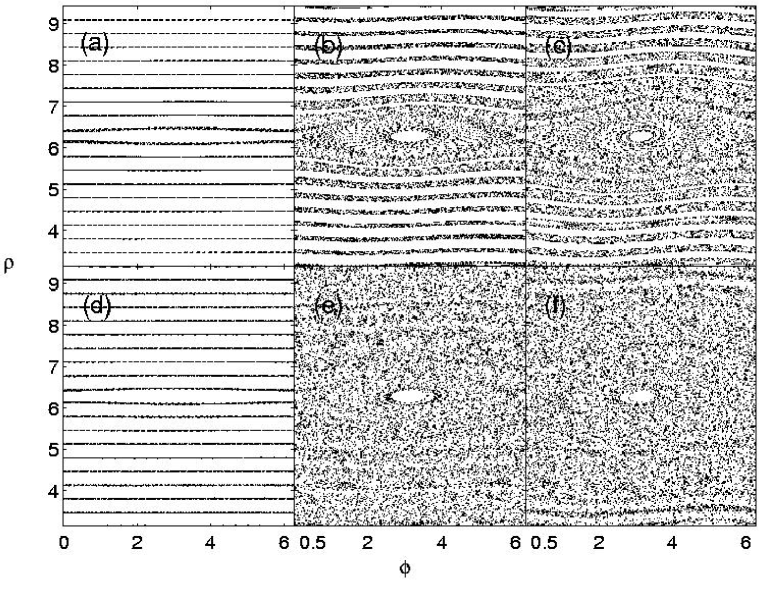
Figure 4: Phase space portraits for the $\epsilon$–classical standard map for $\mathchar 22\relax\mkern-9.0muk=2\pi$ and $k=3.7$. The figures in the first row ((a), (b) and (c)) are for an amplitude noise level of $0$ and for values of $\epsilon$ of $0.001$,$0.02$ and $0.04$ respectively. The second row (figures (d), (e) and (f)) show the $\epsilon$–classical phase space for an amplitude noise level of $2$ and the same values of $\epsilon$. In Fig. 3(b), the values of $\mathchar 22\relax\mkern-9.0muk$ corresponding to $\epsilon=0.001$, $0.02$ and $0.04$ are labelled A,B and C respectively.

The formula for the early time energy growth rate $D$ also provides us with predictions of the qualitative behaviour of the late time energy Auckland2003 . However, if we limit our attention to the energies for $\mathchar 22\relax\mkern-9.0muk\approx 2\pi m$ where $m$ is a positive integer, the $\epsilon$–classical model of Wimberger et al. may be employed to calculate the energies around the quantum resonance after larger numbers of kicks. If $\epsilon=2\pi m-\mathchar 22\relax\mkern-9.0muk$ is the (small) difference between $\mathchar 22\relax\mkern-9.0muk$ and a resonant point, the dynamics of the AOKR is well approximated by the map Wimberger2003

$$\rho_{n+1} = \rho_{n}+\tilde{k}_{n}\sin\phi_{n+1},$$ (12a)

$$\phi_{n+1} = \phi_{n}+{\rm{sign}}(\epsilon)\rho_{n}+\pi l+\mathchar 22\relax\mkern-9.0muk\beta\mod 2\pi,$$ (12b)

where $\tilde{k_{n}}=|\epsilon|k_{n}$, $k_{n}=(\kappa/\mathchar 22\relax\mkern-9.0muk)R_{A,n}$ Schlunk2003a , $\rho_{n}$ and $\phi_{n}$ are the momentum and position at kick $n$ respectively, $\rho_{0}=|\epsilon|n_{0}$ for $n_{0}$ a positive integer and $\epsilon=\mathchar 22\relax\mkern-9.0muk-2\pi m\ll 1$ for positive integers $m$. In this paper, $l$ is set to $1$ without loss of generality as in references Wimberger2003 ; Wimberger2003bpp . In the reformulated dynamics, $\epsilon$ plays the part of Planck’s constant and $\epsilon\rightarrow 0$ may be considered to be a quasi–classical limit.

Fig. 3(b) shows the energy peak produced by the $\epsilon$–classical dynamics for various amplitude noise levels. We see that even the maximum noise level of $2$ does not destroy the peak, a finding that agrees with the experimental and simulation results presented in the previous section. Wimberger et al. have derived a scaling law for the ratio of the mean energy at a certain value of $\epsilon$ to the on–resonant energy. This ratio is a function of $\epsilon$, the kicking strength $\kappa/\mathchar 22\relax\mkern-9.0muk$ and the kick number Wimberger2003 ; Wimberger2003bpp . The scaling law reproduces the quantum resonance peak, and its form is found to arise from the changes in the $\epsilon$–classical phase space as $\epsilon$ is varied and $\kappa/\mathchar 22\relax\mkern-9.0muk$ is held constant. These changes may be seen in Fig. 4. The first row shows the $\epsilon$–classical phase space for increasing $\epsilon$ and no amplitude noise. For the relatively unperturbed system which exists at very low values of $\epsilon$ (say $\epsilon<0.001$), lines of constant momentum dominate the phase space (see Fig. 4(a)).

We now consider the near resonant mechanics when zero noise is present, so that $k_{n}=k={\rm constant}$ for all $n$. In this case, following Wimberger et al., we may calculate the kinetic energy $E_{n}=\epsilon^{-2}\langle\rho_{n}^{2}/2\rangle$ by neglecting terms of order $\epsilon$ in Eq. (12b) and iterating Eqs. (12)(a) and (b) followed by averaging over $\phi_{0}$ and $\beta$. Iterating Eq. (12) in the limit of vanishing $\epsilon$, and considering for simplicity only the case where $\epsilon>0$ and $\rho_{0}=0$, we find the momentum after the $n$th kick to be Wimberger2003bpp

$$\rho_{n}\approx\epsilon k\sum_{s=0}^{n-1}\sin(\phi_{0}+\pi(1+2\beta)s),$$ (13)

whence the mean energy may be calculated as

$$E_{n}\approx\frac{k^{2}}{2}\left\langle\sum_{s,s^{\prime}=0}^{n-1}\sin(\phi_{0}+\pi(1+2\beta)s)\sin(\phi_{0}+\pi(1+2\beta)s^{\prime})\right\rangle,$$ (14)

where the average on the RHS is taken over all values of $\phi_{0}$.

For $\mathchar 22\relax\mkern-9.0muk=2\pi$ (as in Fig. 4) the resonant value of quasi–momentum is $\beta=0.5$ dArcy2003pp (corresponding to the line $\rho=2\pi$ in the phase space figures). Substitution of this value of $\beta$ into Eq. (14) followed by averaging over a uniform distribution for $\phi_{0}$ gives $E_{n}\approx(k^{2}/2)n^{2}$ (this expression is exact when $\epsilon=0$) – that is ballistic growth of energy occurs at exact quantum resonance for $\beta=0.5$ – and the mean energy of the atomic ensemble (i.e. averaging over $\beta$) is raised significantly as $\epsilon\rightarrow 0$ (in fact it grows linearly with kick number Wimberger2003bpp ). Thus, the uniquely quantum energy peak found at integer multiples of $\mathchar 22\relax\mkern-9.0muk=2\pi$ may also be explained by a classical resonance of the $\epsilon$–classical dynamics which is valid in this regime.

For larger values of $\epsilon$, the phase space of the system is significantly distorted and the approximate expression in Eq.(13) is no longer valid. However, two facts in particular give a qualitative explanation for the decline in mean energy away from exact resonance: Firstly, the most distorted area of phase space is that around $\rho=2\pi$ – that is the region responsible for ballistic growth for vanishing $\epsilon$ Wimberger2003 . Thus the number of trajectories giving ballistic growth is drastically lessened for $\epsilon>0$. Secondly, although the phase space region responsible for ballistic energy growth is warped, the structures which prevent stochastic energy growth (KAM tori) remain for $\epsilon>0$ and so the full quasi–linear rate of energy growth is not attained. These two facts taken together give a qualitative explanation for the fall off in mean energy as $\epsilon$ is increased, as seen in Fig. 3(b).

This qualitative explanation of the structure near quantum resonance also holds in the case where maximal amplitude noise is applied to the system, as seen in the second row of Fig. 4. At exact quantum resonance ($\epsilon=0$) ballistic motion still occurs even in the presence of amplitude noise. For $\epsilon>0$, the phase space is distorted as before and some invariant curves are destroyed by the applied noise. However, even for $\epsilon=0.04$ (Fig. 4(f)), the phase space has not become completely stochastic and so we see the same quantum resonance structure as in the no–noise case, albeit with a lower peak–to–valley energy ratio.

The persistence of the quantum resonance structure in the presence of amplitude noise may now be seen to be due to the reappearance of the quasi–classical dynamics which occurs at values of $\mathchar 22\relax\mkern-9.0muk$ close to resonance value, and far from the actual classical limit. The $\epsilon$–classical description which is valid in this regime is marked by a return to complete integrability exactly at quantum resonance. By contrast, the extreme sensitivity of the resonant peak to even small amounts of period noise is precisely due to the sensitivity of this approximation to the exact value of $\mathchar 22\relax\mkern-9.0muk$ (and thus the pulse timing). Whilst similar arguments to those used for amplitude noise might suggest that the resonance peak should be robust to period noise too, it is the very reappearance of the stable dynamics which is actually ruined by this type of noise. If the mean deviation from periodicity is of the order of the width of the quantum resonance peak, the suppression of energy growth to either side of the peak is destroyed, and the final energy approaches the zero correlation limit for any value of the kicking period. Comparison with the resonance seen in the early energy growth rates in the actual classical limit (Fig. 3(a)) shows that the behaviour of the quantum resonance in the presence of amplitude noise is qualitatively identical to that of the classical resonance. Thus, although the $\epsilon$–classical description of quantum resonance employs a “fictitious” classical dynamics in which the effective Planck’s constant is still far from $0$, the quantum resonance peak may be said to mark a reappearance of classical stability in the kicked rotor dynamics far from the classical limit. The experimental observation of the robustness of the quantum resonance peak provides a new test of the validity of the $\epsilon$–classical model for the AOKR.

VII Conclusion

We have presented experimental results demonstrating that the quantum resonance peaks observed in Atom Optics Kicked Rotor experiments are surprisingly robust to noise applied to the kicking amplitude, and that quantum resonance peaks are still experimentally detectable even at the maximum possible noise level. By contrast the application of even small amounts of noise to the kicking period is sufficient to completely destroy the resonant peak and return the behaviour of the system to the zero–correlation limit. We have shown that the stability of the resonant dynamics in the presence of amplitude noise is reproduced by the $\epsilon$–classical dynamics of Wimberger et al. Viewed in light of this theoretical treatment, the resilience of the quantum resonance peak to amplitude noise is due to the reappearance of near–integrable $\epsilon$–classical dynamics near quantum resonance, the behaviour of which is analogous (although not identical) to that of the kicked rotor in the actual classical limit of $\mathchar 22\relax\mkern-9.0muk\rightarrow 0$.

References

- (1) See, for example, W.H. Zurek and J.P. Paz, Phys. Rev. Lett. 72 2508 (1994), E. Ott and T.M. Antonsen, Jr, and J.D. Hanson Phys. Rev. Lett. 53 2187 (1984), W.H. Zurek Physics Today 44, 36 (1991).
- (2) F.L. Moore, J.C. Robinson, C.F. Bharucha, B. Sundaram, and M.G. Raizen Phys. Rev. Lett. 75 4598 (1995).
- (3) M.G. Raizen, F.L. Moore J.C. Robinson, C.F. Bharucha, and B. Sundaram Quant. & Semiclass. Optics 8 687-92 (1996).
- (4) S. Fishman, D.R. Grempel, and R.E. Prange Phys. Rev. Lett. 49, 509 (1982)
- (5) F.M. Izrailev and D.L. Shepelyansky Sov. Phys. Dokl. 24, 996 (1979)
- (6) H. Ammann, R. Gray, I. Shvarchuck and N. Christensen Phys. Rev. Lett. 80 4111 (1998).
- (7) B.G. Klappauf, W.H. Oskay, D.A. Steck and M.G. Raizen Phys. Rev. Lett. 81 1203 (1998).
- (8) M.B. d’Arcy, R.M. Godun, M.K. Oberthaler, D. Cassettari and G.S. Summy Phys. Rev. Lett. 87 074102 (2001).
- (9) M.B. d’Arcy, R.M. Godun, M.K. Oberthaler, G.S. Summy, K. Burnett, and S.A. Gardiner Phys. Rev. E 64 056233 (2001).
- (10) M.B. d’Arcy, R.M. Godun, G.S. Summy, I. Guarneri, S. Wimberger, S. Fishman, and A. Buchleitner, Phys. Rev. E 69, 027201 (2004).
- (11) S. Brouard and J Plata J. Phys. A 36 3745 (2003).
- (12) S. Schlunk, M.B. d’Arcy, S. A. Gardiner, D. Cassettari, R.M. Godun, and G.S. Summy, Phys. Rev. Lett. 90 054101 (2003)
- (13) S. Schlunk, M.B. d’Arcy, S.A. Gardiner, and G.S. Summy Phys. Rev. Lett. 90 124102 (2003)
- (14) M.E.K. Williams, M.P. Sadgrove, A.J. Daley, R.N.C. Gray, S.M. Tan, A.S. Parkins, R. Leonhardt, and N. Christensen, J. Opt. B 6 28 (2004).
- (15) W.H. Oskay, D.A. Steck, M.G. Raizen, Chaos, Solitons and Fractals, 16, 409 (2003).
- (16) W.H. Oskay, D.A. Steck, V. Milner, B.G. Klappauf, and M.G. Raizen Opt. Comm. 179 137 (2000).
- (17) L. Deng, E.W. Hagley, J.Denschlag, J.E. Simsarian, Mark Edwards, Charles W. Clark, K. Helmerson, S.L. Rolston and W.D. Phillips Phys. Rev. Lett. 83 5407 (1999)
- (18) S. Wimberger, I. Guarneri, and S. Fishman, Nonlin. 16 1381 (2003).
- (19) C. Monroe, W. Swann, H. Robinson and C. Wieman, Phys. Rev. Lett., 65, 1571 (1990)
- (20) FSMLabs Inc., http://www.fsmlabs.com/products/rtlinuxpro/rtlinuxpro_faq.html.
- (21) A.J. Daley, A.S. Parkins, R. Leonhardt, and S.M. Tan, Phys. Rev. E, 65, 035201 (2002).
- (22) R. Graham, M. Schlautmann and P. Zoller, Phys. Rev. A, 45, R19 (1992)
- (23) S. Wimberger, I. Guarneri, and S. Fishman, Nonlin. 16 1381 (2003).
- (24) D.A. Steck, V. Milner, Windell H. Oskay, and M.G. Raizen Phys. Rev. E 62 3461 (2000).
- (25) A.B. Rechester and R.B. White, Phys. Rev. Lett. 44 1586 (1980)
- (26) H.J. Metcalf and P. van der Straten, Springer, (1999)
- (27) M.P. Sadgrove, Masters Thesis, University of Auckland.
- (28) S. Wimberger, I. Guarneri, and S. Fishman, Phys. Rev. Lett. 92,084102 (2004).
- (29) D.L. Shepelyansky, Physica D 28, 103 (1987).
- (30) A.J. Daley and A.S. Parkins, Phys. Rev. E, 66, 056210 (2002)