Abstract

The original Wigner function provides a way of representing in phase space the quantum states of systems with continuous degrees of freedom. Wigner functions have also been developed for discrete quantum systems, one popular version being defined on a $2N\times 2N$ discrete phase space for a system with $N$ orthogonal states. Here we investigate an alternative class of discrete Wigner functions, in which the field of real numbers that labels the axes of continuous phase space is replaced by a finite field having $N$ elements. There exists such a field if and only if $N$ is a power of a prime; so our formulation can be applied directly only to systems for which the state-space dimension takes such a value. Though this condition may seem limiting, we note that any quantum computer based on qubits meets the condition and can thus be accommodated within our scheme. The geometry of our $N\times N$ phase space also leads naturally to a method of constructing a complete set of $N+1$ mutually unbiased bases for the state space.

PACS numbers: 03.65.Ta, 02.10.-v

1 Introduction

Given any pure or mixed state of a quantum system with continuous degrees of freedom, one can represent the state by its Wigner function [1, 2], a real function on phase space. The Wigner function acts in some respects like a probability distribution, but it differs from a probability distribution in that it can take negative values. The Wigner function has been widely used in semiclassical calculations, and it is also used to facilitate the visualization and tomographic reconstruction of quantum states. For a system with a single degree of freedom, one of the most interesting features of the Wigner function is this: if one integrates the function along any axis in the two-dimensional phase space—the axis can represent any linear combination of position and momentum—the result is the correct probability distribution for an observable associated with that axis [3, 4].

Generalizations of the Wigner function have been proposed that apply to quantum systems with a finite number $N$ of orthogonal states, and the present paper continues this line of research. In 1974 Buot introduced a discrete Weyl transform which, when applied to a one-dimensional periodic lattice of $N$ sites (with $N$ odd), generates a Wigner function defined on a phase space consisting of an $N\times N$ array of points [5]. Buot’s work is related to earlier work by Schwinger [6], who did not explicitly generalize the Wigner function but identified a complete basis of $N^{2}$ orthogonal unitary operators (elements of the generalized Pauli group—or discrete Weyl-Heisenberg group) that can be used to define an $N\times N$ phase space. A different approach was taken in 1980 by Hannay and Berry [7]: these authors directly adapted the definition of the continuous Wigner function to a periodic lattice and thereby arrived at a discrete Wigner function defined on a $2N\times 2N$ phase space.

Both of these basic approaches were later rediscovered and developed further by other researchers. Variations on the $N\times N$ scheme were proposed by Wootters [4], Galetti and De Toledo Piza [8], and Cohendet et al. [9], following initial investigations into the $N=2$ case by Cohen and Scully [10] and Feynman [11]. The $N\times N$ phase-space description has been applied to quantum optics by Vaccaro and Pegg [15] and to quantum teleportation by Koniorczyk et al. [16]. Discrete Wigner functions on the $2N\times 2N$ model have been investigated by Leonhardt [14] and used by Bianucci et al., Miquel et al., and Paz to analyze various quantum processes such as the Grover search algorithm [17]. All of these proposals have the feature that one can sum the Wigner function along different axes in the discrete phase space (including skew axes) to obtain correct probability distributions for observables associated with those axes. Leonhardt in particular has emphasized the value of this feature for tomography, that is, for ascertaining the quantum state of a given ensemble by performing a series of measurements on subensembles. Other discrete Wigner functions have been considered which do not have this feature [18], but in the work we present here this tomographic property plays a central role. One can find further discussion of discrete Wigner functions and their history in, for example, Refs. [12, 13, 53].

In the continuous case, for a system with one degree of freedom, one can regard the Wigner function as being based on a certain quantum structure that one imposes on the classical phase space. The structure consists of assigning to each straight line in phase space a particular quantum state. Let $q$ and $p$ be the phase-space coordinates, and suppose that the line in question is the solution to the linear equation $aq+bp=c$. Then the quantum state assigned to this line is the eigenstate of the operator $a\hat{q}+b\hat{p}$ with eigenvalue $c$. Once this connection is made between lines in phase space and quantum states, one defines the Wigner function as $W(q,p)=(1/2\pi\hbar)\,\hbox{Tr}\,[\rho A(q,p)]$, where $\rho$ is the density matrix being represented and the operator $A(q,p)$ is built in a symmetric way out of all the quantum states assigned to lines of phase space, the weight given to a particular state depending on the relationship of its line to the point $(q,p)$.

In this paper we wish to define a discrete Wigner function—actually a class of discrete Wigner functions—following as closely as possible the spirit of the construction just described. Because this construction is essentially geometrical, we want the geometry of our discrete phase space to be closely analogous to the geometry of an ordinary plane. For example, we need to have the concept of “parallel lines” in phase space, and we want two non-parallel lines always to intersect in exactly one point, just as in the Euclidean plane. Such considerations lead us to use, as the variables that label the axes of phase space, quantities that take values in a field in the algebraic sense. That is, for our axis variables $q$ and $p$, we replace the usual real coordinates with coordinates taking values in $\mathbb{F}_{N}$, the finite field with $N$ elements. (Our phase space can therefore be pictured as an $N\times N$ lattice.) Now, there exists a field having exactly $N$ elements if and only if $N$ is a power of a prime [19]. Thus our formulation is directly applicable only to quantum systems for which the dimension of the state space is such a number. It is always possible to extend it to other values of $N$ by taking Cartesian products of the basic phase spaces—the same strategy is used in Ref. [4], and indeed, exactly the same strategy is used in the continuous case when there is more than one degree of freedom—but in this paper we will restrict our attention to the basic phase spaces with field elements as coordinates. The use of arbitrary finite fields is what distinguishes our work from earlier approaches to discrete phase space.

Though the restriction to powers of primes rules out many quantum systems, there is one familiar case to which our formulation may be ideally suited, namely, a system of $n$ qubits such as is commonly used to model a quantum computer. In that case the dimension of the state space is $N=2^{n}$, which is indeed a power of a prime. Thus our version of the discrete Wigner function provides an alternative to the $2N\times 2N$ formulation that has been most frequently used in quantum information theoretic applications. Most likely each of these phase-space formulations will prove to have its own advantages.

As in the continuous case, we impose a quantum structure on the $N\times N$ phase space by assigning a quantum state to each line in phase space. We insist that this assignment satisfy a certain strong constraint, namely, that it transform in a particular way under translations. (The analogous quantum structure on the continuous phase space satisfies a similar constraint.) Any assignment of quantum states to lines that meets this condition we call a “quantum net,” and we use it to define a discrete Wigner function. It turns out that the requirement of translational covariance does not pick out a unique assignment of quantum states to phase-space lines; that is, there is not a unique quantum net for a given $N\times N$ phase space. Moreover, we have not found a general principle that would select, in a natural way, one particular quantum net for each $N$. So our approach does not lead immediately to a unique Wigner function for a quantum system with $N$ orthogonal states. To some extent this non-uniqueness is mitigated by the fact that many different quantum nets are closely related to each other. We define notions of “equivalence” and “similarity” for quantum nets and identify the similarity classes for $N=2$, 3, and 4. A good portion of the paper is devoted to this classification of quantum nets, which amounts to a classification of possible definitions of the Wigner function within this framework.

One motivation for the present work comes from quantum tomography, which we mentioned above in connection with other discrete versions of the Wigner function as well as the continuous version. As we will see, our approach leads naturally to a specific tomographic technique. Each complete set of parallel lines in the discrete phase space corresponds to a particular measurement on the quantum system, or more precisely, to a particular orthogonal basis for the state space. By experimentally determining the probabilities of the outcomes of this measurement, one can obtain some information about the Wigner function, namely, the sum of the Wigner function over each of those parallel lines. The sums over all the lines of phase space are sufficient to reconstruct the entire Wigner function and thus determine the state of the system.

The particular orthogonal bases that are associated with sets of parallel lines turn out to be mutually unbiased, or mutually conjugate; that is, each vector in one of these bases is an equal-magnitude superposition of all the vectors in any of the other bases. Sets of mutually unbiased bases have been used before, not only for state determination [20, 21] but also for quantum cryptography and in other contexts [22, 29], and a few methods have been found for generating such bases [23, 24, 20, 25, 26, 27, 28, 29, 30]. As we will see, the discrete phase space developed in this paper leads to a rather elegant way of constructing mutually unbiased bases; it is essentially the same method as was discovered recently by Pittenger and Rubin [28] and is closely related to the recent work of Durt [29], though those authors were not studying phase space or Wigner functions. The connection with mutually unbiased bases—valid for all prime power dimensions $N$—is one respect in which the Wigner function presented here is different from those proposed earlier. A consequence is that the tomographic scheme suggested by our phase space construction involves fewer distinct measurements than schemes derived from other discrete phase spaces [20, 21]. This feature is the focus of Ref. [31], which introduces for certain special cases some of the ideas that we present here in a more general setting.

As further motivation, we note that the discrete Wigner function we develop here appears to bear an interesting relation to certain toy models of quantum mechanics proposed by Hardy [32] and Spekkens [33] to address foundational issues. For example, in both of these models a “toybit” has exactly four underlying ontic states, which could be taken to correspond to the four points of our one-qubit phase space. As has been suggested by Spekkens, the discrete Wigner function might therefore facilitate the comparison between quantum mechanics and these toy theories [33].

Our discrete phase space is also related to some work on quantum error correcting codes, which is similarly based on finite fields. (In Section 4 we point out aspects of this relationship.) It is conceivable, then, that our Wigner function could be of particular value when representing certain encodings of quantum states.

The remaining sections are organized as follows. Section 2 recalls the definition of the usual Wigner function and shows how it can be obtained from an assignment of quantum states to the lines of phase space. In Section 3 we give the mathematical description of our discrete phase space and discuss its geometrical properties. Section 4 shows how to build a quantum net on this discrete phase space and shows that the bases associated with different sets of parallel lines must be mutually unbiased. The notion of a quantum net is then used in Section 5 to construct a discrete Wigner function. In Sections 6 and 7 we define our notions of equivalence and similarity between quantum nets and identify the similarity classes for small values of $N$. Finally in Section 8 we review our results and contrast the discrete and continuous cases.

2 The Wigner function constructed from eigenstates of $a\hat{q}+b\hat{p}$

Here we briefly derive the usual definition of the continuous Wigner function in a way that lends itself to generalization to the discrete case. The quantum system in question is a particle moving in one dimension, and the coordinates of phase space are the position $q$ and momentum $p$.

We begin by assigning a quantum state to each line in phase space. Consider the line specified by the equation $aq+bp=c$, where the real numbers $a$, $b$, and $c$ are arbitrary except that $a$ and $b$ cannot both be zero. To this line we assign the unique eigenstate of the operator $a\hat{q}+b\hat{p}$ that has eigenvalue $c$. In the position representation we can write this operator as

$$a\hat{q}+b\hat{p}=aq-ib\hbar\frac{d}{dq}\,,$$ (1)

and the relevant eigenstate $|\psi_{abc}\rangle$ is given by

$$\langle q|\psi_{abc}\rangle=\psi_{abc}(q)=\frac{1}{\sqrt{2\pi\hbar|b|}}e^{-i(a/2\hbar b)(q-c/a)^{2}}.$$ (2)

The normalization of $\psi_{abc}$ is chosen so that the integral $\int_{c_{1}}^{c_{2}}|\psi_{abc}\rangle\langle\psi_{abc}|dc$, with $c_{2}>c_{1}$, is a projection operator.

As we mentioned in the Introduction, given a density matrix $\rho$ of the particle, the corresponding Wigner function will be of the form

$$W(q,p)=\frac{1}{2\pi\hbar}\,\hbox{Tr}\,[\rho A(q,p)],$$ (3)

where $A(q,p)$ is an operator that we will assign to the point $(q,p)$. This operator is constructed, as we will see below, out of the states $|\psi_{abc}\rangle$.

We want the Wigner function to have the property that its integral over the strip of phase space bounded by the lines $aq+bp=c_{1}$ and $aq+bp=c_{2}$ is the probability that the operator $a\hat{q}+b\hat{p}$ will take a value between $c_{1}$ and $c_{2}$. This is one of the characteristic features of the Wigner function and is the property that makes it so useful for tomography. We can guarantee this property by insisting that the integral of $(1/2\pi\hbar)A(q,p)$ over the same strip of phase space is the projection operator onto the subspace corresponding to the eigenvalues of $a\hat{q}+b\hat{p}$ lying between $c_{1}$ and $c_{2}$. That is, we insist that

$$\frac{1}{2\pi\hbar}\int_{\hbox{{\scriptsize strip}}}A(q,p)\,dq\,dp=\int_{c_{1}}^{c_{2}}|\psi_{abc}\rangle\langle\psi_{abc}|\,dc,\;\hbox{for}\;c_{2}>c_{1}.$$ (4)

An equivalent expression of this condition, in terms of a single line in phase space rather than a strip, is the following:

$$\frac{1}{2\pi\hbar}\int\delta(c-aq-bp)A(q,p)\,dq\,dp=|\psi_{abc}\rangle\langle\psi_{abc}|.$$ (5)

To find $A(q,p)$ explicitly, we need to invert Eq. (5). But Eq. (5) is an example of the well-studied Radon transform—the operator $|\psi_{abc}\rangle\langle\psi_{abc}|$, regarded as a function of $a$, $b$, and $c$, is the Radon transform of $(1/2\pi\hbar)A(q,p)$ regarded as a function of $q$ and $p$—and the inverse of this transform is well known [34]. Here we simply state the result:

$$A(q,p)=-\frac{\hbar|c|}{\pi}\int_{-\infty}^{\infty}\int_{-\infty}^{\infty}\left({\mathcal{R}}\frac{1}{(c-aq-bp)^{2}}\right)|\psi_{abc}\rangle\langle\psi_{abc}|\,da\,db\,,$$ (6)

where $c$ is any nonzero real constant, and ${\mathcal{R}}$ indicates the canonical regularization of the singular function that follows it. In the case of the function $1/x^{2}$, this regularization is defined by

$$\int_{-\infty}^{\infty}\left({\mathcal{R}}\frac{1}{x^{2}}\right)f(x)\,dx=\int_{0}^{\infty}\frac{f(x)+f(-x)-2f(0)}{x^{2}}\,dx.$$ (7)

Using the expression for $\psi_{abc}$ of Eq. (2), one can carry out the integration of Eq. (6) to get

$$\langle q^{\prime}|A(q,p)|q^{\prime\prime}\rangle=\delta\left(\frac{q^{\prime}+q^{\prime\prime}}{2}-q\right)e^{(ip/\hbar)(q^{\prime}-q^{\prime\prime})}.$$ (8)

The Wigner function then comes out to be

$$W(q,p)=\frac{1}{2\pi\hbar}\hbox{Tr}\,[\rho A(q,p)]=\frac{1}{\pi\hbar}\int_{-\infty}^{\infty}\langle q-x|\rho|q+x\rangle e^{2ixp/\hbar}\,dx.$$ (9)

Notice that according to the inverse Radon transform given in Eq. (6), the operator $A(q,p)$ is built out of all the operators $|\psi_{abc}\rangle\langle\psi_{abc}|$, the weight given to each operator tending to fall off as the associated line gets farther from the point $(q,p)$. We will find that the analogous inversion in the discrete phase space is much simpler: the $A$ operator associated with a given point is built entirely from the states assigned to the lines passing through that point.

A particular property of the Wigner function that we want to generalize to the discrete case is translational covariance [2]. Here we state the property without proof. Let $W(q,p)$ be the Wigner function corresponding to a density matrix $\rho$, and let $\rho^{\prime}$ be obtained from $\rho$ by a displacement $x$ in position and a boost $y$ in momentum:

$$\rho^{\prime}=e^{i(y\hat{q}-x\hat{p})/\hbar}\rho e^{-i(y\hat{q}-x\hat{p})/\hbar}.$$ (10)

Then the Wigner function $W^{\prime}$ corresponding to $\rho^{\prime}$ is obtained from $W$ via the transformation

$$W^{\prime}(q,p)=W(q-x,p-y).$$ (11)

That is, when the density matrix is translated, the Wigner function follows along rigidly.

Before moving on to the discrete phase space, let us mention an interesting property of the states $|\psi_{abc}\rangle$ that likewise has an analogue in the discrete case. Consider two infinite strips $S$ and $S^{\prime}$ of phase space that are not parallel. The strip $S$ is bounded by the lines $aq+bp=c_{1}$ and $aq+bp=c_{2}$, while $S^{\prime}$ is bounded by $a^{\prime}q+b^{\prime}p=c_{1}^{\prime}$ and $a^{\prime}q+b^{\prime}p=c_{2}^{\prime}$, and we assume that $c_{2}>c_{1}$ and $c_{2}^{\prime}>c_{1}^{\prime}$. Let $P$ be the projection operator onto the subspace associated with $S$; i.e.,

$$P=\int_{c_{1}}^{c_{2}}|\psi_{abc}\rangle\langle\psi_{abc}|dc.$$ (12)

Similarly, let $P^{\prime}$ be the projection onto the subspace associated with $S^{\prime}$. Using Eq. (2) we can write down an explicit expression for $P$ in the position representation (with a suitable modification if $b=0$):

$$\langle q|P|q^{\prime}\rangle=\frac{1}{\pi(q-q^{\prime})}\sin\left[\frac{(c_{2}-c_{1})(q-q^{\prime})}{2\hbar|b|}\right]e^{-(i/2\hbar b)(q-q^{\prime})[a(q+q^{\prime})-(c_{1}+c_{2})]}$$ (13)

and $P^{\prime}$ can be written similarly. One can show by explicit integration that the quantity Tr($PP^{\prime}$), that is, $\int\langle q|P|q^{\prime}\rangle\langle q^{\prime}|P^{\prime}|q\rangle\,dq\,dq^{\prime}$, works out to be

$$\hbox{Tr}\,(PP^{\prime})=\frac{1}{2\pi\hbar}\,\frac{(c_{2}-c_{1})(c_{2}^{\prime}-c_{1}^{\prime})}{|ab^{\prime}-a^{\prime}b|}.$$ (14)

But the positive quantity $(c_{2}-c_{1})(c_{2}^{\prime}-c_{1}^{\prime})/|ab^{\prime}-a^{\prime}b|$ is simply the area of the region where the two infinite strips overlap. Thus Tr($PP^{\prime}$) is equal to this area expressed in units of Planck’s constant. In the limit as the width of the strip $S$ shrinks to zero, this result tells us that any eigenstate of the operator $a\hat{q}+b\hat{p}$ yields a uniform distribution of the values of the operator $a^{\prime}\hat{q}+b^{\prime}\hat{p}$.

As we will see, the analogue of this property in the case of discrete phase space is simpler. In place of strips we will consider individual lines of the discrete phase space. As we have said in the Introduction, each complete set of parallel lines will be associated with an orthogonal basis, and one finds that the magnitude of the inner product between any two vectors chosen from different bases is always the same. This is the property called mutual unbiasedness. Before we can see how this comes about, and before we explore discrete generalizations of the Wigner function, we need to define our discrete phase space.

3 Mathematical description of discrete phase space

Our approach to generalizing the continuous phase space to the discrete case is quite simple. Like the continuous phase space for a system with one degree of freedom, our discrete phase space is a two-dimensional vector space, with points labeled by the ordered pair $(q,p)$. But instead of being a vector space over the real numbers, it is a vector space over a finite field, and $q$ and $p$ are field elements. The number of elements in the finite field is the dimension $N$ of the state space of the system we are describing. The physical interpretation of this discrete phase space will be left mostly to Section 4. In this section we focus on its mathematical properties.

A field, in the algebraic sense, is an arithmetic system with addition and multiplication, such that the operations are commutative, associative, distributive, and invertible (except that there is no multiplicative inverse for the number zero) [19]. The real numbers are a familiar example of a field with an infinite number of elements. As we have said in the Introduction, there exists a field with exactly $N$ elements if and only if $N$ is a power of a prime, so our scheme applies directly only to quantum systems for which the state-space dimension is such a number. Moreover for any of these allowed values of $N$, there is essentially only one field having $N$ elements—any two representations are isomorphic—and we label this field ${\mathbb{F}}_{N}$. If $N$ is prime, ${\mathbb{F}}_{N}$ consists of the numbers $0,1,\ldots,N-1$ with addition and multiplication mod $N$. If $N=r^{n}$, with $r$ prime and $n$ an integer greater than 1, then the field ${\mathbb{F}}_{N}$ is not modular in this sense but can be constructed from the prime field ${\mathbb{F}}_{r}$; one says that ${\mathbb{F}}_{N}$ is an extension of ${\mathbb{F}}_{r}$.

Let us illustrate this process of extension in the case of ${\mathbb{F}}_{4}$, which we will use frequently as an example. To generate ${\mathbb{F}}_{4}$, one begins by finding a polynomial of degree 2, with coefficients in ${\mathbb{F}}_{2}$, that cannot be factored in ${\mathbb{F}}_{2}$. (To generate ${\mathbb{F}}_{r^{n}}$ one would use a polynomial of degree $n$.) It happens that the only such polynomial is $x^{2}+x+1$: there is no solution in ${\mathbb{F}}_{2}$ to the equation

$$x^{2}+x+1=0.$$ (15)

The extension is created by introducing a new element $\omega$ that is defined to solve this equation, just as, in creating the complex numbers from the reals, one defines the imaginary element $i$ to solve the equation $x^{2}+1=0$. Once $\omega$ is included, another element, $\omega+1$, is forced into existence, as it were, by the requirement that the field be closed under addition. One thus arrives at ${\mathbb{F}}_{4}$:

$${\mathbb{F}}_{4}=\{0,1,\omega,\omega+1\},$$ (16)

with arithmetic determined uniquely by the fact that $\omega$ satisfies Eq. (15). For example, we can square $\omega$ as follows:

$$\omega^{2}=-\omega-1=(-1)\omega+(-1)=\omega+1,$$ (17)

where we have used the fact that $-1=1$ mod 2. Similarly, we have

$$(\omega+1)^{2}=\omega^{2}+(1+1)\omega+1=\omega^{2}+1=(\omega+1)+1=\omega$$ (18)

Following common practice we will frequently use the symbol $\bar{\omega}$ to represent the field element $\omega+1$. The complete addition and multiplication tables for ${\mathbb{F}}_{4}$ are given here:

+	0	1	$\omega$	$\bar{\omega}$
0	0	1	$\omega$	$\bar{\omega}$
1	1	0	$\bar{\omega}$	$\omega$
$\omega$	$\omega$	$\bar{\omega}$	0	1
$\bar{\omega}$	$\bar{\omega}$	$\omega$	1	0

$\times$	0	1	$\omega$	$\bar{\omega}$
0	0	0	0	0
1	0	1	$\omega$	$\bar{\omega}$
$\omega$	0	$\omega$	$\bar{\omega}$	1
$\bar{\omega}$	0	$\bar{\omega}$	1	$\omega$

We now explore some of the geometric features of the phase space for a generic (but prime power) value of $N$. We picture the space as an $N\times N$ array of points $(q,p)$, with $q$ running along the horizontal axis and $p$ along the vertical axis. For definiteness we place the origin, $(q,p)=(0,0)$, at the lower left-hand corner. The phase space for $N=4$ is shown in Fig. 1(a), and in Fig. 1(b) we show a possible physical interpretation of the axis variables if the space is being used to describe a pair of spin-1/2 particles. (The physical interpretation will be explained further in the following section.) We emphasize, however, that these pictures are not essential to our basic construction. For example, we will often speak of a “vertical line,” but this term is simply shorthand for a set of points of the form $(q,y)$ where $q$ is fixed and $y$ can take any field value.

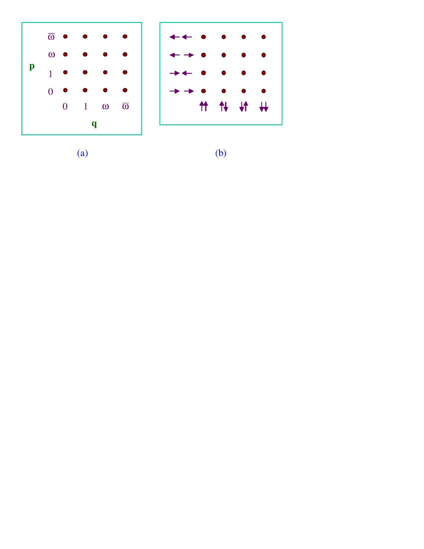
Figure 1: The $4\times 4$ phase space with axes labeled (a) by field elements, and (b) by spin states.

More generally, a line in the $N\times N$ phase space is the set of points satisfying an equation of the form $aq+bp=c$, where $a$, $b$, and $c$ are elements of ${\mathbb{F}}_{N}$ with $a$ and $b$ not both zero. Two lines are parallel if they can be represented by equations having the same $a$ and $b$ but different values of $c$. Because the field operations are so well-behaved—especially since every nonzero element has a multiplicative inverse—the usual rules governing lines and parallel lines apply: (i) given any two distinct points, exactly one line contains both points; (ii) given a point $\alpha$ and a line $\lambda$ not containing $\alpha$, there is exactly one line parallel to $\lambda$ that contains $\alpha$; (iii) two lines that are not parallel intersect in exactly one point. Note that these propositions would not be true for general $N$ if we were always using modular arithmetic, as has been pointed out in Ref. [14]. Consider, for example, the case $N=4$. Under arithmetic mod 4 the points $\{(0,0),(1,2),(2,0),(3,2)\}$ form a line, namely, the line that solves the equation $p=2q$. But $\{(0,0),(1,0),(2,0),(3,0)\}$ is also a line, and it shares two points with the first one.

There are exactly $N(N+1)$ lines in our phase space, and these can be grouped into $N+1$ sets of parallel lines. To see this, note that each nonzero point $(q,p)$ determines a line through the origin, namely, the line consisting of the points $(sq,sp)$ where $s$ takes all values in ${\mathbb{F}}_{N}$. Let us refer to a line through the origin as a ray. Now, there are $N^{2}-1$ nonzero points, but each ray contains $N-1$ such points; so the number of rays is $(N^{2}-1)/(N-1)=N+1$. Each of these rays then defines a set of $N$ parallel lines. Let us call a complete set of parallel lines a “striation” of the phase space. The five striations of the $4\times 4$ phase space are shown in Fig. 2. One can observe there that the lines follow the three rules mentioned above.

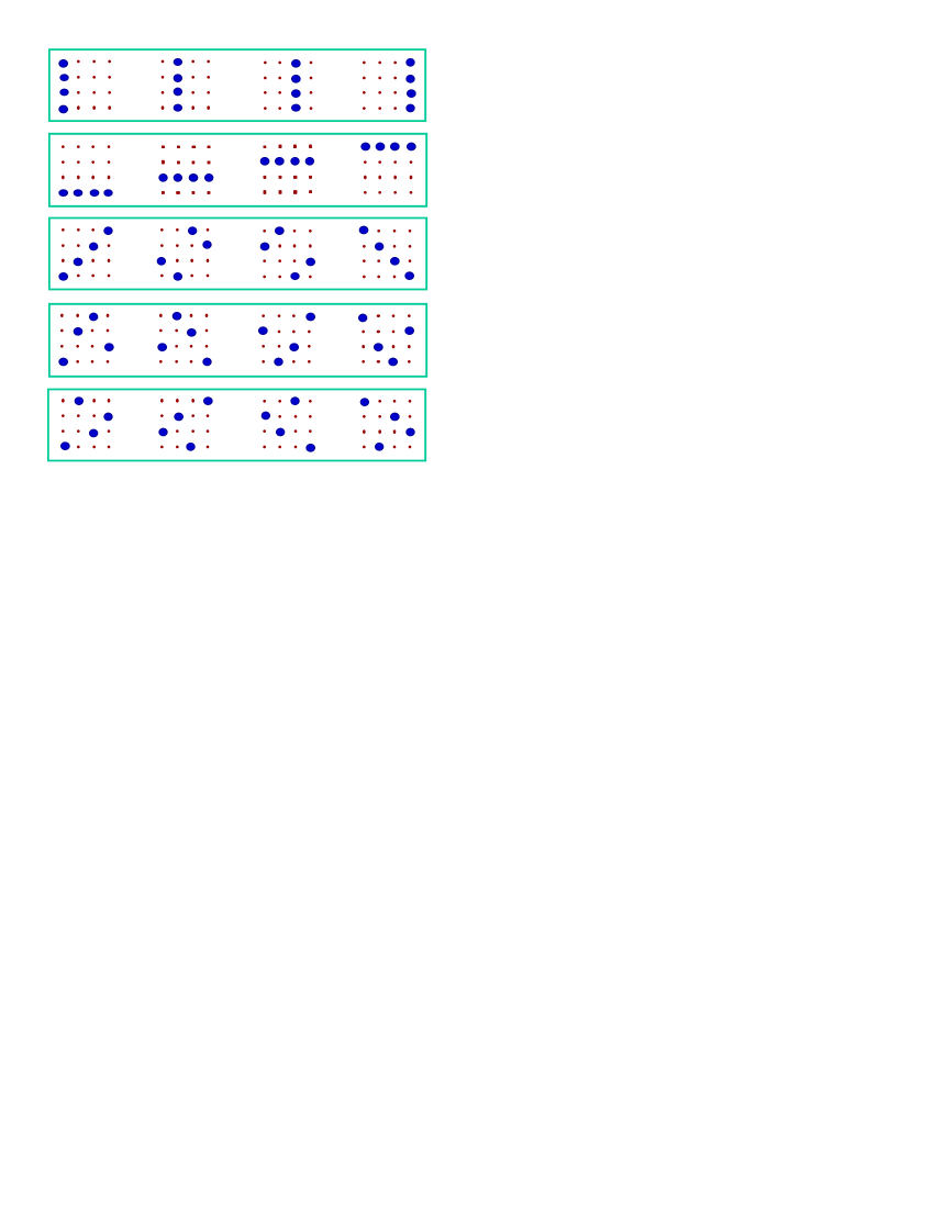
Figure 2: The striations of the $4\times 4$ phase space.

Just as in the continuous case, one can speak of translations of the discrete phase space. A translation is the addition of a constant vector to each point of the space. For example, in the $4\times 4$ phase space as pictured in Fig. 1, translating by the vector $(1,0)$ has the effect of interchanging the first two columns and interchanging the last two columns. We will denote by ${\mathcal{T}}_{\alpha}$ the translation by the vector $\alpha$. ${\mathcal{T}}_{\alpha}$ acts on points in phase space: ${\mathcal{T}}_{\alpha}\beta=\alpha+\beta$. But we will also sometimes apply ${\mathcal{T}}_{\alpha}$ to an entire line, in which case it translates each point in the given line to yield another line (possibly the same as the original).

Shortly we will need the concept of a basis for a field. A basis for the field ${\mathbb{F}}_{r^{n}}$ is an ordered set of field elements $(e_{1},\ldots,e_{n})$ such that every element $x$ in ${\mathbb{F}}_{r^{n}}$ can be expressed in the form

$$x=\sum_{i}^{n}x_{i}e_{i},$$ (19)

where each $x_{i}$ is in the prime field ${\mathbb{F}}_{r}$. There are typically many possible bases for a given field. In ${\mathbb{F}}_{4}$, for example, we could take $(1,\omega)$ as a basis, or $(1,\bar{\omega})$, or $(\omega,\bar{\omega})$. Because in this paper we need to talk about bases for Hilbert spaces as well as bases for fields, we will often refer to the latter as “field bases.”

We will also need the concept of a dual basis, which in turn depends on the notion of the trace of a field element. The trace of a field element $x$ is defined by

$$\hbox{tr}\,x=x+x^{r}+x^{r^{2}}+\cdots+x^{r^{n-1}}.$$ (20)

(We distinguish it from the trace of an operator by the lower case “tr”.) Though this definition may seem quite opaque on first reading, the trace has remarkably simple properties, the most important for us being that (i) the trace is always an element of the prime field ${\mathbb{F}}_{r}$, (ii) $\hbox{tr}\,(x+y)=\hbox{tr}\,x+\hbox{tr}\,y$, and (iii) tr$\,ax=a\,\hbox{tr}\,x$, where $a$ is any element of ${\mathbb{F}}_{r}$. Now, given any basis $E=(e_{1},\ldots,e_{n})$ for ${\mathbb{F}}_{r^{n}}$, there is a unique basis $\tilde{E}=(\tilde{e}_{1},\ldots,\tilde{e}_{n})$ such that

$$\hbox{tr}\,e_{i}\tilde{e}_{j}=\delta_{ij},$$ (21)

where $\delta_{ij}$ is the Kronecker delta. This unique basis is called the dual basis of $E$ [19]. We can immediately use the dual basis to obtain, for fixed basis $E$ and field element $x$, the unique coefficients in the expansion (19). Starting with that expansion, we multiply both sides by $\tilde{e}_{j}$ and take the trace:

$$\hbox{tr}\,(x\tilde{e}_{j})=\sum_{i}^{n}x_{i}\hbox{tr}\,(e_{i}\tilde{e}_{j})=x_{j}.$$ (22)

The expansion coefficients $x_{i}$ will be used in the following section as we lay down a quantum structure on our discrete phase space.

4 Assigning a quantum state to each line in phase space

We now need to supply our discrete phase space with a physical interpretation. We will do this by assigning to each line in phase space a specific pure quantum state as represented by a rank-1 projection operator. Let $Q$ be the function that makes this assignment. That is, for each line $\lambda$ in phase space, $Q(\lambda)$ is the projection operator representing a pure quantum state. We will impose one condition on $Q$, translational covariance, to be defined shortly. A function $Q$ satisfying translational covariance we will call a “quantum net.” Later we will see how each possible choice of the function $Q$ leads to a different definition of the discrete Wigner function.

For $N=r^{n}$ where $r$ is prime, our phase space applies most naturally to a system consisting of $n$ objects (which we call “particles,” though they could be anything), each having an $r$-dimensional state space. We assume that our system has this structure.

We have seen in Eq. (10) the sense in which the continuous Wigner function is translationally covariant. To define an analogous property in the discrete case, we need a discrete analogue of the unitary translation operators

$$T_{(x,y)}=\exp[i(y\hat{q}-x\hat{p})/\hbar]$$ (23)

that appear in Eq. (10). That is, for each discrete phase-space translation ${\mathcal{T}}_{(x,y)}$ with $x$ and $y$ in ${\mathbb{F}}_{N}$, we will define a corresponding unitary operator $T_{(x,y)}$ that acts on the state space. In choosing these unitary operators, we are guided by the following considerations. (i) We want the multiplication of these unitary operators to mimic the composition of translations; that is, we insist that for any vectors $\alpha$ and $\beta$ in phase space,

$$T_{\alpha}T_{\beta}\approx T_{\alpha+\beta},$$ (24)

where the symbol $\approx$ indicates equality up to a phase factor that might depend on $\alpha$ and $\beta$. (The unitary operators of Eq. (23) have exactly the same relation to the addition of continuous phase-space vectors.) (ii) There should be “basic” translations corresponding to unitary operators that act on just one particle. We make the connection between a translation vector $(x,y)$ and individual particles by expanding $x$ and $y$ in field bases, allowing ourselves to use a different basis for each of the two dimensions of phase space. Thus we write

$$x=\sum_{i=1}^{n}x_{ei}e_{i}$$ (25)

and

$$y=\sum_{i=1}^{n}y_{fi}f_{i},$$ (26)

where $E=(e_{1},\ldots,e_{n})$ and $F=(f_{1},\ldots,f_{n})$ are field bases, and we associate the coefficients $x_{ei}$ and $y_{fi}$ with the $i$th particle. (The symbols $e$ and $f$ are included in the subscripts to indicate which basis is being used in the expansion.) A translation that involves only coefficients having a particular value of $i$ should be associated with a unitary operator that acts only on the $i$th particle. (Later we will discuss how much freedom we have in choosing the field bases $E$ and $F$.) (iii) In the single-particle state space, we choose our unitary operators to be as analogous as possible to the continuous operators. Let $(|0\rangle,\ldots,|r-1\rangle)$ be a standard basis for the single-particle state space. Then in the space of the $i$th particle, the “unit horizontal translation,” with $x_{ei}=1$ and $y_{fi}=0$, is associated with the unitary operator $X$ defined by

$$X|k\rangle=|k+1\rangle$$ (27)

with the addition being in ${\mathbb{F}}_{r}$, and the “unit vertical translation,” with $x_{ei}=0$ and $y_{fi}=1$, is assigned the unitary operator $Z$ defined by

$$Z|k\rangle=e^{2\pi ik/r}|k\rangle.$$ (28)

The operators $X$ and $Z$, which are generalized Pauli matrices introduced long ago by Weyl [35], have been used by many authors in many contexts (often with non-prime values of $r$ as in Ref. [36]), including studies of discrete phase spaces [6, 8] and mutually unbiased bases [28, 27]. Except for phase factors, our general unitary translation operators are now fixed by Eqs. (24), (27) and (28). We write them as follows (and this equation fixes the choice of phase factors):

$$T_{(x,y)}=X^{x_{e1}}Z^{y_{f1}}\otimes\cdots\otimes X^{x_{en}}Z^{y_{fn}}.$$ (29)

We note that the operators $T_{(x,y)}$ play an important role in the theory of quantum error correction: they are normally taken as the basic error operators acting on an $r^{n}$-dimensional state space (usually with $r=2$). Often the indices $x_{ei}$ and $y_{fi}$ labeling these error operators are treated simply as elements of ${\mathbb{F}}_{r}$ without the additional field structure that we have assumed. However, for some purposes it has been found useful to treat $x$ and $y$ as elements of the extension ${\mathbb{F}}_{r^{n}}$ as we have done here. (See for example Refs. [37, 38, 39, 40].)

In order for the Wigner function—defined later—to be translationally covariant, we insist that the function $Q(\lambda)$ be translationally covariant in the following sense: for each line $\lambda$ and each phase-space vector $\alpha$,

$$Q({\mathcal{T}}_{\alpha}\lambda)=T_{\alpha}Q(\lambda)T^{\dagger}_{\alpha}.$$ (30)

That is, if we translate a line $\lambda$ in phase space by the vector $\alpha$, the associated quantum state is transformed by $T_{\alpha}$. This is quite a strong requirement. To see why, consider the line consisting of the points $(sx,sy)$ where $x$ and $y$ are fixed (and not both zero) and $s$ ranges over the whole field ${\mathbb{F}}_{N}$. This line, and each of the lines of its striation, are all invariant under a translation by the vector $(sx,sy)$ for any value of $s$. This means that in order to satisfy Eq. (30), the projections $Q$ that we assign to these lines must commute with $T_{(sx,sy)}$ for each value of $s$. (If we were to represent the quantum states by state vectors rather than by projectors, the state vectors assigned to these lines would have to be eigenvectors of $T_{(sx,sy)}$ for each value of $s$.) But this is impossible unless all of the operators $T_{(sx,sy)}$ commute with each other. The basic operators $X$ and $Z$ obey the simple commutation relation

$$ZX=\eta XZ,$$ (31)

where $\eta=e^{2\pi i/r}$. For each value of $s$, the unitary operator $T_{(sx,sy)}$ can be written as

$$T_{(sx,sy)}=X^{(sx)_{e1}}Z^{(sy)_{f1}}\otimes\cdots\otimes X^{(sx)_{en}}Z^{(sy)_{fn}}.$$ (32)

It follows from Eq. (31) that these $N$ operators commute with each other if and only if the following condition is met for all pairs of field elements $s$ and $t$:

$$\sum_{j=1}^{n}(sx)_{ej}(ty)_{fj}=\sum_{j=1}^{n}(tx)_{ej}(sy)_{fj},$$ (33)

where the operations are those of ${\mathbb{F}}_{r}$; that is, they are mod $r$. It turns out that this condition can be very simply expressed in terms of ${\mathbb{F}}_{N}$. We show in Appendix A that Eq. (33) is satisfied for all values of $x$, $y$, $s$ and $t$ if and only if the field bases $E=(e_{1},\ldots,e_{n})$ and $F=(f_{1},\ldots,f_{n})$ are related by an equation of the form

$$f_{i}=w\tilde{e}_{i},\hskip 8.53581pti=1,\ldots,n,$$ (34)

where $w$ is any element of the field ${\mathbb{F}}_{N}$. Thus, because we insist on translational covariance, we are not free to choose the bases $E$ and $F$ arbitrarily. These bases enter into the definitions of the translation operators $T_{\alpha}$, and if the bases do not satisfy Eq. (34), there is no function $Q(\lambda)$ that is translationally covariant with respect to these operators.

Suppose now that $E$ and $F$ do satisfy Eq. (34), so that the $N$ operators $T_{(sx,sy)}$, for fixed $x$ and $y$ and all values of $s$, commute with each other. These unitary operators are traceless and mutually orthogonal in the sense that

$$\hbox{Tr}\,\left(T_{(sx,sy)}^{\dagger}T_{(tx,ty)}\right)=0\hskip 8.53581pt\hbox{if $s\neq t$}.$$ (35)

It follows that they define a unique basis of simultaneous eigenvectors (up to phase factors). Thus as long as this condition on the field bases is satisfied, our requirement of translational covariance picks out a unique orthogonal Hilbert space basis to associate with each striation. (We will see shortly that translational covariance also requires $Q$ to assign a different element of this basis to each line of the given striation.) Moreover, it follows from the work of Bandyopadhyay et al. [27] that these Hilbert space bases are all mutually unbiased. Specifically, Bandyopadhyay et al. show the following: if a set of $N^{2}-1$ traceless and mutually orthogonal $N\times N$ unitary matrices can be partitioned into $N+1$ subsets of equal size, such that the $N-1$ operators in each subset are commuting, then the bases of eigenvectors defined by these subsets are mutually unbiased. Our operators $T_{(x,y)}$ satisfy this hypothesis as long as the field bases $E$ and $F$ satisfy Eq. (34).

Note that because there are $N+1$ striations, the above argument—which again is closely related to Refs. [28] and [29]—shows that one can construct $N+1$ mutually unbiased bases in $N$ complex dimensions when $N$ is a power of a prime. For a general value of $N$ it is known [23, 24] that the number of mutually unbiased bases cannot exceed $N+1$, and other papers have shown in other ways that this number is exactly $N+1$ when $N$ is a power of a prime [20, 25, 26, 27]. Remarkably, the maximum number of such bases appears to be unknown for any value of $N$ that is not a power of a prime (but see Refs. [26, 30, 45, 46, 47] which shed light on that problem).

Let us find the Hilbert space bases that our construction assigns to the vertical and horizontal striations. The vertical lines are invariant under translations by vectors of the form $(0,s)$; so the Hilbert space basis associated with this striation consists of the simultaneous eigenvectors of the operators $T_{(0,s)}$. These operators take the form

$$T_{(0,s)}=Z^{s_{f1}}\otimes\cdots\otimes Z^{s_{fn}}$$ (36)

and are thus all diagonal in the standard basis; so their simultaneous eigenvectors are simply the standard basis vectors

$$|k_{1}\rangle\otimes\cdots\otimes|k_{n}\rangle.$$ (37)

The horizontal lines are invariant under translations by the vectors $(s,0)$; so the Hilbert space basis associated with this striation consists of the simulataneous eigenvectors of

$$T_{(s,0)}=X^{s_{e1}}\otimes\cdots\otimes X^{s_{en}}.$$ (38)

One finds that these vectors are

$$|j_{1})\otimes\cdots\otimes|j_{n}),$$ (39)

where the single-particle states $|j)$, notationally distinguished by the curved bracket, are given by

$$|j)=\frac{1}{\sqrt{r}}\sum_{k=1}^{r}\eta^{jk}|k\rangle.$$ (40)

(Again, $\eta=e^{2\pi i/r}$.) Note that for these two special striations—vertical and horizontal—the associated Hilbert space bases do not depend on the choice of field bases. This is typically not the case for other striations.

Let us see how this all works out for the case $N=4$. First we arbitrarily choose $(e_{1},e_{2})=(\omega,1)$ as the field basis for the horizontal translation variable $x$. One finds that the unique dual of this basis is $(\tilde{e}_{1},\tilde{e}_{2})=(1,\bar{\omega})$. Thus in order to make translational covariance possible we should choose the field basis $(f_{1},f_{2})$ for $y$ to be either $(1,\bar{\omega})$ or some multiple thereof. We achieve a certain simplicity if we multiply $(1,\bar{\omega})$ by $\omega$ to get $(f_{1},f_{2})=(\omega,1)$. Then the basis for $y$ is the same as the basis for $x$. Having made these choices, we can write down the unitary operator associated with any translation. Consider, for example, the following three vectors which are proportional to each other: $(1,\omega),(\omega,\bar{\omega}),(\bar{\omega},1)$. In terms of our field bases, we can express these vectors as $(0e_{1}+1e_{2},1f_{1}+0f_{2}),\;(1e_{1}+0e_{2},1f_{1}+1f_{2}),\;(1e_{1}+1e_{2},0f_{1}+1f_{2}).$ Thus according to Eq. (29) the unitary operators associated with translations by these vectors are, respectively,

$$T_{(1,\omega)}=Z\otimes X,\hskip 14.22636ptT_{(\omega,\bar{\omega})}=XZ\otimes Z,\hskip 14.22636ptT_{(\bar{\omega},1)}=X\otimes XZ,$$ (41)

where in this case $X$ and $Z$ are the ordinary Pauli matrices, expressed in the standard basis as

$$X=\left(\begin{array}[]{cc}0&1\\ 1&0\end{array}\right)\hskip 28.45274ptZ=\left(\begin{array}[]{cc}1&0\\ 0&-1\end{array}\right).$$ (42)

One can verify that the three operators of Eq. (41) commute with each other. The unique basis of simultaneous eigenvectors is

$$\frac{1}{2}\left(\begin{array}[]{c}-1\\ 1\\ i\\ i\end{array}\right)\hskip 8.53581pt\frac{1}{2}\left(\begin{array}[]{c}1\\ -1\\ i\\ i\end{array}\right)\hskip 8.53581pt\frac{1}{2}\left(\begin{array}[]{c}1\\ 1\\ -i\\ i\end{array}\right)\hskip 8.53581pt\frac{1}{2}\left(\begin{array}[]{c}1\\ 1\\ i\\ -i\end{array}\right).$$ (43)

This, then, is the basis that we associate with the striation containing the line $\{(0,0),(1,\omega),(\omega,\bar{\omega}),(\bar{\omega},1)\}$.

In the same way we can figure out what Hilbert space basis is associated with each of the other striations. Fig. 3 shows the complete correspondence explicitly; each striation is labeled, in the left-hand column, by a point belonging to the line in that striation that passes through the origin. The striations are listed in the same order as in Fig. 2. One can verify that these five orthonormal bases are mutually unbiased, as they must be.

(0,1):	$\left(\begin{array}[]{c}1\\ 0\\ 0\\ 0\end{array}\right)$	$\left(\begin{array}[]{c}0\\ 1\\ 0\\ 0\end{array}\right)$	$\left(\begin{array}[]{c}0\\ 0\\ 1\\ 0\end{array}\right)$	$\left(\begin{array}[]{c}0\\ 0\\ 0\\ 1\end{array}\right)$
(1,0):	$\frac{1}{2}\left(\begin{array}[]{c}1\\ 1\\ 1\\ 1\end{array}\right)$	$\frac{1}{2}\left(\begin{array}[]{c}1\\ -1\\ 1\\ -1\end{array}\right)$	$\frac{1}{2}\left(\begin{array}[]{c}1\\ 1\\ -1\\ -1\end{array}\right)$	$\frac{1}{2}\left(\begin{array}[]{c}1\\ -1\\ -1\\ 1\end{array}\right)$
(1,1):	$\frac{1}{2}\left(\begin{array}[]{c}1\\ -i\\ i\\ 1\end{array}\right)$	$\frac{1}{2}\left(\begin{array}[]{c}1\\ i\\ i\\ -1\end{array}\right)$	$\frac{1}{2}\left(\begin{array}[]{c}1\\ -i\\ -i\\ -1\end{array}\right)$	$\frac{1}{2}\left(\begin{array}[]{c}1\\ i\\ -i\\ 1\end{array}\right)$
(1,$\omega$):	$\frac{1}{2}\left(\begin{array}[]{c}1\\ 1\\ i\\ -i\end{array}\right)$	$\frac{1}{2}\left(\begin{array}[]{c}1\\ -1\\ i\\ i\end{array}\right)$	$\frac{1}{2}\left(\begin{array}[]{c}1\\ 1\\ -i\\ i\end{array}\right)$	$\frac{1}{2}\left(\begin{array}[]{c}1\\ -1\\ -i\\ -i\end{array}\right)$
(1,$\bar{\omega}$):	$\frac{1}{2}\left(\begin{array}[]{c}1\\ -i\\ 1\\ i\end{array}\right)$	$\frac{1}{2}\left(\begin{array}[]{c}1\\ i\\ 1\\ -i\end{array}\right)$	$\frac{1}{2}\left(\begin{array}[]{c}1\\ -i\\ -1\\ -i\end{array}\right)$	$\frac{1}{2}\left(\begin{array}[]{c}1\\ i\\ -1\\ i\end{array}\right)$

Figure 3: The five bases generated by the five striations.

So far our construction only assigns a Hilbert-space basis to each striation. Given our definition of $T_{(x,y)}$ in Eq. (29), this assignment is completely determined once we have chosen a field basis for each of the two dimensions of phase space. We now turn to the question of assigning a specific state $Q(\lambda)$ to each line $\lambda$ of phase space. How much freedom do we have in making this assignment?

Consider a striation $S$. Let $B=\{|b_{s}\rangle\}$ be the basis associated with this striation, with $s\in{\mathbb{F}}_{N}$. We now consider a specific line $\lambda_{S0}$ in $S$, namely, the ray that is included in $S$; that is, $\lambda_{S0}$ is the line in $S$ that passes through the origin. We are free to assign any of the states $|b_{s}\rangle$ to $\lambda_{S0}$; this choice is arbitrary. However, once we have made this choice, the vector assigned to any other line of the striation is determined by Eq. (30):

$$Q({\mathcal{T}}_{(x,y)}\lambda_{S0})=T_{(x,y)}Q(\lambda_{S0})T^{\dagger}_{(x,y)},$$ (44)

since any line in the striation can be obtained by translating $\lambda_{S0}$. The function $Q(\lambda)$ is thus entirely determined once we have assigned a quantum state to each of the rays of phase space. Moreover, it is clear from Eq. (44) that the same quantum state cannot be assigned to two distinct lines of a striation: an operator $T_{(x,y)}$ that translates $\lambda$ into $\lambda^{\prime}$ cannot commute with $Q(\lambda)$, since it has a complete set of eigenvectors (not all degenerate) that are unbiased with respect to the basis associated with $\lambda$.

Let us summarize the choices we are allowed as we set up a quantum net for the $N\times N$ phase space. First, we choose a field basis $E$ for the horizontal coordinate; any basis will do. Next, we choose a field basis $F$ for the vertical coordinate, but here we are not so free. $F$ must be a multiple of the unique basis dual to $E$; that is, $f_{i}=w\tilde{e}_{i}$ for some nonzero $w\in{\mathbb{F}}_{N}$. These choices determine the unitary translation operators according to Eq. (29), which in turn define a unique orthonormal basis to be associated with each striation. Now, for each striation $S$, we choose a particular vector $|b\rangle$ in that striation’s basis and let $Q(\lambda_{S0})=|b\rangle\langle b|$, where $\lambda_{S0}$ is the ray defining that striation. The state $Q(\lambda)$ assigned to any other line $\lambda$ is then determined uniquely by the condition $Q({\mathcal{T}}_{(x,y)}\lambda_{S0})=T_{(x,y)}Q(\lambda_{S0})T^{\dagger}_{(x,y)}$.

In the case $N=4$, with the field bases $E=F=(\omega,1)$ as before, we can define a quantum net by choosing, from each of the five bases shown in Fig. 3, one state vector to be associated with the corresponding ray in phase space. For example, we might choose, for each basis, the vector in the left-most column of that table. With this choice, the vertical line through the origin is associated with the state $|00\rangle$ [that is, $k_{1}=k_{2}=0$ in Eq. (37)], and the other vertical lines, from left to right in Fig. 1(a), are associated with the states $|01\rangle$, $|10\rangle$, and $|11\rangle$ respectively. If the system in question is a pair of spin-1/2 particles and if we interpret $|0\rangle$ as $\mid\uparrow\rangle$ and $|1\rangle$ as $\mid\uparrow\rangle$, the vertical lines can be labeled as shown in Fig. 1(b): $\uparrow\uparrow$, $\uparrow\downarrow$, $\downarrow\uparrow$, $\downarrow\downarrow$. With this same choice, the horizontal lines are associated with the states $\mid\rightarrow\rightarrow\rangle$ and so on, as is also indicated in Fig. 1(b).

In the next section we show how we can use a quantum net to define a Wigner function.

5 Defining a Wigner function

A quantum net assigns a state $Q(\lambda)$ to each line $\lambda$ in phase space. The Wigner function $W(q,p)$ of a quantum system should be such that when $W(q,p)$ is summed over the line $\lambda$, the result is the probability that the quantum system will be found in the state $Q(\lambda)$. That is, if $\rho$ is the density matrix of the system, we insist that

$$\sum_{\alpha\in\lambda}W_{\alpha}=\hbox{Tr}\left[\rho Q(\lambda)\right].$$ (45)

For a given quantum net $Q$, this condition completely determines the relation between $\rho$ and $W$.

We now use Eq. (45) to express $W_{\alpha}$ explicitly in terms of $\rho$. We begin by observing that through any point $\alpha$ there are $N+1$ lines, and that each point $\beta\neq\alpha$ lies on exactly one of these lines. These geometrical facts allow us to write

$$W_{\alpha}=\frac{1}{N}\left[\left(\sum_{\lambda\ni\alpha}\sum_{\beta\in\lambda}W_{\beta}\right)-\sum_{\gamma}W_{\gamma}\right],$$ (46)

where the first sum is over all lines that contain the point $\alpha$. Using Eq. (45) we can rewrite this as

$$W_{\alpha}=\frac{1}{N}\left[\sum_{\lambda\ni\alpha}\,\hbox{Tr}\,[\rho Q(\lambda)]-1\right]=\frac{1}{N}\hbox{Tr}\,(\rho A_{\alpha}),$$ (47)

where

$$A_{\alpha}=\left[\sum_{\lambda\ni\alpha}Q(\lambda)\right]-I.$$ (48)

Eq. (47) is our explicit formula for $W_{\alpha}$.

The operators $A_{\alpha}$ have a number of special properties:

1. $A_{\alpha}$ is Hermitian.

2. Tr$\,A_{\alpha}=1$.

3. Tr$\,A_{\alpha}A_{\beta}=N\delta_{\alpha\beta}$.

4. $\sum_{\alpha\in\lambda}A_{\alpha}=NQ(\lambda)$.

These can all be proven directly from the definition. For our present purpose the most important is property (3), which we now prove explicitly. Starting with Eq. (48), we can write

$$\hbox{Tr}\,A_{\alpha}A_{\beta}=\sum_{\lambda\ni\alpha}\sum_{\nu\ni\beta}\,\hbox{Tr}\,[Q(\lambda)Q(\nu)]-2\sum_{\lambda\ni\alpha}\,\hbox{Tr}\,Q(\lambda)+\hbox{Tr}\,I.$$ (49)

The last two terms have the value $-2(N+1)+N=-(N+2)$. The value of the double sum over $\lambda$ and $\nu$ depends on whether $\alpha$ and $\beta$ are the same point. If they are, then of the $(N+1)^{2}$ terms in the sum, $N+1$ of them have the value 1 because $\lambda=\nu$, and the rest have the value $1/N$, because bases associated with different striations are mutually unbiased. Thus in this case we have

$$\hbox{Tr}\,A_{\alpha}A_{\beta}=(N+1)+N(N+1)\frac{1}{N}-(N+2)=N\;\;\;\;\;(\alpha=\beta).$$ (50)

If $\alpha\neq\beta$, then exactly one term in the double sum has the value 1, $N$ terms have the value 0 because $\lambda$ and $\nu$ are parallel but different, and the rest have the value $1/N$ because of the mutual unbiasedness. This gives us

$$\hbox{Tr}\,A_{\alpha}A_{\beta}=1+N(N+1)\frac{1}{N}-(N+2)=0\;\;\;\;\;(\alpha\neq\beta),$$ (51)

which finishes the proof of property (3).

Property (3) shows that the operators $A_{\alpha}$ constitute a complete basis for the space of $N\times N$ matrices. In particular, we can write the density matrix as a linear combination

$$\rho=\sum_{\alpha}b_{\alpha}A_{\alpha},$$ (52)

where the coefficients $b_{\alpha}$ must be real since $\rho$ and the $A_{\alpha}$’s are Hermitian. Multiplying both sides of Eq. (52) by $A_{\beta}$, taking the trace, and using property (3) above, we find that $b_{\alpha}$ is in fact equal to $W_{\alpha}$ as expressed in Eq. (47). We have thus found an explicit expression for the density matrix in terms of the Wigner function:

$$\rho=\sum_{\alpha}W_{\alpha}A_{\alpha}.$$ (53)

We now list a number of properties of the Wigner function and its relationship to the density matrix.

1. $W_{\alpha}$ is real.

2. $\sum_{\alpha\in\lambda}W_{\alpha}=\hbox{Tr}\,[\rho Q(\lambda)]$. This is the property (45) that we used to define the Wigner function.

3. $\sum_{\alpha}W_{\alpha}=1$. This follows immediately from property 2: break the sum over $\alpha$ into parallel lines, and the corresponding probabilities must sum to one.

4. Let $W$ be the Wigner function corresponding to a density matrix $\rho$ and let $W^{\prime}$ correspond to $\rho^{\prime}$, where $\rho^{\prime}=T_{\beta}\rho T^{\dagger}_{\beta}$. Then $W^{\prime}_{\alpha}=W_{\alpha-\beta}$. This is the translational covariance of the discrete Wigner function and is the analogue of Eq. (10). The proof is straightforward:

   $$W^{\prime}_{\alpha}=\frac{1}{N}\hbox{Tr}\,(\rho^{\prime}A_{\alpha})=\frac{1}{N}\hbox{Tr}\,(T_{\beta}\rho T^{\dagger}_{\beta}A_{\alpha})$$

   $$=\frac{1}{N}\hbox{Tr}\,(\rho T^{\dagger}_{\beta}A_{\alpha}T_{\beta})=\frac{1}{N}\hbox{Tr}\,(\rho A_{\alpha-\beta})=W_{\alpha-\beta}$$ (54)

   Here we have used the fact that $A_{\alpha}$ is a linear combination of the identity operator and the projections $Q$, which were constructed to be translationally covariant in accordance with Eq. (30).

Of course the definition of the Wigner function depends on the quantum net $Q$; different choices of the quantum net will yield different definitions of the Wigner function. In order to show some examples of Wigner functions, for the remainder of this section we adopt the particular quantum net for $N=4$ that we mentioned at the end of the preceding section. Recall that for this quantum net, we have taken the field bases to be $E=F=(\omega,1)$, and we have chosen to associate the rays of phase space with the states listed in the left-most column of Fig. 3. With these choices we can compute the operators $A_{\alpha}$ and thereby find the Wigner function associated with any state $\rho$. In Fig. 4 we give the result for certain quantum states of a pair of spin-1/2 particles, representing spin states as we did at the end of Section 4.

state		Wigner function
$\mid\uparrow\uparrow\rangle$	$\begin{array}[]{c}\leftarrow\leftarrow\\ \leftarrow\rightarrow\\ \rightarrow\leftarrow\\ \rightarrow\rightarrow\end{array}$	$\begin{array}[]{|c|c|c|c|}\hline\cr\hbox{\scriptsize$\frac{1}{4}$}&0&0&0\\ \hline\cr\hbox{\scriptsize$\frac{1}{4}$}&0&0&0\\ \hline\cr\hbox{\scriptsize$\frac{1}{4}$}&0&0&0\\ \hline\cr\hbox{\scriptsize$\frac{1}{4}$}&0&0&0\\ \hline\cr\end{array}$
		$\uparrow\uparrow\hskip 3.98337pt\uparrow\downarrow\hskip 3.98337pt\downarrow\uparrow\hskip 3.98337pt\downarrow\downarrow$
$\mid\uparrow\rightarrow\rangle$	$\begin{array}[]{c}\leftarrow\leftarrow\\ \leftarrow\rightarrow\\ \rightarrow\leftarrow\\ \rightarrow\rightarrow\end{array}$	$\begin{array}[]{|c|c|c|c|}\hline\cr 0&0&0&0\\ \hline\cr\hbox{\scriptsize$\frac{1}{4}$}&\hbox{\scriptsize$\frac{1}{4}$}&0&0\\ \hline\cr 0&0&0&0\\ \hline\cr\hbox{\scriptsize$\frac{1}{4}$}&\hbox{\scriptsize$\frac{1}{4}$}&0&0\\ \hline\cr\end{array}$
		$\uparrow\uparrow\hskip 3.98337pt\uparrow\downarrow\hskip 3.98337pt\downarrow\uparrow\hskip 3.98337pt\downarrow\downarrow$
$\frac{1}{\sqrt{2}}(\mid\uparrow\downarrow\rangle-\mid\downarrow\uparrow\rangle)$	$\begin{array}[]{c}\leftarrow\leftarrow\\ \leftarrow\rightarrow\\ \rightarrow\leftarrow\\ \rightarrow\rightarrow\end{array}$	$\begin{array}[]{|c|c|c|c|}\hline\cr 0&0&0&0\\ \hline\cr 0&\hbox{\scriptsize$\frac{1}{4}$}&\hbox{\scriptsize$\frac{1}{4}$}&0\\ \hline\cr 0&\hbox{\scriptsize$\frac{1}{4}$}&\hbox{\scriptsize$\frac{1}{4}$}&0\\ \hline\cr 0&0&0&0\\ \hline\cr\end{array}$
		$\uparrow\uparrow\hskip 3.98337pt\uparrow\downarrow\hskip 3.98337pt\downarrow\uparrow\hskip 3.98337pt\downarrow\downarrow$

Figure 4: Wigner functions for three states of a pair of qubits.

One can check that the sum over any line is the correct probability of the state associated with that line. For example, in the case of the singlet state $\frac{1}{\sqrt{2}}(\mid\uparrow\downarrow\rangle-\mid\downarrow\uparrow\rangle)$, if both particles are measured in the up-down basis, the only possible outcomes are $\uparrow\downarrow$ and $\downarrow\uparrow$, corresponding to the two middle columns; similarly if both particles are measured in the right-left basis, the only possible outcomes are $\rightarrow\,\leftarrow$ and $\leftarrow\,\rightarrow$.

The property (45) of the discrete Wigner function is the one that makes it useful for tomography. Suppose that one has an ensemble of systems with an $N$-dimensional state space all prepared by the same process, so that each instance should be describable by the same (possibly mixed) quantum state. To find the values of the Wigner function, one can perform, on $N+1$ subensembles, the orthogonal measurements associated with the $N+1$ striations of phase space. From the probabilities of the outcomes one can reconstruct the Wigner function. In fact, from Eq. (47) one obtains the following equation for this reconstruction:

$$W_{\alpha}=\frac{1}{N}\left[\sum_{\lambda\ni\alpha}P(\lambda)-1\right],$$ (55)

where $P(\lambda)=\hbox{Tr}[\rho Q(\lambda)]$ is the probability of the outcome associated with the line $\lambda$.

In this discussion we are assuming that $N=r^{n}$ where $r$ is prime. A system with such a value of $N$ can alternatively be described using the Wigner function of Ref. [4], for which the phase space is the direct sum of $n$ $r\times r$ phase spaces. The tomography on this $2n$-dimensional phase space requires $(r+1)^{n}$ different measurements, which is always greater than the number $N+1=r^{n}+1$ required by our present scheme. Indeed, for any value of $N$, $N+1$ is the minimum number of orthogonal measurements needed to reconstruct a general quantum state, since a general density matrix contains $N^{2}-1=(N+1)(N-1)$ independent real parameters and each measurement provides only $N-1$ independent probabilities.

6 Classifying quantum nets

According to our construction in Section 4, a quantum net is determined once we (i) specify the field basis for each of the two axes of phase space, and (ii) select, for each striation, a vector (from the basis associated with that striation) to be assigned to the line through the origin. For the purpose of this section, let us assume that the choice of field bases is fixed once and for all. We are still free to choose which vector to associate with each ray. How many possible quantum nets do these choices give us? The answer is $N^{N+1}$, since there are $N+1$ striations, and for each one we can choose among $N$ basis vectors. But these $N^{N+1}$ quantum nets are not all greatly different from each other, and in some cases the definitions they generate of the Wigner function are closely related. In order to get a sense of the range of significantly different Wigner function definitions, we now begin to classify the possible quantum nets. For this purpose we define two relations between quantum nets: equivalence and similarity.

Let us call two quantum nets equivalent if they differ only by a unitary transformation of the state space. That is, two quantum nets $Q$ and $Q^{\prime}$ are equivalent if and only if there exists a unitary transformation $U$ such that, for each line $\lambda$, $Q^{\prime}(\lambda)=UQ(\lambda)U^{\dagger}$. For example, $Q^{\prime}$ might be related to $Q$ by a translation of the phase space, which by construction implies a unitary relation between $Q$ and $Q^{\prime}$.

How many equivalence classes of quantum nets are there? To answer this question, note first that, regardless of what states a quantum net assigns to the vertical lines, because they are orthogonal—in fact they must be the basis states $|k_{1}\rangle\otimes\cdots\otimes|k_{n}\rangle$ in some order—we can always find a unitary transformation that will bring them to the same basis but in a standard order, the state $|0\rangle\otimes\cdots\otimes|0\rangle$ being associated with the vertical ray. Moreover, we still have freedom, by a further unitary transformation, to change the phases of these states arbitrarily. Thus the state assigned to the horizontal ray, a state that must already be one of the states $|j_{1})\otimes\cdots\otimes|j_{n})$ [Eqs. (39) and (40)], can be brought, by changes in the phases of its components, to the particular state $|0)\otimes\cdots\otimes|0)$. And this exhausts our unitary freedom. If two quantum nets, after having their vertical and horizontal states brought to a standard form in this way, are not now identical, then they must not have been equivalent to begin with, since there is no further unitary freedom. To find the number of equivalence classes, we simply have to consider the freedom that remains once the states associated with the vertical and horizontal lines are fixed. We still have $N-1$ striations left, and for each one we still have $N$ vectors that we can assign to the ray associated with that striation. Thus the number of equivalence classes is $N^{N-1}$.

Note that the above argument also shows that if two quantum nets are equivalent, they must be related by a translation of the phase space. Starting with a given quantum net, one can generate $N^{2}$ equivalent quantum nets by translation, using the $N^{2}$ translation operators (including the identity). Thus each equivalence class must have at least $N^{2}$ elements. But since there are $N^{N-1}$ equivalence classes and a total of $N^{N+1}$ quantum nets, each equivalence class must have exactly $N^{2}$ elements, namely, the ones obtained by translation.

In order to define the notion of similarity, we consider a different sort of transformation of the discrete phase space, namely, a linear transformation. That is, we imagine mapping each point $\alpha$ of phase space into a point $\alpha^{\prime}=L\alpha$, where $L$ is linear over the field ${\mathbb{F}}_{N}$. If we think of $\alpha$ as a column vector with components $x$ and $y$, we can think of $L$ as a $2\times 2$ matrix with elements in the field:

$$\left(\begin{array}[]{c}x^{\prime}\\ y^{\prime}\end{array}\right)=\left(\begin{array}[]{cc}a&b\\ c&d\end{array}\right)\left(\begin{array}[]{c}x\\ y\end{array}\right).$$ (56)

We call two quantum nets $Q$ and $Q^{\prime}$ similar if and only if there exists a linear transformation $L$ on the phase space, together with a unitary transformation $U_{L}$ on the state space, such that for every line $\lambda$,

$$Q^{\prime}(\lambda)=U_{L}^{\dagger}Q(L\lambda)U_{L}.$$ (57)

That is, $Q^{\prime}$ is unitarily equivalent not necessarily to $Q$ itself but to $Q$ acting on a linearly transformed phase space. A linear transformation can be regarded as a matter of changing the basis vectors of phase space, as a unitary transformation is a change of basis in the state space. In this sense two quantum nets are similar if they are related to each other by changes of basis in these two spaces. It turns out that Eq. (57) can hold only if $L$ has unit determinant. For suppose that Eq. (57) holds for some $L$ and $U_{L}$. Then from the fact that both $Q$ and $Q^{\prime}$ must be translationally covariant [Eq. (30)], it follows that for all phase space vectors $\alpha$,

$$U_{L}T_{\alpha}U_{L}^{\dagger}\approx T_{L\alpha}.$$ (58)

In Appendix B we show that Eq. (58) can be satisfied for all $\alpha$ only if $L$ has unit determinant. We show further that for every unit-determinant linear transformation $L$, there exists a unitary $U_{L}$ such that Eq. (58) holds. (See also Refs. [53, 53] which address a different formulation of the same general problem.)

This latter fact has an important consequence for classifying quantum nets. Given a quantum net $Q(\lambda)$, suppose that we construct another function $Q^{\prime}(\lambda)=U^{\dagger}_{L}Q(L\lambda)U_{L}$, where $L$ is a unit-determinant linear transformation and $U_{L}$ is the unitary operator whose existence is guaranteed by Eq. (58). Then $Q^{\prime}$ is also a legitimate quantum net, translationally covariant with respect to the original translation operators $T_{\alpha}$. Thus any function obtained from a quantum net by linearly transforming all the lines of phase space, is itself a quantum net up to a unitary transformation. We will use this fact shortly in the classification of quantum nets.

In the rest of this section we characterize the similarity classes of quantum nets for $N=2,3,$ and 4. For this purpose it is helpful to introduce a unitarily invariant function $\Gamma$ of three phase-space points [4]:

$$\Gamma_{\alpha\beta\gamma}=\frac{1}{N}\hbox{Tr}(A_{\alpha}A_{\beta}A_{\gamma}),$$ (59)

where $A_{\alpha}$ is defined in Eq. (48). Because $\Gamma$ is not affected by a unitary transformation of the quantum net, it is constant over each equivalence class. Indeed, it follows from the orthogonality relation Tr$\,A_{\alpha}A_{\beta}=N\delta_{\alpha\beta}$ that the function $\Gamma$ completely characterizes the quantum net up to a unitary transformation. Therefore, two quantum nets $Q$ and $Q^{\prime}$ are similar if and only if the corresponding functions $\Gamma$ and $\Gamma^{\prime}$ are related by a unit-determinant linear transformation of the phase space, i.e., if $\Gamma^{\prime}_{\alpha\beta\gamma}=\Gamma_{L\alpha L\beta L\gamma}$. Thus $\Gamma$ can be used to distinguish different similarity classes.

Similarity classes for $N=2$

For higher dimensions we will need to specify a field basis for each of the two phase-space dimensions, but in the case of a single qubit, there is no such choice, since the only field basis consists of the single number 1. The number of equivalence classes in this case is $2^{2-1}=2$. To construct a representative of each one, we first fix $Q(\lambda)$ for the vertical and horizontal rays: to the vertical ray we assign the state $|0\rangle$ and to the horizontal ray we assign the state $|0)=(1/\sqrt{2})(|0\rangle+|1\rangle)$. As explained above, we have this freedom within an equivalence class. The only choice remaining then, which distinguishes the two equivalence classes, is the state to be assigned to the diagonal ray $\lambda_{d}$. This state must be one of the two eigenstates of $XZ$ (that is, of $\sigma_{y}$). Let us call these states $|y_{+}\rangle$ and $|y_{-}\rangle$, defined by $|y_{+}\rangle=(1/\sqrt{2})(|0\rangle+i|1\rangle)$ and $|y_{-}\rangle=(1/\sqrt{2})(|0\rangle-i|1\rangle)$. As it turns out, the two resulting quantum nets are similar to each other. To see the similarity, in Eq. (57) choose

$$L=\left(\begin{array}[]{cc}0&1\\ 1&0\end{array}\right)\hskip 14.22636pt\hbox{and}\hskip 14.22636ptU_{L}=\frac{1}{\sqrt{2}}\left(\begin{array}[]{cc}1&1\\ 1&-1\end{array}\right).$$ (60)

One can verify that if we let $Q(\lambda_{d})=|y_{+}\rangle\langle y_{+}\mid$, then after applying $L$ and $U_{L}$ as in Eq. (57) we obtain $Q^{\prime}(\lambda_{d})=|y_{-}\rangle\langle y_{-}\mid$, but the states assigned to the vertical and horizontal rays are unchanged. Thus there is only one similarity class for $N=2$.

Though we have not needed $\Gamma$ to classify the similarity classes in this case, for comparison with other values of $N$ it will be helpful to see some of the values of this function. Here we give the values of $\Gamma_{00\gamma}$, where “0” indicates the origin and $\gamma$ is an arbitrary phase space point. The values of $\Gamma_{00\gamma}$ are the same for both of the equivalence classes; so the following picture is valid for both. In this picture the value of $\Gamma_{00\gamma}$ is written in the location defined by $\gamma$. (Recall that the lower left-hand corner is our origin, so the value written there is $\Gamma_{000}$.)

$$\Gamma_{00\gamma}={\scriptstyle\frac{1}{4}}\,\begin{tabular}[]{|c|c|}\hline\cr 1&1\\ \hline\cr 5&1\\ \hline\cr\end{tabular}$$ (61)

Here the factor 1/4 multiplies each term in the array. As must be the case, the two equivalence classes do differ in other values of $\Gamma$: when $\alpha$, $\beta$, and $\gamma$ are all different, $\Gamma_{\alpha\beta\gamma}$ is complex, and the values for the two equivalence classes are related by complex conjugation.

As we have seen, each quantum net yields a particular definition of the discrete Wigner function via Eq. (47). The fact that there is only one similarity class for $N=2$ means, then, that there is essentially only one definition of the discrete Wigner function for $N=2$ within the present framework. The allowed quantum nets differ from each other only by a rotation of the qubit (equivalence) and/or an antiunitary spin flip (similarity). Up to these modifications, the definition given in Eq. (47) for $N=2$ agrees with the discrete Wigner function defined in Refs. [11, 4, 8].

Similarity classes for $N=3$

For the three-element field there are two possible field bases: $(1)$ and $(2)$. Let us fix $(1)$ as our field basis for each of the two phase-space dimensions. The number of equivalence classes of quantum nets for a single qutrit is $3^{3-1}=9$. Again we focus on a particular representative from each equivalence class by fixing the states assigned to the vertical and horizontal rays: to the vertical ray we assign the state $|0\rangle$, and to the horizontal ray we assign the state $|0)$. The difference between equivalence classes then lies in the choices we make for the other two striations. The bases associated with these striations are

$$\frac{1}{\sqrt{3}}\left(\begin{array}[]{c}\eta\\ 1\\ 1\end{array}\right)\hskip 28.45274pt\frac{1}{\sqrt{3}}\left(\begin{array}[]{c}1\\ \eta\\ 1\end{array}\right)\hskip 28.45274pt\frac{1}{\sqrt{3}}\left(\begin{array}[]{c}1\\ 1\\ \eta\end{array}\right)$$ (62)

and

$$\frac{1}{\sqrt{3}}\left(\begin{array}[]{c}\bar{\eta}\\ 1\\ 1\end{array}\right)\hskip 28.45274pt\frac{1}{\sqrt{3}}\left(\begin{array}[]{c}1\\ \bar{\eta}\\ 1\end{array}\right)\hskip 28.45274pt\frac{1}{\sqrt{3}}\left(\begin{array}[]{c}1\\ 1\\ \bar{\eta}\end{array}\right),$$ (63)

where $\eta=e^{2\pi i/3}$. We need to choose one vector from each of these bases to assign to the remaining two rays. We now use the values of $\Gamma_{00\gamma}$ to help us identify the similarity classes.

If we choose the first vector listed in each of Eqs. (62) and (63), we get the following values of $\Gamma_{00\gamma}$ (again, the position in the table indicates the value of $\gamma$):

111111subscriptΓ00𝛾13fragments 111111\Gamma_{00\gamma}={\scriptstyle\frac{1}{3}}\,\begin{tabular}[]{|c|c|c|}\hline\cr 1&1&1\\ \hline\cr 1&1&1\\ \hline\cr 1&1&1\\ \hline\cr\end{tabular}

111111 (64)

On the other hand, if we make any other choice, we find that the analogous table contains three zeroes lying along one of the lines of phase space. Here is an example:

110401subscriptΓ00𝛾13fragments 110401\Gamma_{00\gamma}={\scriptstyle\frac{1}{3}}\,\begin{tabular}[]{|c|c|c|}\hline\cr 0&1&1\\ \hline\cr 1&1&0\\ \hline\cr 4&0&1\\ \hline\cr\end{tabular}

011011 (65)

Now, in the $3\times 3$ phase space there are exactly eight lines that do not pass through the origin. Moreover, with a unit-determinant linear transformation acting on the phase space, we can move any of these eight lines into any other; thus, starting with the zeroes as in Eq. (65), we can move them to any other such line. We saw earlier that if we modify a quantum net by applying a unit-determinant linear transformation to the phase space, the resulting function is, up to a unitary transformation, another quantum net. Therefore, as we use such transformations to move the zeroes among these eight lines, we are generating eight inequivalent quantum nets that by definition are in the same similarity class. We have thus accounted for all nine equivalence classes and have found that they lie in exactly two similarity classes: a class of eight as exemplified by Eq. (65), and the special case shown in Eq. (64) which is in a similarity class by itself.

Since there are two similarity classes for $N=3$, there are also two quite different definitions of the discrete Wigner function. The simpler one, whose quantum net yields the $\Gamma$ of Eq. (64), is the same as the one defined in Refs. [4, 8]. The other one, with a $\Gamma$ like that shown in Eq. (65), appears to be new. It necessarily has many of the features of the simpler definition—e.g., the sums of the Wigner function along the lines of any striation are the probabilities of the outcomes of a measurement associated with that striation—but it lacks some of the symmetry. It is not clear whether there is any physical context in which one would choose to use this less symmetric definition of the Wigner function. If there is, presumably it would be a context in which a particular quantum state, associated with the line along which $\Gamma_{00\gamma}$ is zero, plays a favored role.

Similarity classes for $N=4$

As always, we begin by fixing a pair of field bases for the two dimensions of phase space. For $N=4$, let us adopt the bases we have used in our earlier example: we associate with each dimension the basis $(\omega,1)$. With the bases fixed, the number of equivalence classes of quantum nets in this case is $4^{4-1}=64$. Referring to the list of bases in Fig. 3, we can generate quantum nets from the 64 equivalence classes by choosing one state vector from each of the last three bases. To see how these 64 cases sort themselves into similarity classes, we again rely on $\Gamma_{00\gamma}$. Calculating $\Gamma_{00\gamma}$ explicitly for various cases, one obtains many different arrays, among which the following four are representative:

5151551125551116​ 1515115513115116fragments 5151551125551116fragments 1515115513115{\scriptstyle\frac{1}{16}}\,\begin{tabular}[]{|c|c|c|c|}\hline\cr 1&1&1&1\\ \hline\cr 5&1&5&1\\ \hline\cr 5&5&1&1\\ \hline\cr 25&5&5&1\\ \hline\cr\end{tabular}\hskip 42.67912pt{\scriptstyle\frac{1}{16}}\,\begin{tabular}[]{|c|c|c|c|}\hline\cr 5&5&5&5\\ \hline\cr 1&5&1&5\\ \hline\cr 1&1&5&5\\ \hline\cr 13&1&1&5\\ \hline\cr\end{tabular}

1111555511115555 (66)

-1-1773-1-13193-17116​ 77-1-137731937-1116fragments -1-1773-1-13193-17116fragments 77-1-137731937-1{\scriptstyle\frac{1}{16}}\,\begin{tabular}[]{|c|c|c|c|}\hline\cr 7&3&7&3\\ \hline\cr-1&-1&7&7\\ \hline\cr 3&-1&-1&3\\ \hline\cr 19&3&-1&7\\ \hline\cr\end{tabular}\hskip 42.67912pt{\scriptstyle\frac{1}{16}}\,\begin{tabular}[]{|c|c|c|c|}\hline\cr-1&3&-1&3\\ \hline\cr 7&7&-1&-1\\ \hline\cr 3&7&7&3\\ \hline\cr 19&3&7&-1\\ \hline\cr\end{tabular}

7373-13-137373-13-13 (67)

Though the last two have comparable features, we note that it is not possible to change one of them into the other by a linear transformation of the phase space. The first two are clearly not related to the others or to each other by linear transformations since, for example, they have different values of $\Gamma_{000}$, which is invariant under linear transformations.

The fact that these four arrays are not related by linear transformations shows that there are at least four similarity classes. In fact, by counting the number of different functions $\Gamma_{\alpha\beta\gamma}$ that one can obtain by unit-determinant linear transformations (including the possibility of complex conjugation, which does not show up in $\Gamma_{00\gamma}$), one finds that the four examples illustrated above generate 64 distinct equivalence classes. We can conclude, then, that we have not left anything out and that there are exactly four similarity classes.

Suppose that one has chosen one state vector from each of the five bases in Fig. 3, each vector being assigned to the appropriate ray of phase space. (Now we are not fixing a priori the vectors to be chosen from the first two bases.) It would be good to have a simple algorithm that would determine to which of the four similarity classes the resulting quantum net belongs. One could of course compute $\Gamma_{00\gamma}$ for the given quantum net and compare the result with the arrays given in Eqs. (66) and (67). But in fact there exists a much simpler method, as we now explain.

Let us label the four columns of Fig. 3 with elements of ${\mathbb{F}}_{4}$: from left to right, we label the columns with the values 0, 1, $\omega$ and $\bar{\omega}$. (This is not an entirely arbitrary labeling. In writing down the bases in Fig. 3, we consistently used the same vertical translation operators to determine the order in each of the last four bases. The first basis cannot be obtained in this way and in that case we used the horizontal translation operators.) The column-labels can be used to specify which vector we have chosen from each basis: Let $a$ be the label of the vector chosen from the first basis, $b$ the label of the vector chosen from the second basis, and so on. For convenience we repeat in Fig. 5 the list of bases, with the new labeling scheme. Thus if $b=\omega$, for example, the state vector chosen from the second basis (corresponding to the horizontal ray) is $(1/2)(|00\rangle+|01\rangle-|10\rangle-|11\rangle)$.

	0	1	$\omega$	$\bar{\omega}$
$a$	$\left(\begin{array}[]{c}1\\ 0\\ 0\\ 0\end{array}\right)$	$\left(\begin{array}[]{c}0\\ 1\\ 0\\ 0\end{array}\right)$	$\left(\begin{array}[]{c}0\\ 0\\ 1\\ 0\end{array}\right)$	$\left(\begin{array}[]{c}0\\ 0\\ 0\\ 1\end{array}\right)$
$b$	$\frac{1}{2}\left(\begin{array}[]{c}1\\ 1\\ 1\\ 1\end{array}\right)$	$\frac{1}{2}\left(\begin{array}[]{c}1\\ -1\\ 1\\ -1\end{array}\right)$	$\frac{1}{2}\left(\begin{array}[]{c}1\\ 1\\ -1\\ -1\end{array}\right)$	$\frac{1}{2}\left(\begin{array}[]{c}1\\ -1\\ -1\\ 1\end{array}\right)$
$c$	$\frac{1}{2}\left(\begin{array}[]{c}1\\ -i\\ i\\ 1\end{array}\right)$	$\frac{1}{2}\left(\begin{array}[]{c}1\\ i\\ i\\ -1\end{array}\right)$	$\frac{1}{2}\left(\begin{array}[]{c}1\\ -i\\ -i\\ -1\end{array}\right)$	$\frac{1}{2}\left(\begin{array}[]{c}1\\ i\\ -i\\ 1\end{array}\right)$
$d$	$\frac{1}{2}\left(\begin{array}[]{c}1\\ 1\\ i\\ -i\end{array}\right)$	$\frac{1}{2}\left(\begin{array}[]{c}1\\ -1\\ i\\ i\end{array}\right)$	$\frac{1}{2}\left(\begin{array}[]{c}1\\ 1\\ -i\\ i\end{array}\right)$	$\frac{1}{2}\left(\begin{array}[]{c}1\\ -1\\ -i\\ -i\end{array}\right)$
$e$	$\frac{1}{2}\left(\begin{array}[]{c}1\\ -i\\ 1\\ i\end{array}\right)$	$\frac{1}{2}\left(\begin{array}[]{c}1\\ i\\ 1\\ -i\end{array}\right)$	$\frac{1}{2}\left(\begin{array}[]{c}1\\ -i\\ -1\\ -i\end{array}\right)$	$\frac{1}{2}\left(\begin{array}[]{c}1\\ i\\ -1\\ i\end{array}\right)$

Figure 5: Labeling scheme for quantum nets for $N=4$.

It turns out that there is a function $D(a,b,c,d,e)$, taking values in ${\mathbb{F}}_{4}$, such that the value of $D$ determines the similarity class of the quantum net defined by $(a,b,c,d,e)$. In Appendix D we present a method for finding the function $D$. Here we simply state the result:

$$D=\omega(a+b+c)+\bar{\omega}\left(\begin{array}[]{ccccc}a&b&c&d&e\end{array}\right)\left(\begin{array}[]{ccccc}0&1&1&1&1\\ 0&0&1&\bar{\omega}&\omega\\ 0&0&0&\omega&\bar{\omega}\\ 0&0&0&0&1\\ 0&0&0&0&0\end{array}\right)\left(\begin{array}[]{c}a\\ b\\ c\\ d\\ e\end{array}\right),$$ (68)

where we are using ordinary matrix multiplication to express the quadratic terms, all the operations being in ${\mathbb{F}}_{4}$. The correspondence between the value of $D$ and the similarity class is as follows: The values $D=0$ and $D=1$ correspond, respectively, to the two similarity classes whose $\Gamma_{00\gamma}$ arrays are shown in Eq. (66); the values $D=\omega$ and $D=\bar{\omega}$ likewise correspond to the similarity classes of Eq. (67).

To give an example, consider the specific quantum net we used earlier, obtained by choosing the first vector in each of the five bases. In this case $a=b=c=d=e=0$ and therefore $D=0$; so the above correspondence predicts (correctly) that the quantum net obtained in this way is in the similarity class with $\Gamma_{000}=25/16$.

If we adopt the convention of representing each equivalence class by the unique quantum net in that class that has $a=b=0$, we obtain a simplified form of $D$:

$$D=\omega c+cd+\omega ce+\bar{\omega}de.\hskip 28.45274pt(a=b=0)$$ (69)

From this equation (or in other ways), one can easily determine the number of equivalence classes in each of the four similarity classes. One finds that there are twenty values of the triple $(c,d,e)$ for which $D(c,d,e)=0$, so that there are twenty equivalence classes in the first similarity class shown in Eq. (66). Similarly there are twenty equivalence classes in the other similarity class shown that equation and twelve in each of the two classes represented in Eq. (67). Thus the total number of equivalence classes comes out to be $20+20+12+12=64$, as it should.

Similarity classes for larger $N$

For larger values of $N$, it becomes more difficult to work out all the possibilities for the function $\Gamma_{\alpha\beta\gamma}$ as we did above. We now outline another method for determining the number of similarity classes.

We have seen that applying a unit-determinant linear transformation to a quantum net $Q$ yields, up to unitary equivalence, another quantum net in the same similarity class. Thus we can regard the group of unit-determinant linear transformations as acting on the set of equivalence classes of quantum nets, and from this point of view the similarity classes are seen as the orbits of the group. According to a theorem in group theory, the number $t$ of distinct orbits generated by a group $G$ acting on a finite set is given by

$$t=\frac{1}{|G|}\sum_{g\in G}\phi(g),$$ (70)

where $|G|$ is the size of the group and $\phi(g)$ is the number of elements in the set that are fixed by $g\in G$. Since elements from the same conjugacy class fix the same number of elements, it is sufficient to calculate the number of quantum nets fixed (up to unitary equivalence) by one element from each conjugacy class and then multiply by the number of elements in that class. Using this method, one finds that there are $11$ similarity classes for $N=5$.

While we have not performed this calculation for higher values of $N$, we know that the identity always fixes all $N^{N-1}$ equivalence classes of quantum nets, and one can show that the number of unit-determinant linear transformations is exactly $N^{3}-N$; so the number of similarity classes must be at least

$$\frac{N^{N-1}}{N^{3}-N}>N^{N-4},$$ (71)

which grows very rapidly for large $N$. Therefore, within the current framework, if one is going to use a discrete Wigner function to describe, say, a large number of qubits, one has perhaps too many possible definitions of the Wigner function to choose from. Is there some further criterion that would naturally restrict the choice to, say, a single similarity class?

When $N$ is an odd prime, there always exists one similarity class with more than the required symmetry. We saw this above in the case $N=3$, where for one of the similarity classes, $\Gamma_{00\gamma}$ was independent of $\gamma$. In fact, whenever $N$ is an odd prime, there exists a quantum net for which

$$\Gamma_{\alpha\beta\gamma}=\frac{1}{N}\,\eta^{-(\alpha\wedge\beta+\beta\wedge\gamma+\gamma\wedge\alpha)},$$ (72)

where $(x,y)\wedge(x^{\prime},y^{\prime})=xy^{\prime}-yx^{\prime}$ [4]. Indeed there is only one such quantum net up to unitary equivalence, as can be seen from the fact that every unit-determinant linear transformation leaves this particular $\Gamma_{\alpha\beta\gamma}$ unchanged. So when $N$ is an odd prime, there is one definition of the Wigner function (up to unitary equivalence) that stands out because of its high degree of symmetry.

The sole similarily class for $N=2$ does not possess quite this degree of symmetry, but here one does not have the problem of too many possibilities.

What if $N$ is a power of a prime? We have studied in detail only one such case, $N=4$. In that case, of the 64 equivalence classes, it turns out that there are exactly two for which the matrix $A_{\alpha}$, defined in Eq. (48), has the following special property: it is a tensor product of two single-qubit matrices. (For this condition it does not matter which point $\alpha$ we choose: if $A_{\alpha}$ is a tensor product, then so is $A_{\beta}$, since the translation operator $T_{\beta-\alpha}$ that relates them is itself a tensor product.) In the notation of Fig. 5, these two special equivalence classes are the ones for which, with $a=b=0$, the triple $(c,d,e)$ takes the values $(0,0,0)$ and $(\bar{\omega},\omega,1)$. They are both in the same similarity class, since $D(0,0,0)=D(\bar{\omega},\omega,1)=0$. Looking at the vectors in question, one sees that these two quantum nets are complex conjugates of each other.

We can construct the $A$ operators for these two special cases as follows. Let $A^{(2)}_{(x,y)}$, with $x,y\in\{0,1\}$, be the $A$ operators derived from either of the quantum nets for $N=2$. And let us express a point $\alpha$ in the $4\times 4$ phase space as $\alpha=(x_{1}\omega+x_{2},y_{1}\omega+y_{2})$, in which we are using our standard field bases for $N=4$. Then one can show that the following two sets of tensor-product operators correspond to quantum nets for $N=4$:

$$A_{\alpha}=A^{(2)}_{(x_{1},y_{1})}\otimes\bar{A}^{(2)}_{(x_{2},y_{2})}$$ (73)

and

$$A^{\prime}_{\alpha}=\bar{A}^{(2)}_{(x_{1},y_{1})}\otimes A^{(2)}_{(x_{2},y_{2})},$$ (74)

where the bar indicates complex conjugation. Moreover these two sets correspond to two distinct equivalence classes.

In Ref. [4], Wigner functions for composite dimensions were constructed by taking tensor products of $A$ operators for prime dimensions. We see now that at least for $N=4$, we can use this simple tensor-product construction and at the same time produce a Wigner function with the tomographic properties defined by the lines of ${\mathbb{F}}_{4}^{2}$. (That is, the tomography involves only $N+1=5$ measurements rather than $(r+1)^{2}=9$ measurements.) It is interesting to ask whether something similar can be done for any power of a prime. This consideration might also be used to pick out one of the many possible definitions of the discrete Wigner function that our formulation allows for large $N$. But at present we do not know whether such tensor-product structures exist, within our current framework, for other powers of primes.

7 Changing the field bases

So far in our classification of quantum nets we have been assuming fixed bases $E$ and $F$ in which to expand the phase-space coordinates $q$ and $p$. We now ask how the range of possibilities expands when we consider all allowed choices of these bases. After the preceding discussion one might wonder why we would want to consider additional possibilities. Indeed for most practical purposes this is surely unnecessary, but for understanding the mathematical structure of our formulation, our classification scheme would be incomplete if we did not allow other field bases.

Recall that we can choose any field basis $E=(e_{1},\ldots,e_{n})$ for the horizontal coordinate $q$. The basis for the coordinate $p$ must then be of the form $F=(f_{1},\ldots,f_{n})=(w\tilde{e}_{1},\ldots,w\tilde{e}_{n})$ for some field element $w$. What we want to know now is this: which of these choices lead to quantum nets that are not unitarily equivalent to the ones we have already discussed?

The question is easily resolved. Suppose that we switch from one pair of field bases $(E,F)$ to a different pair $(E^{\prime},F^{\prime})$. The effect of this switch is to change the translation operators from

$$T_{(q,p)}=X^{q_{e1}}Z^{p_{f1}}\otimes\cdots\otimes X^{q_{en}}Z^{p_{fn}}$$ (75)

to

$$T^{\prime}_{(q,p)}=X^{q_{e^{\prime}1}}Z^{p_{f^{\prime}1}}\otimes\cdots\otimes X^{q_{e^{\prime}n}}Z^{p_{f^{\prime}n}}.$$ (76)

If there exists a unitary operator $U$ such that for each point $\alpha$

$$UT_{\alpha}U^{\dagger}\approx T^{\prime}_{\alpha},$$ (77)

then given any quantum net $Q^{\prime}(\lambda)$ based on the operators $T^{\prime}_{\alpha}$, we can define a corresponding quantum net $Q(\lambda)=U^{\dagger}Q^{\prime}(\lambda)U$ whose translation properties are determined by the operators $T_{\alpha}$. Thus if Eq. (77) is satisfied for some $U$, the change of field bases has not produced any new quantum nets, up to unitary equivalence. Now, we can identify two elementary kinds of change in the field bases that are allowed by the condition $f_{j}=w\tilde{e}_{j}$: (i) change $e_{j}$ arbitrarily into $e^{\prime}_{j}$, and simultaneously change $f_{j}$ into $f^{\prime}_{j}=w\tilde{e^{\prime}}_{j}$ (with the same $w$ as before); (ii) leave $e_{j}$ unchanged and change $f_{j}$ into $f^{\prime}_{j}=w^{\prime}\tilde{e}_{j}$. Any allowed change of the field bases can be regarded as a combination of these two. Appendix C shows that under a change of the first kind, there exists a unitary operator $U$ such that Eq. (77) is satisfied. Thus these changes do not produce any new equivalence classes of quantum nets. On the other hand, if we make a change of the second kind, we can write the resulting $T^{\prime}$ as

$$T^{\prime}_{\alpha}=T_{K\alpha},$$ (78)

where

$$K=\left(\begin{array}[]{cc}1&0\\ 0&w/w^{\prime}\end{array}\right).$$ (79)

Except in the trivial case where we have made no change at all, the determinant of this matrix is not unity, and therefore, as shown in Appendix B, there exists no unitary $U$ such that Eq. (77) is satisfied. Thus this second kind of change of basis does produce new quantum nets. By performing such basis changes, we can multiply by $N-1$ the number of equivalence classes of quantum nets, since there are $N-1$ choices for the non-zero field element $w$.

In Fig. 6 we summarize in tabular form our classification of quantum nets for $N=2$, 3, and 4. Each box in the figure represents a similarity class, and the integer appearing inside the box indicates the number of distinct equivalence classes within the given similarity class. The similarity classes are arranged in columns corresponding to different values of the field element $w$ that expresses the relation between the bases $E$ and $F$. Thus, for example, there are altogether 192 distinct equivalence classes for $N=4$. In general the number of equivalence classes, now that we are allowing alternative field bases, is $(N-1)N^{N-1}$.

$N=2:$	$w=1$ 2
$N=3:$	$w=1$ $w=2$ 1 1 8 8
$N=4:$	$w=1$ $w=\omega$ $w=\bar{\omega}$ 12 12 12 12 12 12 20 20 20 20 20 20

Figure 6: Classification of quantum nets for $N=2$, 3, and 4.

8 Discussion

The main new contribution of this paper has been to use the general concept of a finite field to construct discrete phase spaces, and to study generalizations of the Wigner function defined on such spaces. In this formulation, there is not a unique definition of the discrete Wigner function for a given system; rather, the definition depends on the particular quantum structure that one lays down on the discrete phase space. This quantum structure, which we have called a quantum net, assigns a pure quantum state to each line in phase space. The assignment is severely constrained by the condition of translational covariance, which is analogous to a similar property of the continuous Wigner function. In particular, the quantum states assigned to parallel lines are forced by this condition to be orthogonal, and the orthogonal bases assigned to distinct sets of parallel lines are forced to be mutually unbiased. Because of this, our construction provides a method (closely related to the methods of Refs. [28] and [29]) of generating complete sets of mutually unbiased bases.

It is interesting to contrast the discrete Wigner functions presented in this paper with the usual continuous Wigner function. In addition to translational covariance, the usual Wigner function has another remarkable property which can be called covariance with respect to unit-determinant linear transformations [34, 50]. Let $\rho$ be any density matrix for a system with one continuous degree of freedom, and let $W_{\rho}(\alpha)$ be its Wigner function, where $\alpha=(q,p)$ is a phase-space point. Now consider any unit-determinant linear transformation $L$ acting on phase space. It is a fact that for any such $L$, there exists a unitary operator $U_{L}$ such that $W_{\rho}(L\alpha)=W_{\rho^{\prime}}(\alpha)$, where $\rho^{\prime}=U_{L}\rho U^{\dagger}_{L}$. In other words, rotating the phase space, or stretching it in one direction while squeezing it in another by the same factor, is equivalent to performing a unitary transformation on the quantum state. That is, this sort of transformation of the Wigner function can in principle be carried out physically. The analogous property typically does not hold for our discrete Wigner functions. We can see this even in the case $N=2$. In that case the linear transformation

$$L=\left(\begin{array}[]{cc}0&1\\ 1&0\end{array}\right)$$

interchanges horizontal lines with vertical lines while leaving the diagonal lines unchanged. For any of our quantum nets, this corresponds to an interchange between eigenstates of $X$ and eigenstates of $Z$, while the eigenstates of $XZ$ (or of $\sigma_{y}$) remain unchanged. No unitary operator can effect such a transformation; so this $L$ cannot be realized physically.

Note that in our formulation one does find a weaker version of this property. Every unit-determinant linear transformation, while not necessarily corresponding to a unitary transformation of the quantum state, does correspond to a unitary transformation, up to a phase factor, of the translation operators, as is shown in Appendix B. Moreover, there are certain special quantum nets for which the associated Wigner function does in fact have the stronger property. These are the quantum nets discussed in Section 6, with $\Gamma$ given by Eq. (72). But such special quantum nets appear to exist only for odd prime values of $N$. If one wants to generalize the Wigner function to other finite fields, including even the case of a single qubit, evidently one must do without some of the symmetry of the continuous Wigner function.

There is another interesting difference between the continuous case and the discrete case. It is central to our construction that every line of discrete phase space corresponds to a quantum state, as is also true for the continuous phase space. However, in the continuous case, there is a specific correspondence between lines and quantum states that arises naturally: the quantum state assigned to the line defined by $aq+bp=c$ is precisely the eigenstate of $a\hat{q}+b\hat{p}$ with eigenvalue $c$. This correspondence is possible in part because the parameters $a$, $b$, and $c$ used in the equation for the line also make sense as coefficients in the algebra of operators. In the discrete case, on the other hand, the parameters $a$, $b$, and $c$ are elements of a finite field and cannot be combined in the same way with operators on a complex vector space. This is why, in the discrete case, there is not a unique quantum net for a given phase space. The requirement of translational covariance forces a certain correspondence between striations and bases, but not between lines and state vectors.

In this connection, it is interesting to ask what new possibilities would open up in the continuous case if one were to approach the construction of distribution functions on continuous phase space along the lines we have followed in this paper. That is, rather than adopting a priori a particular correspondence between lines and quantum states, suppose that we were to allow, for each striation, a separate translation of the quantum states assigned to that striation. Most of the “generalized Wigner functions” that would thereby be allowed would no doubt be quite ugly, but one can imagine certain special quantum nets with useful properties.

At one level what we have been exploring in this paper is the general concept of phase space. This concept is certainly central to the physics of systems with continuous coordinates. Just as certainly, it has been less central to the physics of discrete systems. However, as we have seen, even in the discrete case the notion of phase space, with axis variables taking values in a field, meshes nicely with the complex-vector-space structure of quantum mechanics. The sets of parallel lines in phase space correspond perfectly with a complete set of mutually unbiased bases for the state space, and translations in phase space correspond to physically realizable transformations of quantum states. Indeed, if one were starting with the complex vector space and the concept of mutually unbiased bases, and were trying to find a compact way of expressing quantum states in terms of such bases, one might be led naturally to phase space as the most economical framework in which to achieve this expression.

At present we have no particular evidence that discrete phase space holds as distinguished a place with respect to the laws of physics as continuous phase space does. On the other hand, as a practical matter discrete phase space descriptions have been found useful in a variety of problems in physics (see for example Refs. [5], [7], [16], [17] and [51]), and we hope that our phase space based on finite fields will find similar applications, especially in analyzing systems of qubits. Indeed, our formulation (as presented in a preprint) has already been applied by Galvão to a question regarding pure-state quantum computation [52]. Galvão makes explicit use of the full range of definitions of the Wigner function that our scheme allows. For other applications, it is likely that further research will have to be done to identify, out of the set of possible Wigner functions, a much smaller number in which the processes of interest are most simply represented.

Appendix A: Commuting translation operators and the choice of field bases

Recall the necessary and sufficient condition (33) for the commutation of translation operators corresponding to parallel translations:

$$\sum_{j}(sx)_{ej}(ty)_{fj}=\sum_{j}(tx)_{ej}(sy)_{fj}.$$ (80)

Here we show that this condition is true for all $s$ and $t$, and for all $(x,y)\neq(0,0)$, if and only if the field bases satisfy $f_{j}=w\tilde{e}_{j}$ for some nonzero field element $w$.

We begin by assuming that $f_{j}=w\tilde{e}_{j}$ and proving that Eq. (80) follows. From $f_{j}=w\tilde{e}_{j}$ it follows that $\hbox{tr}(e_{i}f_{j}w^{-1})=\delta_{ij}$. Thus we can write

$$\sum_{j}(sx)_{ej}(ty)_{fj}$$

(81)

which proves Eq. (80).

Now we go the other direction. Assume Eq. (80) and note that for any $z\in{\mathbb{F}}_{N}$, $z_{ej}=\hbox{tr}(\tilde{e}_{j}z)$. Thus

$$\sum_{j}\hbox{tr}(\tilde{e}_{j}sx)\hbox{tr}(\tilde{f}_{j}ty)=\sum_{j}\hbox{tr}(\tilde{e}_{j}tx)\hbox{tr}(\tilde{f}_{j}sy).$$ (82)

Using the linearity of the trace, we can rewrite this equation as

$$\hbox{tr}\left[\sum_{j}\hbox{tr}(\tilde{f}_{j}ty)\tilde{e}_{j}sx\right]=\hbox{tr}\left[\sum_{j}\hbox{tr}(\tilde{f}_{j}sy)\tilde{e}_{j}tx\right].$$ (83)

For this to be true for all $x$, we must have

$$\left[\sum_{j}\hbox{tr}(\tilde{f}_{j}ty)\tilde{e}_{j}\right]s=\left[\sum_{j}\hbox{tr}(\tilde{f}_{j}sy)\tilde{e}_{j}\right]t.$$ (84)

It follows that the quotient

$$\frac{\sum_{j}\hbox{tr}(\tilde{f}_{j}ty)\tilde{e}_{j}}{t}$$ (85)

is independent of $t$, though it might depend on $y$. That is,

$$\sum_{j}\hbox{tr}(\tilde{f}_{j}ty)\tilde{e}_{j}=A_{y}t$$ (86)

for some $A_{y}\in{\mathbb{F}}_{N}$. But that this is true for all $t$ implies that

$$\tilde{f}_{j}y=A_{y}e_{j}\;\;\hbox{for all $y$ and $j$,}$$ (87)

which in turn implies that $A_{y}$ is a constant times $y$ and that $\tilde{f}_{j}$ is a constant times $e_{j}$. Finally, the latter condition is equivalent to

$$f_{j}=w\tilde{e}_{j},$$ (88)

which is what we wanted to prove.

Appendix B: Changes in the translation operators due to linear transformations

1. A linear transformation that preserves the translation operators up to a unitary transformation and phase factors must have unit determinant.

Recall the definition of the translation operators:

$$T_{(q,p)}=X^{q_{1}}Z^{p_{1}}\otimes\cdots\otimes X^{q_{n}}Z^{p_{n}},$$ (89)

where we have suppressed the notation indicating the field bases in which $q$ and $p$ are expanded, since we are not going to be changing the bases in this section.

Let $L$ be a linear transformation of the phase space, and suppose that there exists a unitary operator $U_{L}$ such that for every point $\alpha$,

$$U_{L}T_{\alpha}U^{\dagger}_{L}=e^{i\phi(L,\alpha)}T_{L\alpha},$$ (90)

where $\phi$ is any real function of $L$ and $\alpha$. We show now that this can be the case only if $L$ has unit determinant.

Consider the operator $T_{\alpha}T_{\beta}T^{\dagger}_{\alpha}T^{\dagger}_{\beta}$. Using the fact that $ZX=\eta XZ$, where $\eta=\exp(2\pi i/r)$, and the fact that $Z^{r}=X^{r}=I$, one finds that this operator simplifies to

$$T_{\alpha}T_{\beta}T^{\dagger}_{\alpha}T^{\dagger}_{\beta}=\eta^{(x\cdot p-q\cdot y)}I,$$ (91)

where $\alpha=(q,p)$, $\beta=(x,y)$, and the dot product $x\cdot p$ stands for $\sum_{l}x_{l}p_{l}$. Now, if Eq. (90) is true, it follows that

$$U_{L}T_{\alpha}T_{\beta}T^{\dagger}_{\alpha}T^{\dagger}_{\beta}U^{\dagger}_{L}=T_{L\alpha}T_{L\beta}T^{\dagger}_{L\alpha}T^{\dagger}_{L\beta},$$ (92)

and since $T_{\alpha}T_{\beta}T^{\dagger}_{\alpha}T^{\dagger}_{\beta}$ is proportional to the identity operator, we can say

$$T_{\alpha}T_{\beta}T^{\dagger}_{\alpha}T^{\dagger}_{\beta}=T_{L\alpha}T_{L\beta}T^{\dagger}_{L\alpha}T^{\dagger}_{L\beta}.$$ (93)

From this and Eq. (91) it follows that $L$ must preserve the quantity $(x\cdot p-q\cdot y)$, regarded as an element of ${\mathbb{F}}_{r}$.

Let us now invoke the field bases $E$ and $F$, which must satisfy the condition $f_{j}=w\tilde{e}_{j}$ for some field element $w$. Since tr$(e_{i}\tilde{e}_{j})=\delta_{ij}$, we can write

$$x\cdot p-q\cdot y=\hbox{tr}[w^{-1}(xp-qy)].$$ (94)

Thus the latter quantity must be conserved by $L$. Now, when $(q,p)$ and $(x,y)$ are both transformed by $L$, the effect on $xp-qy$ is multiplication by the factor $\det L$. So $\hbox{tr}[w^{-1}(xp-qy)]$ must equal $\hbox{tr}[w^{-1}(xp-qy)\det L]$ for every $(q,p)$ and $(x,y)$. This is the same as saying that $\hbox{tr}(b\,\det L)=\hbox{tr}(b)$ for every field element $b$, which is true only if $\det L=1$. Thus any linear transformation for which Eq. (90) is valid must have unit determinant.

2. Every unit-determinant $L$ preserves the translation operators up to a unitary transformation and phase factors: the case $N=r^{n}$ with $r$ an odd prime.

Here we show that for every unit-determinant linear transformation $L$ on phase space, there exists a unitary transformation $U_{L}$ on state space such that for every phase-space vector $\alpha$,

$$U_{L}T_{\alpha}U^{\dagger}_{L}\approx T_{L\alpha},$$ (95)

restricting our attention for now to the case where $N$ is a power of an odd prime. In this case we can, as we see below, specify the phase factor that is implicit in Eq. (95):

$$U_{L}T_{\alpha}U^{\dagger}_{L}=\eta^{(1/2)(q^{\prime}\cdot p^{\prime}-q\cdot p)}T_{L\alpha}.$$ (96)

Here $\eta=e^{2\pi i/r}$, $(q,p)=\alpha$, and $(q^{\prime},p^{\prime})=L\alpha$. Also, in Eq. (96) and in what follows, the exponent is first computed as an element of the field ${\mathbb{F}}_{r}$ and is then interpreted as an integer in the set $\{0,\ldots,r-1\}$. (For example, if $r=3$, the expression $\eta^{1/2}$ is interpreted as $\eta^{2}$, since in ${\mathbb{F}}_{3}$, 1/2 has the value 2.) To prove that such a $U_{L}$ exists, we define the following linear mapping $M$ on the space of $N\times N$ matrices:

$$M(T_{\alpha})=\eta^{(1/2)(q^{\prime}\cdot p^{\prime}-q\cdot p)}T_{L\alpha}.$$ (97)

This equation defines $M$ on all the translation operators and thus by linearity on all operators. Our aim is to show that the $M$ defined by Eq. (97) is of the form $M(B)=UBU^{\dagger}$ for some unitary operator $U$. We do this by showing first that $M$ preserves multiplication; that is, for any phase-space vectors $\alpha$ and $\beta$,

$$M(T_{\alpha}T_{\beta})=M(T_{\alpha})M(T_{\beta}).$$ (98)

This we do by direct calculation, starting with

$$T_{\alpha}T_{\beta}=(X^{q_{1}}Z^{p_{1}}\otimes\cdots\otimes X^{q_{n}}Z^{p_{n}})(X^{x_{1}}Z^{y_{1}}\otimes\cdots\otimes X^{x_{n}}Z^{y_{n}})=\eta^{(x\cdot p)}T_{\alpha+\beta}.$$ (99)

Here $(x,y)=\beta$, and we have used the fact that

$$ZX=\eta XZ.$$ (100)

Thus

$$M(T_{\alpha}T_{\beta})=\eta^{(1/2)[(q^{\prime}+x^{\prime})\cdot(p^{\prime}+y^{\prime})-(q+x)\cdot(p+y)]}\eta^{(x\cdot p)}T_{L(\alpha+\beta)}.$$ (101)

On the other hand, $M(T_{\alpha})M(T_{\beta})$ is given by

$$M(T_{\alpha})M(T_{\beta})=\eta^{(1/2)(q^{\prime}\cdot p^{\prime}-q\cdot p)}\eta^{(1/2)(x^{\prime}\cdot y^{\prime}-x\cdot y)}T_{L\alpha}T_{L\beta}$$

$$=\eta^{(1/2)(q^{\prime}\cdot p^{\prime}-q\cdot p)}\eta^{(1/2)(x^{\prime}\cdot y^{\prime}-x\cdot y)}\eta^{(x^{\prime}\cdot p^{\prime})}T_{L(\alpha+\beta)}.$$ (102)

Comparing the exponents in Eq. (101) and (102), one finds that they are equal (as elements of ${\mathbb{F}}_{r}$) as long as $q^{\prime}\cdot y^{\prime}-x^{\prime}\cdot p^{\prime}$ is equal to $q\cdot y-x\cdot p$. But this condition is guaranteed by the fact that $L$ has unit determinant [see Eq. (94)]. So $M$ does indeed preserve multiplication.

A linear transformation on the set of all $N\times N$ matrices that preserves multiplication must be a conjugation; that is, there must exist a matrix $S$ such that for any $N\times N$ matrix $B$,

$$M(B)=SBS^{-1}.$$ (103)

But $M$ has another special property that we now prove, namely, that for any $N\times N$ matrix $B$,

$$M(B^{\dagger})=[M(B)]^{\dagger}.$$ (104)

Let us show that Eq. (104) is satisfied when $B$ is any of the translation operators $T_{\alpha}$; it will then follow that the equation is true for any $B$. First, we have

$$T_{\alpha}^{\dagger}=Z^{-p_{1}}X^{-q_{1}}\otimes\cdots\otimes Z^{-p_{n}}X^{-q_{n}}=\eta^{(q\cdot p)}T_{-\alpha}.$$ (105)

Thus

$$M(T_{\alpha}^{\dagger})=\eta^{(q\cdot p)}M(T_{-\alpha})=\eta^{(q\cdot p)}\eta^{(1/2)(q^{\prime}\cdot p^{\prime}-q\cdot p)}T_{-L\alpha}=\eta^{(1/2)(q\cdot p+q^{\prime}\cdot p^{\prime})}T_{-L\alpha}.$$ (106)

And

$$[M(T_{\alpha})]^{\dagger}=\eta^{-(1/2)(q^{\prime}\cdot p^{\prime}-q\cdot p)}T_{-L\alpha}^{\dagger}=\eta^{-(1/2)(q^{\prime}\cdot p^{\prime}-q\cdot p)}\eta^{(q^{\prime}\cdot p^{\prime})}T_{-L\alpha}$$

$$=\eta^{(1/2)(q^{\prime}\cdot p^{\prime}+q\cdot p)}T_{-L\alpha}.$$ (107)

From Eqs. (106) and (107) we see that

$$M(T_{\alpha}^{\dagger})=[M(T_{\alpha})]^{\dagger},$$ (108)

from which Eq. (104) follows. But Eq. (104) cannot be true for all $B$ unless the matrix $S$ in Eq. (103) is unitary. This proves the desired result when $N$ is a power of an odd prime.

3. Every unit-determinant $L$ preserves the translation operators up to a unitary transformation and phase factors: the case $N=2^{n}$.

The above proof does not work when $N$ is a power of 2, because the division by 2 that appears in many of the exponents cannot be done in ${\mathbb{F}}_{2^{n}}$. For this case we explicitly construct the desired unitary transformation, which we imagine acting on a system of $n$ qubits. Since the case $N=2^{n}$ is the one most likely to be relevant for quantum computation, our explicit construction may also have a practical value.

One can show that the group of unit-determinant linear transformations on ${\mathbb{F}}^{2}_{2^{n}}$ can be generated by the following three elements of the group:

$$L_{1}=\left(\begin{array}[]{cc}1&0\\ 1&1\end{array}\right)\hskip 28.45274ptL_{2}=\left(\begin{array}[]{cc}1&1\\ 0&1\end{array}\right)\hskip 28.45274ptL_{3}=\left(\begin{array}[]{cc}z&0\\ 0&z^{-1}\end{array}\right),$$ (109)

where $z$ is any primitive element of the multiplicative group of ${\mathbb{F}}_{2^{n}}$; that is, any nonzero element of ${\mathbb{F}}_{2^{n}}$ can be written as a power of $z$. (Such a $z$ exists for any finite field [19].) Our plan is first to choose a specific pair of field bases $E$ and $F$ for the two phase-space coordinates, and then to find a unitary $U_{i}$ for each $L_{i}$, such that

$$U_{i}T_{\alpha}U_{i}^{\dagger}\approx T_{L_{i}\alpha}$$ (110)

when $T_{\alpha}$ is defined in the chosen bases. We will argue separately that this result survives changes in the field bases. The specific bases we choose for now are the following: for the horizontal coordinate we use $E=(e_{1},\ldots,e_{n})=(1,z,z^{2},\ldots,z^{n-1})$, which is indeed a basis as long as $z$ is a primitive element, and for the vertical coordinate we use the dual of $E$.

Consider first the transformation $L_{1}$. Acting on a generic phase-space point $\alpha=(q,p)$, it yields

$$\left(\begin{array}[]{cc}1&0\\ 1&1\end{array}\right)\left(\begin{array}[]{c}q\\ p\end{array}\right)=\left(\begin{array}[]{c}q\\ q+p\end{array}\right),$$ (111)

so that $U_{1}$ must effect the transformation (up to a phase factor)

$$X^{q_{1}}Z^{p_{1}}\otimes\cdots\otimes X^{q_{n}}Z^{p_{n}}\hskip 8.53581pt\rightarrow\hskip 8.53581ptX^{q_{1}}Z^{q_{1}+p_{1}}\otimes\cdots\otimes X^{q_{n}}Z^{q_{n}+p_{n}}.$$ (112)

Because the components $q_{i}$ and $p_{i}$ are not shuffled among the various qubits in this case, it is not hard to find a suitable $U_{1}$; the following is one of a number of operators that would suffice:

$$U_{1}=\left(\begin{array}[]{cc}1&0\\ 0&i\end{array}\right)\otimes\cdots\otimes\left(\begin{array}[]{cc}1&0\\ 0&i\end{array}\right).$$ (113)

If we think of the qubits as spin-1/2 particles, this operator rotates each qubit by $90^{\circ}$ around the $z$ axis. Similarly, one finds that $U_{2}$ can be taken as a tensor product,

$$U_{2}=\frac{1}{\sqrt{2}}\left(\begin{array}[]{cc}1&i\\ i&1\end{array}\right)\otimes\cdots\otimes\frac{1}{\sqrt{2}}\left(\begin{array}[]{cc}1&i\\ i&1\end{array}\right),$$ (114)

which rotates each spin by $90^{\circ}$ around the $x$ axis. Note that these definitions of $U_{1}$ and $U_{2}$ would have the desired effect regardless of the field bases we were using to expand $q$ and $p$.

We now consider the transformation $L_{3}$. Our operator $U_{3}$, which does depend on the chosen field bases, is constructed from two basic gates: $CNOT_{ij}$ acts on qubits $i$ and $j$, taking $|k_{i},k_{j}\rangle$ to $|k_{i},k_{j}+k_{i}\rangle$ with each index $k\in{\mathbb{F}}_{2}$; and $SWAP_{ij}$ interchanges qubits $i$ and $j$. In terms of these gates, $U_{3}$ is

$$U_{3}=\left(\prod_{j=2}^{n}CNOT_{1j}^{a_{j}}\right)SWAP_{1n}SWAP_{1(n-1)}\cdots SWAP_{12}.$$ (115)

Here the $a_{j}$’s are the coefficients in the expansion of $z^{n}$ in the basis $(1,z,z^{2},\ldots,z^{n-1})$:

$$z^{n}=\sum_{j=1}^{n}a_{j}z^{j-1}.$$ (116)

We note for future reference that $a_{1}$ must be equal to 1; if it were not, we could divide both sides of Eq. (116) by $z$ and conclude that $1,z,z^{2},\ldots,z^{n-1}$ are not linearly independent, contradicting the fact that these elements form a basis.

To see that $U_{3}$ has the desired effect, it is sufficient to check its action on the basic translation operators $T_{(1,0)}$, $T_{(z,0)}$, …, $T_{(z^{n-1},0)}$ and $T_{(0,f_{1})}$, $T_{(0,f_{2})}$, …, $T_{(0,f_{n})}$, where the $f_{i}$’s constitute the dual basis. In the first of these sets, consider for example $T_{(1,0)}$. Applying $L_{3}$ to the point $(1,0)$ gives $(z,0)$, so that we want $U_{3}$ to effect the transformation

$$X\otimes I\otimes\cdots\otimes I\hskip 8.53581pt\rightarrow\hskip 8.53581ptI\otimes X\otimes I\otimes\cdots\otimes I.$$ (117)

The $U_{3}$ of Eq. (115) does accomplish this shift through the $SWAP$ operations; the $CNOT$s have no effect since by the time they act, the operator in the first position is the identity. The same sort of shifting operation works also for the other basic horizontal translation operators, with the exception of $T_{(z^{n-1},0)}$. In this last case, since $L_{3}$ takes $(z^{n-1},0)$ to $(z^{n},0)$, we want $U_{3}$ to have the following effect:

$$I\otimes\cdots\otimes I\otimes X\hskip 8.53581pt\rightarrow\hskip 8.53581ptX^{a_{1}}\otimes\cdots\otimes X^{a_{n}}.$$ (118)

One can verify that this is indeed the effect of the $U_{3}$ defined in Eq. (115): now the $SWAP$s shift the operator $X$ from the $n$th position to the first position, and the $CNOT$s change the operator $I$ to $X$ in every position $j$ for which $a_{j}=1$. Here we also need the fact, mentioned above, that $a_{1}=1$, since the $CNOT$s will not affect the operator $X$ in the first position.

Before we consider the vertical translation operators $T_{(0,f_{i})}$, it is helpful to introduce a matrix representation of multiplication by $z$. Let the matrix $\hat{z}$, with components in ${\mathbb{F}}_{2}$, be defined by

$$ze_{i}=\sum_{j}\hat{z}_{ji}e_{j}.$$ (119)

One can show that, for any field basis $E$, the effect of $z$ on the dual basis can be expressed as

$$z\tilde{e}_{i}=\sum_{j}\hat{z}_{ij}\tilde{e}_{j}.$$ (120)

That is, one uses the transpose of the original matrix. For our particular basis, we have

$$ze_{i}=e_{i+1},\hskip 28.45274pti=1,\ldots,n-1$$ (121)

and

$$ze_{n}=\sum_{j=1}^{n}a_{j}e_{j}$$ (122)

It follows, then, that the effect of $z$ on the dual basis is given by

$$zf_{1}=f_{n}$$ (123)

and

$$zf_{i}=f_{i-1}+a_{i}f_{n},\hskip 28.45274pti=2,\ldots,n$$ (124)

Now, because $L_{3}$ multiplies the vertical coordinate by $z^{-1}$, we want $U_{3}$ to take $T_{(0,f_{i})}$ to $T_{(0,z^{-1}f_{i})}$ (up to a phase factor) for each value of $i$. This means that $U_{3}^{\dagger}$ should take $T_{(0,f_{i})}$ to $T_{(0,zf_{i})}$. Eqs. (123) and (124) tell us how to write $zf_{i}$ as a sum of basis elements. And $U_{3}^{{\dagger}}$ is given by Eq. (115) but with the operators in the reverse order. By comparing the effect of $U_{3}^{{\dagger}}$ with the effect of multiplication by $z$, one can check that $U_{3}^{\dagger}$ does indeed transform $T{(0,f_{i})}$ as desired. Since every translation operator can be written as a product of the basic horizontal and vertical translation operators, it follows that Eq. (110) holds for every $T_{\alpha}$.

So far we have restricted our attention to translation operators defined in terms of a particular pair of bases. The following Appendix shows that Eq. (110) can be extended to any pair of bases $E$ and $F$, as long as $f_{i}=w\tilde{e}_{i}$ for some field element $w$.

Appendix C: The effects of changes in the field bases

1. Changing from $e_{i}$ and $w\tilde{e}_{i}$ to $g_{i}$ and $w\tilde{g}_{i}$

The translation operators depend on the choice of two bases for the field, one for each coordinate. Here we ask how the translation operators change when we make a change of the following form in these two bases. Let the initial bases be $E=(e_{1},\ldots,e_{n})$ and $F=(f_{1},\ldots,f_{n})=(w\tilde{e}_{1},\ldots,w\tilde{e}_{n})$. The translation operators in these bases are

$$T_{\alpha}=X^{q_{e1}}Z^{p_{f1}}\otimes\cdots\otimes X^{q_{en}}Z^{p_{fn}},$$ (125)

where $(q,p)=\alpha$. We now change the bases to $G=(g_{1},\ldots,g_{n})$ and $H=(h_{1},\ldots,h_{n})=(w\tilde{g}_{1},\ldots,w\tilde{g}_{n})$, where $G$ is an arbitrary basis and $w$ is the same field element as in the definition of $F$. The translation operators arising from these bases are

$$T^{\prime}_{\alpha}=X^{q_{g1}}Z^{p_{h1}}\otimes\cdots\otimes X^{q_{gn}}Z^{p_{hn}}.$$ (126)

We show here that there exists a unitary operator $U$ such that for every point $\alpha$,

$$T^{\prime}_{\alpha}=UT_{\alpha}U^{\dagger}.$$ (127)

Our method is the same as in part 2 of Appendix B. We define a linear map $M$ such that for every $\alpha$,

$$M(T_{\alpha})=T^{\prime}_{\alpha},$$ (128)

the action of $M$ on other matrices being determined by linearity. We show that $M$ preserves matrix multiplication and the adjoint operation and must therefore be conjugation by a unitary operator.

First we look at the relation between the components of the same field element in two different bases. One can show that

$$q_{gi}=\sum_{j}\gamma_{ij}q_{ej},$$ (129)

where $\gamma_{ij}=\hbox{tr}(\tilde{g}_{i}e_{j})$. Let $\nu_{ij}$ be the matrix that similarly expresses the relation between $F$ and $H$:

$$p_{hi}=\sum_{j}\nu_{ij}p_{fj}.$$ (130)

We can see that $\nu$ and $\gamma$ are closely related:

$$\nu_{ij}=\hbox{tr}(\tilde{h}_{i}f_{j})=\hbox{tr}[(w^{-1}g_{i})(w\tilde{e}_{j})]=\hbox{tr}(g_{i}\tilde{e}_{j})=(\gamma^{-1})_{ji}.$$ (131)

That is, $\nu$ is the transpose of the inverse of $\gamma$.

We now show that for any $\alpha$ and $\beta$, $M(T_{\alpha}T_{\beta})=M(T_{\alpha})M(T_{\beta})$. As we saw in Appendix B,

$$T_{\alpha}T_{\beta}=\eta^{x_{e}\cdot p_{f}}T_{\alpha+\beta},$$ (132)

where $(x,y)=\beta$. Thus

$$M(T_{\alpha}T_{\beta})=\eta^{x_{e}\cdot p_{f}}T^{\prime}_{\alpha+\beta}.$$ (133)

On the other hand,

$$M(T_{\alpha})M(T_{\beta})=\eta^{x_{g}\cdot p_{h}}T^{\prime}_{\alpha+\beta}.$$ (134)

Thus $M$ preserves multiplication if $x_{g}\cdot p_{h}=x_{e}\cdot p_{f}$. This is indeed the case:

$$x_{g}\cdot p_{h}=\sum_{i}x_{gi}p_{hi}=\sum_{i}\left(\sum_{j}\gamma_{ij}x_{ej}\right)\left(\sum_{k}\nu_{ik}p_{fk}\right)=x_{e}\cdot p_{f},$$ (135)

where the last step follows from the fact that $\nu^{T}$ is the inverse of $\gamma$.

We also need to show that for every $\alpha$, $M(T^{\dagger}_{\alpha})=[M(T_{\alpha})]^{\dagger}$. As in Appendix B, we have

$$M(T^{\dagger}_{\alpha})=\eta^{q_{e}\cdot p_{f}}T^{\prime}_{-\alpha}$$ (136)

and

$$[M(T_{\alpha})]^{\dagger}=\eta^{q_{g}\cdot p_{h}}T^{\prime}_{-\alpha}.$$ (137)

But the exponents are again equal because of the relation between $\gamma$ and $\nu$. Thus $M$ must be conjugation by a unitary operator, as we wanted to show.

2. Changing the value of $w$ that relates the bases $E$ and $F$

The above result shows that a certain sort of change of basis preserves the translation operators up to a unitary transformation. In particular, this extends the result of part 3 of Appendix B at least to some other pairs of bases, but not to all allowed pairs. We also have to consider the case in which $E$ is left unchanged and $F$ is changed from $(w\tilde{e}_{i},\ldots,w\tilde{e}_{n})$ to $F^{\prime}=(w^{\prime}\tilde{e}_{i},\ldots,w^{\prime}\tilde{e}_{n})$ where $w^{\prime}\neq w$. As we argue in Section 7, this change does not correspond to a unitary transformation of the translation operators, even up to a phase factor. Nevertheless, we can extend the result of part 3 of Appendix B to bases obtained by such changes.

Let the translation operators $T_{\alpha}$ be defined relative to the original bases $E$ and $F$, and suppose it is known that for any unit-determinant linear transformation $L$, there exists a unitary $U_{L}$ such that for any $\alpha$

$$U_{L}T_{\alpha}U^{\dagger}_{L}\approx T_{L\alpha}.$$ (138)

Let $T^{\prime}_{\alpha}$ be the new translation operators, defined relative to the bases $E$ and $F^{\prime}$. From the definition (29) of the translation operators it follows that

$$T^{\prime}_{\alpha}=T_{K\alpha},\hskip 14.22636pt\hbox{where}\hskip 8.53581ptK=\left(\begin{array}[]{cc}1&0\\ 0&w/w^{\prime}\end{array}\right).$$ (139)

We want to show that the new translation operators also have the above transformation property.

To prove this, let $L$ be any unit-determinant linear transformation, with $U_{L}$ satisfying Eq. (138). Define a new unitary transformation $V_{L}$ by the relation

$$V_{L}=U_{KLK^{-1}},$$ (140)

which exists since $KLK^{-1}$ also has unit determinant. Then

$$V_{L}T^{\prime}_{\alpha}V^{\dagger}_{L}=U_{KLK^{-1}}T_{K\alpha}U^{\dagger}_{KLK^{-1}}\approx T_{(KLK^{-1})K\alpha}=T_{KL\alpha}=T^{\prime}_{L\alpha}.$$ (141)

Thus $V_{L}$ is a unitary transformation that correctly transforms the translation operators, when the latter are defined relative to the new bases. This finally extends the result of part 3 of Appendix B to all pairs of bases that are allowed in our construction.

Appendix D: Effect of linear transformations and translations on the indices $a$, $b$, $c$, $d$, $e$

1. Linear transformations

Let $L$ be a unit-determinant linear transformation, and let $U_{L}$ be a corresponding unitary operator as in Eq. (95). Then, as we pointed out in Section 6, if $Q(\lambda)$ is a quantum net, then

$$Q^{\prime}(\lambda)=U^{\dagger}_{L}Q(L\lambda)U_{L}$$ (142)

is also a quantum net, covariant with respect to the same translation operators. Moreover, starting with a given quantum net, one can generate its entire similarity class via the transformation (142), with $L$ ranging over the group of unit-determinant linear transformations.

For the case $N=4$, with our standard field bases $E=F=(\omega,1)$, we can label a quantum net by the indices $a$, $b$, $c$, $d$, and $e$ of Fig. 5, which specify the quantum state assigned to each ray of phase space. Now, if we perform the operation of Eq. (142) on a quantum net, it is helpful to know how these indices change. In this section we present the relevant transformations of the indices for each of the three generators $L_{1}$, $L_{2}$, and $L_{3}$ given in Appendix B. To define $L_{3}$, we need to specify the field element $z$ that appears in Eq. (109). Let us choose $z=\bar{\omega}$. Starting with Eq. (115), one obtains in the current setting the following unitary matrix to associate with $L_{3}$:

$$U_{3}=\left(\begin{array}[]{cccc}1&0&0&0\\ 0&0&1&0\\ 0&0&0&1\\ 0&1&0&0\end{array}\right).$$ (143)

The unitary operators associated with $L_{1}$ and $L_{2}$ are exactly as given in Eqs. (113) and (114) but specialized to the case of just two qubits.

Let $(a,b,c,d,e)$ be the indices characterizing the quantum net $Q$, and for a specific choice of $L$, let $(a^{\prime},b^{\prime},c^{\prime},d^{\prime},e^{\prime})$ characterize the quantum net $Q^{\prime}$ defined in Eq. (142). From this equation and the matrices $U_{i}$ given above, one can work out how the primed indices are related to the unprimed ones. Here we simply present the results.

$$L_{1}:\hskip 28.45274pt\left(\begin{array}[]{c}a^{\prime}\\ b^{\prime}\\ c^{\prime}\\ d^{\prime}\\ e^{\prime}\end{array}\right)=\left(\begin{array}[]{ccccc}1&0&0&0&0\\ 0&0&1&0&0\\ 0&1&0&0&0\\ 0&0&0&0&1\\ 0&0&0&1&0\end{array}\right)\left(\begin{array}[]{c}a\\ b\\ c\\ d\\ e\end{array}\right)+\left(\begin{array}[]{c}0\\ 1\\ \omega\\ \bar{\omega}\\ 0\end{array}\right)$$ (144)

$$L_{2}:\hskip 28.45274pt\left(\begin{array}[]{c}a^{\prime}\\ b^{\prime}\\ c^{\prime}\\ d^{\prime}\\ e^{\prime}\end{array}\right)=\left(\begin{array}[]{ccccc}0&0&1&0&0\\ 0&1&0&0&0\\ 1&0&0&0&0\\ 0&0&0&0&1\\ 0&0&0&1&0\end{array}\right)\left(\begin{array}[]{c}a\\ b\\ c\\ d\\ e\end{array}\right)+\left(\begin{array}[]{c}1\\ 0\\ \omega\\ 0\\ \omega\end{array}\right)$$ (145)

$$L_{3}:\hskip 28.45274pt\left(\begin{array}[]{c}a^{\prime}\\ b^{\prime}\\ c^{\prime}\\ d^{\prime}\\ e^{\prime}\end{array}\right)=\left(\begin{array}[]{ccccc}\omega&0&0&0&0\\ 0&\bar{\omega}&0&0&0\\ 0&0&0&0&\bar{\omega}\\ 0&0&\bar{\omega}&0&0\\ 0&0&0&\bar{\omega}&0\end{array}\right)\left(\begin{array}[]{c}a\\ b\\ c\\ d\\ e\end{array}\right)+\left(\begin{array}[]{c}0\\ 0\\ \bar{\omega}\\ \omega\\ 0\end{array}\right)$$ (146)

2. Translations

In the same spirit, we can consider translations of the $4\times 4$ phase space and ask how they affect the indices that specify a quantum net. Given a quantum net $Q(\lambda)$ and a translation ${\mathcal{T}}_{\alpha}$, consider the (equivalent but different) quantum net defined by

$$Q^{\prime}(\lambda)=Q({\mathcal{T}}_{\alpha}\lambda).$$ (147)

$Q$ and $Q^{\prime}$ can be specified by indices $(a,b,c,d,e)$ and $(a^{\prime},b^{\prime},c^{\prime},d^{\prime},e^{\prime})$ as above, and one can ask how the two sets are related. Let us consider two basic translations, ${\mathcal{T}}_{(1,0)}$ and ${\mathcal{T}}_{(0,1)}$. One finds that for ${\mathcal{T}}_{(1,0)}$ the primed indices are obtained from the unprimed ones by adding the vector $(1,0,1,\omega,\bar{\omega})$. In the case of ${\mathcal{T}}_{(0,1)}$ the added vector is $(0,1,1,1,1)$. (The latter result reflects the scheme by which we arranged the vectors in Fig. 5.) From these two cases one can obtain corresponding transformations for an arbitrary translation via a linear combination.

3. Searching for invariants

In Section 6 we introduced the function $D(a,b,c,d,e)$ that identifies the similarity class of any quantum net for $N=4$. To say that $D$ has a constant value within each similarity class is the same as saying that it does not change when the quantum net is modified by either a translation or a unit-determinant linear transformation. Thus, one way to obtain the function $D$ is to look for an invariant under all of the transformations given in the two preceding parts of this Appendix. One can show, in fact, that up to a constant factor and an additive term, $D$ is the only second-degree polynomial in $a$, $b$, $c$, $d$, and $e$ that is invariant in this sense.

References

- [1] E. P. Wigner, Phys. Rev. 40, 749 (1932).
- [2] For a review, see M. Hillary, R. F. O’Connell, M. O. Scully, and E. P. Wigner, Phys. Rep. 106, 123 (1984).
- [3] J. Bertrand and P. Bertrand, Foundations of Physics 17, 397 (1987); K. Vogel and H. Risken, Phys. Rev. A 40, 2847 (1989); D. T. Smithey, M. Beck, M. G. Raymer, and A. Faridani, Phys. Rev. Lett. 70, 1244 (1993).
- [4] W. K. Wootters, Annals of Physics 176, 1 (1987).
- [5] F. A. Buot, Phys. Rev. B 10, 3700 (1974).
- [6] J. Schwinger, Proc. Nat. Acad. Sci 46, 570 (1960).
- [7] J. H. Hannay and M. V. Berry, Physica D 1, 267 (1980).
- [8] D. Galetti and A. F. R. De Toledo Piza, Physica A 149, 267 (1988).
- [9] O. Cohendet, Ph. Combe, M. Sirugue, and M. Sirugue-Collin, J. Phys. A 21, 2875 (1988).
- [10] L. Cohen and M. Scully, Found. Phys. 16, 295 (1986).
- [11] R. Feynman, “Negative Probabilities” in Quantum Implications: Essays in Honour of David Bohm, edited by B. Hiley and D. Peat (Routledge, London, 1987).
- [12] P. Kasperkovitz and M. Peev, Annals of Physics 230, 21 (1994).
- [13] A. M. F. Rivas and A. M. Ozorio de Almeida, Annals of Physics 276, 123 (1999).
- [14] U. Leonhardt, Phys. Rev. Lett. 74, 4101 (1995); Phys. Rev. A 53, 2998 (1996); Phys. Rev. Lett. 76, 4293 (1996).
- [15] J. A. Vaccaro and D. T. Pegg, Phys. Rev. A 41, 5156 (1990).
- [16] M. Koniorczyk, V. Bužek, and J. Janszky, Phys. Rev. A 64, 034301 (2001).
- [17] P. Bianucci, C. Miquel, J. P. Paz, and M. Saraceno, quant-ph/0106091; C. Miquel, J. P. Paz, M. Saraceno, E. Knill, R. Laflamme, and C. Negrevergne, Nature 418, 59-62 (2002); C. Miquel, J. P. Paz, M. Saraceno, Phys. Rev. A 65, 062309 (2002); J. P. Paz, Phys. Rev. A 65, 062311 (2002).
- [18] A. Luis and J Peřina, J. Phys. A 31, 1423 (1998); A. Takami, T. Hashimoto, M. Horibe, and A. Hayashi, quant-ph/0010002; see also M. Horibe, A. Takami, T. Hashimoto, and A. Hayashi, quant-ph/0108050.
- [19] R. Lidl and H. Niederreiter, Introduction to finite fields and their applications (Cambridge Univ. Press, Cambridge 1986).
- [20] W. K. Wootters and B. D. Fields, Annals of Physics 191, 363 (1989).
- [21] R. Asplund and G. Björk, Phys. Rev. A 64, 012106 (2001).
- [22] S. Wiesner, Sigact News, 15, no. 1, 78 (1983); C. H. Bennett and G. Brassard, in Proceedings of the IEEE International Conference on Computers, Systems, and Signal Processing, Bangalore, India (IEEE, New York, 1984), pp. 175-179; H. Bechmann-Pasquinucci and A. Peres, Phys. Rev. Lett. 85, 3313 (2000); H. Bechmann-Pasquinucci and W. Tittel, Phys. Rev. A 61, 062308 (2000); D. Bruß and C. Macchiavello, Phys. Rev. Lett. 88, 127901 (2002); N. J. Cerf, M. Bourennane, A. Karlsson, and N. Gisin, Phys. Rev. Lett. 88, 127902 (2002); D. B. Horoshko and S. Ya. Kilin, quant-ph/0203095; P. O. Boykin, quant-ph/0210194; H. Barnum, quant-ph/0205155.
- [23] P. Delsarte, J. M. Goethals, and J. J. Seidel, Philips Res. Repts. 30, 91* (1975).
- [24] I. D. Ivanovic, J. Phys. A 14, 3241 (1981).
- [25] A. R. Calderbank, P. J. Cameron, W. M. Kantor, and J. J. Seidel, Proc. London Math. Soc. 75, 436 (1997); J. Lawrence, C. Brukner, A. Zeilinger, Phys. Rev. A 65, 032320 (2002); S. Chaturvedi, Phys. Rev. A 65, 044301 (2002).
- [26] G. Zauner, “Quantendesigns: Grundzüge einer nichtkommutativen Designtheorie” (Dissertation, Universität Wien, 1999); A Klappenecker and M. Roetteler, quant-ph/0309120.
- [27] S. Bandyopadhyay, P. O. Boykin, V. Roychowdhury, and F. Vatan, quant-ph/0103162; Algorithmica 34, 512 (2002). See also A. Yu. Vlasov, quant-ph/0302064.
- [28] A. O. Pittenger and M. H. Rubin, quant-ph/0308142.
- [29] T. Durt, quant-ph/0401037; quant-ph/0401046.
- [30] P. Wocjan and T. Beth, quant-ph/0407081.
- [31] W. K. Wootters, IBM J. Res. Dev. 48, 99 (2004).
- [32] L. Hardy, quant-ph/9906123.
- [33] R. W. Spekkens, quant-ph/0401052.
- [34] A. Wünsche, J. Mod. Optics 44, 2293 (1997).
- [35] H. Weyl, Gruppentheorie und Quantenmechanik (Hirzel, Leipzig 1928), p. 209; H. Weyl, The Theory of Groups and Quantum Mechanics, translated by H. P. Robertson (Dover, New York, 1950), p. 279.
- [36] D. Gottesman, A. Kitaev, and J. Preskill, Phys. Rev. A 64, 012310 (2001); S. D. Bartlett, H. de Guise, and B. C. Sanders, Phys. Rev. A, 65, 052316 (2002).
- [37] A. Ashikhmin and E. Knill, IEEE Trans. Inf. Theory 47, 3065 (2001).
- [38] R. Matsumoto and T. Uyematsu, IEICE Trans. Fundamentals E83-A (10), 1878 (2000).
- [39] H. Chen, IEEE Trans. Inf. Theory 47, 2059 (2001).
- [40] H. Barnum, C. Crépeau, D. Gottesman, A. Smith, and A. Tapp, in Proceedings of the 43rd Annual Symposium on Foundations of Computer Science (FOCS) (IEEE Computer Society, Los Alamitos, CA, 2002), pp. 449-458.
- [41] D. Gottesman, Phys. Rev. A 54, 1862 (1996).
- [42] A. R. Calderbank, E. M. Rains, P. W. Shor, and N. J. A. Sloane, Phys. Rev. Lett. 78, 405 (1997).
- [43] A. R. Calderbank, E. M. Rains, P. W. Shor, and N. J. A. Sloane, IEEE Trans. Inf. Theory 44, 1369 (1988).
- [44] E. Rains, quant-ph/9703048.
- [45] C. Archer, quant-ph/0312204.
- [46] M. Grassl, quant-ph/0406175.
- [47] I. Bengtsson, quant-ph/0406175.
- [48] A. Peres and W. K. Wootters, Phys. Rev. Lett. 66, 1119 (1991); S. Massar and S. Popescu, Phys. Rev. Lett. 74, 1259 (1995); R. Derka, V. Bužek, and A. K. Ekert, Phys. Rev. Lett. 80, 1571 (1998); J. I. Latorre, P. Pascual, and R. Tarrach, Phys. Rev. Lett. 81, 1351 (1998); D. G. Fischer, S. H. Kienle, and M. Freyberger, Phys. Rev. A 61, 032306 (2000).
- [49] G. M. D’Ariano, L. Maccone, and M. Paini, J. Opt. B: Quantum Semiclass. Opt. 5, 77 (2003).
- [50] A. K. Ekert and P. L. Knight, Phys. Rev. A 42, 487 (1990); Phys. Rev. A 43, 3934 (1991).
- [51] F. A. Buot and K. L. Jensen, Phys. Rev. B 42, 9429 (1990).
- [52] E. F. Galvão, quant-ph/0405070.
- [53] A. Vourdas, Rep. Prog. Phys. 67, 267 (2004).
- [54] A. Vourdas, J. Phys. A 29, 4275 (1996); Rep. Math. Phys. 40, 367 (1997).