SURVIVAL LAW IN A POTENTIAL MODEL

Abstract

The radial equation of a simple potential model has long been known to yield an exponential survival law in lowest order (Breit-Wigner) approximation. We demonstrate that if the calculation is extended to fourth order the survival law exhibits a parabolic short time behavior which leads to the quantum Zeno effect. This model has further been studied numerically to characterize the extra exponential time parameter which compliments the lifetime. We also investigate the inverse Zeno effect.

03.65.Xp

I. INTRODUCTION

The exponential survival law is known to be an excellent phenomenological fit to unstable phenomena. However, there is no rigorous derivation of this law in quantum mechanics. Most text book derivations are ”classical” in nature since they refer only to decay probabilities. In quantum mechanics, one would require an exponential time dependence for the survival amplitude [1]. To achieve this one must make approximations. Standard procedure is to consider a tunnelling process, as we do in this paper. Some earlier important theoretical papers upon tunnelling are given in Refs. [2].

Quantum mechanics allows us to say that the survival probability $P(t)$ is definitely not exponential for short and long times. For short times it can be argued that a power expansion in $t$ must lack the linear term, i.e. $(\mbox{d}P/\mbox{d}t)_{\mbox{\tiny$t=0$}}=0$. This result when combined with the hypothesis of ”frequent” measurements leads to what is known as the quantum Zeno effect (QZE) [3]. It was first named the quantum Zeno paradox by Misra and Sudarshan[4] precisely because it was considered a false result[5]. Nowadays, the QZE is generally acknowledged as a real phenomenon and indeed there are a number of experiments which claim to have verified it and others are planned[6]. Once accepted, it is even possible to predict a QZE within a classical calculation[7]. As for the long time behavior, this is predicted to be a power law behavior in $t$ . This latter result can be derived even for a Breit-Wigner spectrum by imposing a low energy cut-off[8] (which is expected on physical grounds). The long-time property of $P(t)$ will not be treated specifically in this paper but it is referred to in the concluding Sections.

Returning to the short time behavior, the simplest demonstration of the non-exponential behavior of the survival law is based upon the hermitian nature of the Hamiltonian[9] (when all channels are considered). Consider a state $|\psi(t)\rangle$ initially in a (quasi-bound) state represented by $|\psi(0)\rangle=|\psi_{\mbox{\tiny$0$}}\rangle$. It is assumed that $|\psi_{\mbox{\tiny$0$}}\rangle$ can ”decay” into another or other states. At time $t$ the state will have evolved into

$$|\psi(t)\rangle=\exp(-iHt)\,|\psi_{\mbox{\tiny$0$}}\rangle\,\,,$$

where $H$ is the Hamiltonian. Expanding in a power series of $t$,

$$|\psi(t)\rangle = \left[\,1-iHt-\mbox{$\frac{1}{2}$}\,H^{\mbox{\tiny$2$}}t^{\mbox{\tiny$2$}}+\mbox{O}(t^{\mbox{\tiny$3$}})\,\right]\,|\psi_{\mbox{\tiny$0$}}\rangle\,\,.$$

The amplitude for non-decay is given, up to a possible phase, by

$$\langle\psi_{\mbox{\tiny$0$}}|\psi(t)\rangle = 1-i\,\langle\psi_{\mbox{\tiny$0$}}|H|\psi_{\mbox{\tiny$0$}}\rangle\,-\mbox{$\frac{1}{2}$}\,\langle\psi_{\mbox{\tiny$0$}}|H^{\mbox{\tiny$2$}}|\psi_{\mbox{\tiny$0$}}\rangle\,t^{\mbox{\tiny$2$}}+\mbox{O}(t^{\mbox{\tiny$3$}})$$

$$\equiv 1-i\,\langle H\rangle_{\mbox{\tiny$0$}}\,t-\mbox{$\frac{1}{2}$}\,\langle H^{\mbox{\tiny$2$}}\rangle_{\mbox{\tiny$0$}}\,t^{\mbox{\tiny$2$}}+\mbox{O}(t^{\mbox{\tiny$3$}})\,\,,$$

where $\langle\,\,\rangle_{\mbox{\tiny$0$}}$ stands for the average over the state $|\psi_{\mbox{\tiny$0$}}\rangle$. Whence, the non-decay probability is,

$$P(t) \equiv |\langle\psi_{\mbox{\tiny$0$}}|\psi(t)\rangle|^{\mbox{\tiny$2$}}$$

$$= 1-i\,\langle\left(H-H^{\mbox{\tiny$+$}}\right)\rangle_{\mbox{\tiny$0$}}-\mbox{$\frac{1}{2}$}\,\left(\langle H^{\mbox{\tiny$2$}}\rangle_{\mbox{\tiny$0$}}+\langle H^{\mbox{\tiny$+$}\,\mbox{\tiny$2$}}\rangle_{\mbox{\tiny$0$}}-2\,\langle H\rangle_{\mbox{\tiny$0$}}\langle H^{\mbox{\tiny$+$}}\rangle_{\mbox{\tiny$0$}}\right)\,t^{\mbox{\tiny$2$}}+\mbox{O}(t^{\mbox{\tiny$3$}})\,\,.$$

Now, using $H=H^{\mbox{\tiny$+$}}$, we find

$$P(t)=1-t^{\mbox{\tiny$2$}}\left(\langle H^{\mbox{\tiny$2$}}\rangle_{\mbox{\tiny$0$}}-\langle H\rangle_{\mbox{\tiny$0$}}^{\,\mbox{\tiny$2$}}\right)+\mbox{O}(t^{\mbox{\tiny$3$}})\,\,.$$

The linear term in $t$ which corresponds to the linear term in $H$ has cancelled. Of course this derivation assumes the existence of $\langle H^{\mbox{\tiny$2$}}\rangle_{\mbox{\tiny$0$}}$ , in addition to $\langle H\rangle_{\mbox{\tiny$0$}}$. It is useful to observe at this point that if this demonstration where extended to all powers in $t$ then not only would the linear term vanish but all odd powers of $t$ would vanish. We shall return to this when we discuss some numerical calculations in Section IV.

The QZE merits a name (even if this choice is not quite appropriate) because it implies a potentially spectacular phenomenon - the prediction that ”frequent” short time tests of the state of an unstable system will inhibit its decay. Much has been written upon this, in particular upon the question of what may constitute an ”observation” or test of the system. We wish to add here only a comment upon this fascinating subject. A measurement of a system normally produces a collapse of the wave function. It is therefore perfectly reasonable to expect that observations should modify, for example, the survival law. However, the exponential curve $e^{-t/\tau}$ is unique in this respect because it is not altered by measurements. This fact is connected to the mathematical feature that the average value $\langle(t-t_{\mbox{\tiny$0$}})\rangle$ from $t_{\mbox{\tiny$0$}}$ to $\infty$ (lifetime) is independent of the lower limit. This is the reason one does not need to know when the, otherwise identical, unstable particles in a ”sample” where created in order to measure their lifetime. Even if each had been created at a different time, one can treat them as if ”newly created” at the conventional time $t_{\mbox{\tiny$0$}}$. In more colorful terms, a series of operations of ”cut and paste” (measurements) are undetectable only if performed upon a single exponential function. The QZE is thus a consequence of a particular example of the non exponential nature of $P(t)$. What is somewhat peculiar is that the absence of the linear term in $t$ is more important (because in principle more easily verifiable) than the absence of any other or indeed of all the other odd powers of $t$.

In this paper we wish to examine the survival law with the aid of a particular potential model (Section II), already used in the literature for a derivation of the exponential law, albeit as an approximation[10]. In Section III, we will repeat this derivation with particular emphasis upon the assumptions/approximations that lead to the exponential law. We will then go beyond the lowest order calculation (Breit-Wigner form) to a two pole approximation. Recently a two pole approximation in a quantum field model was introduced by Facchi and Pascazio[11]. In Section IV, we shall show that at this more sophisticated level we predict the necessary conditions for the QZE. Indeed, we speculate in the conclusions that only the lowest order approximation loses this effect. In Section V, we present the results of some numerical calculations and in particular the dependence of an extra time constant upon the parameters of the model. We will phenomenologically parameterize these dependencies. We conclude in Section VI with the resume of our results, a discussion of the ”inverse Zeno effect” [12] (described in Section V) and some observations upon the significance of the extra time parameters.

II. THE POTENTIAL MODEL

The starting point of our analysis is the three dimensional Schrödinger equation for a particle of mass $m$ in a spherically symmetric potential $V(r)$, i.e. a function only of the magnitude $r$ of $\boldsymbol{r}$. Explicitly, we will use

While our subject matter is not a stationary state problem, it can be conveniently analyzed with the use of the stationary state solutions, each of which has a simple (phase) time dependence. Due to the spherical symmetry of the potential energy and its time-independence, the Schrödinger equation

$$\left[-\,\frac{\nabla^{\mbox{\tiny$2$}}}{2\,m}+V(r)\right]\,\psi(\boldsymbol{r},t)=i\,\frac{\partial}{\partial t}\,\psi(\boldsymbol{r},t)\,\,,$$ (1)

can be separated by using the energy eigenstates

$$\psi(\boldsymbol{r},t)=R_{\mbox{\tiny$E$}}(r)\,Y_{\mbox{\tiny$l$}}^{\mbox{\tiny$m$}}(\theta,\phi)\,\exp(-iEt)\,\,,$$

where $Y_{\mbox{\tiny$l$}}^{\mbox{\tiny$m$}}(\theta,\phi)$ are the spherical harmonics. Thus Eq.(1) yields the well known time-independent equation

$$\left[-\,\frac{1}{2\,m}\left(\frac{\partial^{\mbox{\tiny$2$}}}{\partial r^{\mbox{\tiny$2$}}}+\frac{2}{r}\,\frac{\partial}{\partial r}\right)+\frac{l(l+1)}{2\,m\,r^{\mbox{\tiny$2$}}}+V(r)\right]\,R_{\mbox{\tiny$E$}}(r)\,Y_{\mbox{\tiny$l$}}^{\mbox{\tiny$m$}}(\theta,\phi)=E\,R_{\mbox{\tiny$E$}}(r)\,Y_{\mbox{\tiny$l$}}^{\mbox{\tiny$m$}}(\theta,\phi)\,\,.$$ (2)

For a given value of $E$ and angular momentum, there are two linearly independent solutions of the above second order equation, which at the origin go like $r^{\mbox{\tiny$l$}}$ or $1/r^{\mbox{\tiny$l+1$}}$. However, those which behave like $1/r^{\mbox{\tiny$l+1$}}$ must be rejected since it can be shown that $Y_{\mbox{\tiny$l$}}^{\mbox{\tiny$m$}}(\theta,\phi)/r^{\mbox{\tiny$l+1$}}$ is not a solution of the above eigenvalue equation for $r=0$. This is because the Laplacian of $Y_{\mbox{\tiny$l$}}^{\mbox{\tiny$m$}}(\theta,\phi)/r^{\mbox{\tiny$l+1$}}$ involves the $l$-th derivative of the Dirac delta function $\delta(\boldsymbol{r})$ [1].

Henceforth, we shall limit our attention to $s$-wave solutions ($l=0$) and consequently, the previous equation reduces to

$$\left[-\,\frac{1}{2\,m}\left(\frac{\partial^{\mbox{\tiny$2$}}}{\partial r^{\mbox{\tiny$2$}}}+\frac{2}{r}\,\frac{\partial}{\partial r}\right)+V(r)\right]\,R_{\mbox{\tiny$E$}}(r)=E\,R_{\mbox{\tiny$E$}}(r)\,\,,$$ (3)

with $R_{\mbox{\tiny$E$}}(0)$ which, in accordance with our previous discussion, is a constant. If we now put

$$R_{\mbox{\tiny$E$}}(r)=u_{\mbox{\tiny$E$}}(r)/r\,\,,$$

we obtain the equation for the modified radial wave function $u_{\mbox{\tiny$E$}}(r)$

$$u_{\mbox{\tiny$E$}}^{\prime\prime}(r)=2\,m\,[\,V(r)-E\,]\,u_{\mbox{\tiny$E$}}(r)\,\,,$$ (4)

where the prime stands for $d/dr$. The acceptable solution of Eq.(4) must go to zero at the origin, $u_{\mbox{\tiny$E$}}(0)=0$. The standard procedure for finding the stationary solutions can now be applied. The general solution for $u_{\mbox{\tiny$E$}}(r)$ and any $E<V_{\mbox{\tiny$0$}}$ in the three regions are

$$u_{\mbox{\tiny$E$}}(r)\,=\,\left\{\begin{array}[]{lclclcl}\mbox{\small\sc Region 1:}&{}{}{}{}\hfil&0<r<a\,,&{}{}{}\hfil&C_{\mbox{\tiny$1$}}\sin(kr)&&~{}~{}~{}[\,k=\sqrt{2\,mE}\,\,]\,,\\ \mbox{\small\sc Region 2:}&&a<r<b\,,&&C_{\mbox{\tiny$2$}}\,e^{\,\rho r}+D_{\mbox{\tiny$2$}}\,e^{-\rho r}&&~{}~{}~{}[\,\rho=\sqrt{2\,m(V_{\mbox{\tiny$0$}}-E)}\,\,]\,,\\ \mbox{\small\sc Region 3:}&&b<r\,,&&C_{\mbox{\tiny$3$}}\,e^{ikr}+D_{\mbox{\tiny$3$}}\,e^{-ikr}\,.&&\end{array}\right.$$ (5)

The requirement of continuity of $u_{\mbox{\tiny$E$}}$ and $u^{\prime}_{\mbox{\tiny$E$}}$ at $r=a,b$ (a direct consequence of the differential equation for $u_{\mbox{\tiny$E$}}$) can be conveniently expressed in matrix form as

$$\left[\begin{array}[]{r}C_{\mbox{\tiny$1$}}\sin(ka)\\ k\,C_{\mbox{\tiny$1$}}\cos(ka)\end{array}\right]=\left(\begin{array}[]{rr}e^{\,\rho a}&e^{-\rho a}\\ \rho\,e^{\,\rho a}&\,\,-\rho\,e^{-\rho a}\end{array}\right)\,\left[\begin{array}[]{r}C_{\mbox{\tiny$2$}}\\ D_{\mbox{\tiny$2$}}\end{array}\right]~{},$$

and

$$\left(\begin{array}[]{rr}e^{ikb}&e^{-ikb}\\ ik\,e^{ikb}&\,\,-ik\,e^{-ikb}\end{array}\right)\,\left[\begin{array}[]{l}C_{\mbox{\tiny$3$}}\\ D_{\mbox{\tiny$3$}}\end{array}\right]=\left(\begin{array}[]{rr}e^{\,\rho b}&e^{-\rho b}\\ \rho\,e^{\,\rho b}&\,\,-\rho\,e^{-\rho b}\end{array}\right)\,\left[\begin{array}[]{r}C_{\mbox{\tiny$2$}}\\ D_{\mbox{\tiny$2$}}\end{array}\right]~{}.$$

Eliminating $C_{\mbox{\tiny$2$}}$ and $D_{\mbox{\tiny$2$}}$, we obtain $C_{\mbox{\tiny$3$}}$ and $D_{\mbox{\tiny$3$}}$ in terms of $C_{\mbox{\tiny$1$}}$,

$$\left[\begin{array}[]{l}C_{\mbox{\tiny$3$}}\\ D_{\mbox{\tiny$3$}}\end{array}\right]=\left(\begin{array}[]{rr}e^{-ikb}&\,\,\,-\,\mbox{$\frac{i}{k}$}\,e^{-ikb}\\ e^{ikb}&\,\,\mbox{$\frac{i}{k}$}\,e^{ikb}\end{array}\right)\,\left(\begin{array}[]{rr}e^{\,\rho b}&e^{-\rho b}\\ \rho\,e^{\,\rho b}&\,\,-\rho\,e^{-\rho b}\end{array}\right)\,\left(\begin{array}[]{rr}e^{-\rho a}&\,\,\mbox{$\frac{1}{\rho}$}\,e^{-\rho a}\\ e^{\,\rho a}&\,\,\,-\,\mbox{$\frac{1}{\rho}$}\,e^{\,\rho a}\end{array}\right)\,\left[\begin{array}[]{r}\sin(ka)\\ k\,\cos(ka)\end{array}\right]\,C_{\mbox{\tiny$1$}}/4~{}.$$ (6)

¿From this equation it is straightforward to show that $|C_{\mbox{\tiny$3$}}|=|D_{\mbox{\tiny$3$}}|$. The solutions in region 3 involve waves ”moving” in both directions.

The normalization of the $u_{\mbox{\tiny$E$}}(r)$ is determined by the standard condition for a continuous spectrum

$$\int_{\mbox{\tiny$0$}}^{\mbox{\tiny$+\infty$}}\mbox{d}r\,\,u_{\mbox{\tiny$E$}}(r)\,u_{\mbox{\tiny$E^{\prime}$}}^{*}(r)=\,\delta(E-E^{\prime})\,\,.$$ (7)

We recall that the definition of $R_{\mbox{\tiny$E$}}(r)=u_{\mbox{\tiny$E$}}(r)/r$ eliminates the factor $r^{\mbox{\tiny$2$}}$ in the integration variables ($\mbox{d}^{\mbox{\tiny$3$}}r=r^{\mbox{\tiny$2$}}\,\mbox{d}r\,\mbox{d}\Omega$) while the $4\pi$ from the angular integration is accounted for in the definition of the spherical harmonic $Y_{\mbox{\tiny$0$}}^{\mbox{\tiny$0$}}$. The above normalization condition is dominated by region 3 since it has infinite range and determines uniquely $|C_{\mbox{\tiny$3$}}|(=|D_{\mbox{\tiny$3$}}|)$

$$\left(\,|C_{\mbox{\tiny$3$}}|^{\mbox{\tiny$2$}}+|D_{\mbox{\tiny$3$}}|^{\mbox{\tiny$2$}}\,\right)\int_{\mbox{\tiny$0$}}^{\mbox{\tiny$+\infty$}}\mbox{d}r\,\,\exp[\,i\,(k-k^{\prime})\,r\,]=\,m\,\delta(k-k^{\prime})\,/k~{}~{}~{}~{}~{}~{}~{}~{}~{}~{}(k,k^{\prime}\geq 0)\,\,,$$

whence

$$|C_{\mbox{\tiny$3$}}|^{\mbox{\tiny$2$}}=|D_{\mbox{\tiny$3$}}|^{\mbox{\tiny$2$}}=\,m\,/\,(2\,\pi k)\,\,.$$ (8)

With this condition we can calculate all the other coefficient moduli. We shall need in what follows the explicit value of $|C_{\mbox{\tiny$1$}}|^{\mbox{\tiny$2$}}$. From Eq.(6), after some manipulations, we find

$$|C_{\mbox{\tiny$3$}}|=\mbox{$\frac{1}{4}$}\,\left|\,\exp[\,\rho\,(b-a)\,]\,\alpha_{\mbox{\tiny$+$}}\left(1-i\,\mbox{$\frac{\rho}{k}$}\right)+\,\exp[-\rho\,(b-a)\,]\,\alpha_{\mbox{\tiny$-$}}\left(1+i\,\mbox{$\frac{\rho}{k}$}\right)\,\right|\,|C_{\mbox{\tiny$1$}}|$$ (9)

where,

$$\alpha_{\mbox{\tiny$\pm$}}=\sin(ka)\pm\,\mbox{$\frac{k}{\rho}$}\,\cos(ka)~{}.$$

Whence, by using Eqs.  (8) and (9)

$$|C_{\mbox{\tiny$1$}}|^{\mbox{\tiny$2$}}=\mbox{$\frac{8mk}{\pi}$}\,\left\{\,\left[\,\exp(2\,a\rho\,w)\,\alpha_{\mbox{\tiny$+$}}^{\mbox{\tiny$2$}}+\,\exp(-\,2\,a\rho\,w)\,\alpha_{\mbox{\tiny$-$}}^{\mbox{\tiny$2$}}\,\right]\,(k^{\mbox{\tiny$2$}}+\rho^{\mbox{\tiny$2$}})+\,2\,\alpha_{\mbox{\tiny$+$}}\alpha_{\mbox{\tiny$-$}}\,(k^{\mbox{\tiny$2$}}-\rho^{\mbox{\tiny$2$}})\,\right\}^{-\mbox{\tiny$1$}}\,\,,$$ (10)

where

$$w=(b-a)/a\,\,.$$

Now, $\exp(2\,a\rho\,w)$ can be considered to be a very large number for the purposes of this study. This can always be guaranteed for $E<V_{\mbox{\tiny$0$}}$ by increasing the width $b-a$ of the potential. Under these conditions, in general the energy eigenstates have small values of $|C_{\mbox{\tiny$1$}}|$ because of the large value of the first term in the square brackets above. There exist however, quasi-stationary states defined by $\alpha_{\mbox{\tiny$+$}}=0$ when the opposite is true. These quasi-stationary energy levels coincide with the discrete spectrum of an associated potential model,

The energy eigenvalues of this auxiliary potential, indicated generically by $E_{\mbox{\tiny$0$}}$ in the following, are given by the solutions of the transcendental equation $\alpha_{\mbox{\tiny$+$}}=0$, i.e.

$$\tan(ak_{\mbox{\tiny$0$}})=-\,k_{\mbox{\tiny$0$}}/\rho_{\mbox{\tiny$0$}}\,\,,$$ (11)

where $k_{\mbox{\tiny$0$}}=\sqrt{2\,mE_{\mbox{\tiny$0$}}}$ and $\rho_{\mbox{\tiny$0$}}=\sqrt{2\,m(V_{\mbox{\tiny$0$}}-E_{\mbox{\tiny$0$}})}$. The explicit values for a given $V_{\mbox{\tiny$0$}}$ and well size $a$ can be calculated numerically when needed. We shall name the eigenfunctions of this second potential $u_{\mbox{\tiny$0$}}(r)$

$$u_{\mbox{\tiny$0$}}(r)\,=\,\left\{\begin{array}[]{lclcl}\mbox{\small\sc Region 1:}&{}{}{}{}\hfil&0<r<a\,,&{}{}{}\hfil&c_{\mbox{\tiny$1$}}\sin(k_{\mbox{\tiny$0$}}r)\,,\\ \mbox{\small\sc Region 2:}&&a<r\,,&&d_{\mbox{\tiny$2$}}\exp(-\rho_{\mbox{\tiny$0$}}r)\,.\end{array}\right.$$ (12)

The continuity conditions for $u_{\mbox{\tiny$0$}}(r)$ and $u^{\prime}_{\mbox{\tiny$0$}}(r)$ yield both the transcendental equation (11) and

$$c_{\mbox{\tiny$1$}}=\pm\,d_{\mbox{\tiny$2$}}\,\exp(-\rho_{\mbox{\tiny$0$}}a)\,\sqrt{k_{\mbox{\tiny$0$}}^{\mbox{\tiny$2$}}+\rho_{\mbox{\tiny$0$}}^{\mbox{\tiny$2$}}}\,/\,k_{\mbox{\tiny$0$}}\,\,.$$ (13)

Finally, from the normalization of $u_{\mbox{\tiny$0$}}(r)$ we obtain

$$|c_{\mbox{\tiny$1$}}|^{\mbox{\tiny$2$}}=2\,\rho_{\mbox{\tiny$0$}}\,/\,(1+a\rho_{\mbox{\tiny$0$}})\,\,.$$ (14)

III. THE BREIT-WIGNER APPROXIMATION

In the previous section, we outlined the potential model and introduced the variables and wave functions, including that of the auxiliary potential with bound states $u_{\mbox{\tiny$0$}}(r)$ whose energy eigenvalues equal those of the quasi-stationary energies of our potential. We begin here by assuming that initially our radial state is $u_{\mbox{\tiny$0$}}(r)$. Since this is not an eigenstate of our potential but of the auxiliary potential, it will not remain localized permanently but eventually leak into region 3 through tunneling. To be more precise $u_{\mbox{\tiny$0$}}(r)$ already has a small tail outside the potential barrier, however this can be safely neglected as we do in Eq.(18) below.

We now decompose $u_{\mbox{\tiny$0$}}(r,t=0)$ into energy eigenstates $u_{\mbox{\tiny$E$}}(r)$

$$u_{\mbox{\tiny$0$}}(r,t=0)\equiv u_{\mbox{\tiny$0$}}(r)=\int_{\mbox{\tiny$0$}}^{\mbox{\tiny$+\infty$}}\mbox{d}E\,\,g_{\mbox{\tiny$0$}}(E)\,u_{\mbox{\tiny$E$}}(r)$$

from which it follows that

$$u_{\mbox{\tiny$0$}}(r,t)=\int_{\mbox{\tiny$0$}}^{\mbox{\tiny$+\infty$}}\mbox{d}E\,\,g_{\mbox{\tiny$0$}}(E)\,u_{\mbox{\tiny$E$}}(r)\,e^{-iEt}\,.$$ (15)

The spectrum $g_{\mbox{\tiny$0$}}(E)$ is explicitly derived in Eqs. (18) and (19) below . At any time $t>0$, the amplitude for finding the particle still in the quasi-stationary state $u_{\mbox{\tiny$0$}}(r)$ is given by

$$\int_{\mbox{\tiny$0$}}^{\mbox{\tiny$+\infty$}}\mbox{d}r\,\,u_{\mbox{\tiny$0$}}^{*}(r,0)\,u_{\mbox{\tiny$0$}}(r,t)\,\,,$$ (16)

and hence the non-decay or survival probability $P(t)$ is

$$P(t) = \left|\,\int_{\mbox{\tiny$0$}}^{\mbox{\tiny$+\infty$}}\mbox{d}r\,\,u_{\mbox{\tiny$0$}}^{*}(r,0)\,u_{\mbox{\tiny$0$}}(r,t)\,\right|^{\mbox{\tiny$2$}}$$

$$= \left|\,\int_{\mbox{\tiny$0$}}^{\mbox{\tiny$+\infty$}}\mbox{d}E\,\,g_{\mbox{\tiny$0$}}(E)\,e^{-iEt}\,\int_{\mbox{\tiny$0$}}^{\mbox{\tiny$+\infty$}}\mbox{d}E^{\prime}\,\,g_{\mbox{\tiny$0$}}^{*}(E^{\prime})\,\int_{\mbox{\tiny$0$}}^{\mbox{\tiny$+\infty$}}\mbox{d}r\,\,u_{\mbox{\tiny$E^{\prime}$}}^{*}(r)\,u_{\mbox{\tiny$E$}}(r)\,\right|^{\mbox{\tiny$2$}}\,\,,$$

which, after using the normalization condition Eq.(7), becomes

$$P(t)=\left|\,\int_{\mbox{\tiny$0$}}^{\mbox{\tiny$+\infty$}}\mbox{d}E\,\,|g_{\mbox{\tiny$0$}}(E)|^{\mbox{\tiny$2$}}\,e^{-iEt}\,\right|^{\mbox{\tiny$2$}}\,\,.$$ (17)

The index upon $g_{\mbox{\tiny$0$}}(E)$ reminds us that we have chosen one of the possible many quasi-stationary states $E_{\mbox{\tiny$0$}}$. To determine $g_{\mbox{\tiny$0$}}(E)$ we use

$$\int_{\mbox{\tiny$0$}}^{\mbox{\tiny$+\infty$}}\mbox{d}r\,\,u_{\mbox{\tiny$E$}}^{*}(r)\,u_{\mbox{\tiny$0$}}(r,0)=\int_{\mbox{\tiny$0$}}^{\mbox{\tiny$+\infty$}}\mbox{d}E^{\prime}\,\,g_{\mbox{\tiny$0$}}(E^{\prime})\,\int_{\mbox{\tiny$0$}}^{\mbox{\tiny$+\infty$}}\mbox{d}r\,\,u_{\mbox{\tiny$E$}}^{*}(r)\,u_{\mbox{\tiny$E^{\prime}$}}(r)=g_{\mbox{\tiny$0$}}(E)\,\,.$$

The left hand side of this equation can easily be calculated if one assumes $b\gg a$ so that $u_{\mbox{\tiny$0$}}(r,0)$ can be considered negligible for $r>b$. This is the first of the approximations made. Now, as we shall see, for suitable choices of parameters, $g_{\mbox{\tiny$0$}}(E)$ is highly peaked around the quasi-energy $E_{\mbox{\tiny$0$}}$ (second approximation compatible with the first). In these cases, the function $u_{\mbox{\tiny$E$}}(r)$ does not, practically, differ from $u_{\mbox{\tiny$0$}}(r,0)$ in region 1 and 2 except for its normalization. We may then approximate the above integral to an integral over only region 1 and 2 and use

$$u_{\mbox{\tiny$E$}}^{*}(r)\approx C_{\mbox{\tiny$1$}}\,u_{\mbox{\tiny$0$}}^{*}(r,0)\,/\,c_{\mbox{\tiny$1$}}~{}~{}~{}~{}~{}~{}~{}~{}~{}~{}(r<b)\,\,,$$

whence for $E$ around $E_{\mbox{\tiny$0$}}$

$$g_{\mbox{\tiny$0$}}(E)\approx(C_{\mbox{\tiny$1$}}/c_{\mbox{\tiny$1$}})\,\int_{\mbox{\tiny$0$}}^{b}\mbox{d}r\,\,u_{\mbox{\tiny$0$}}^{*}(r,0)\,u_{\mbox{\tiny$0$}}(r,0)\approx(C_{\mbox{\tiny$1$}}/c_{\mbox{\tiny$1$}})\,\int_{\mbox{\tiny$0$}}^{\mbox{\tiny$+\infty$}}\mbox{d}r\,\,u_{\mbox{\tiny$0$}}^{*}(r,0)\,u_{\mbox{\tiny$0$}}(r,0)=C_{\mbox{\tiny$1$}}/c_{\mbox{\tiny$1$}}\,\,,$$ (18)

otherwise

$$g_{\mbox{\tiny$0$}}(E)\approx 0\,\,.$$ (19)

By using Eqs. (10) and (14), we then obtain (for $E$ around $E_{\mbox{\tiny$0$}}$)

$$|g_{\mbox{\tiny$0$}}(E)|^{\mbox{\tiny$2$}}\approx\mbox{$\frac{4mk\,(1+a\rho_{\mbox{\tiny$0$}})}{\pi\rho_{\mbox{\tiny$0$}}}$}\,\left\{\,\left[\,\exp(2\,a\rho\,w)\,\alpha_{\mbox{\tiny$+$}}^{\mbox{\tiny$2$}}+\,\exp(-2\,a\rho\,w)\,\alpha_{\mbox{\tiny$-$}}^{\mbox{\tiny$2$}}\,\right]\,(k^{\mbox{\tiny$2$}}+\rho^{\mbox{\tiny$2$}})+\,2\,\alpha_{\mbox{\tiny$+$}}\alpha_{\mbox{\tiny$-$}}\,(k^{\mbox{\tiny$2$}}-\rho^{\mbox{\tiny$2$}})\,\right\}^{-\mbox{\tiny$1$}}\,\,.$$

For convenience, we now make a change of variables from $E$ and $t$, to $\sigma$ and $\tilde{t}$ , by defining the dimensionless quantities

$$\sigma=ak~{}~{}~{}~{}~{}\mbox{and}~{}~{}~{}~{}~{}\tilde{t}=t/(2\,ma^{\mbox{\tiny$2$}})\,\,.$$

Henceforth, we will indicate by $E_{\mbox{\tiny$0$}}$ the chosen initial quasi-stationary eigenvalue. In these new variables,

$$P(t)=\left[\,4(1+a\rho_{\mbox{\tiny$0$}})/a\pi\rho_{\mbox{\tiny$0$}}\,\right]^{\mbox{\tiny$2$}}\,\left|\,\int_{\mbox{\tiny$0$}}^{\mbox{\tiny$+\infty$}}\mbox{d}\sigma\,\left[\,\exp(-i\sigma^{\mbox{\tiny$2$}}\tilde{t}\,)\,/f(\sigma)\,\right]\,\right|^{\mbox{\tiny$2$}}\,\,,$$ (20)

where

$$f(\sigma) = \left\{\,\left[\,\exp\left(\,2\,\sqrt{2\,ma^{\mbox{\tiny$2$}}V_{\mbox{\tiny$0$}}-\sigma^{\mbox{\tiny$2$}}}\,w\right)\,\left(\,\sin\sigma+\,\frac{\sigma\,\cos\sigma}{\sqrt{2\,ma^{\mbox{\tiny$2$}}V_{\mbox{\tiny$0$}}-\sigma^{\mbox{\tiny$2$}}}}\,\right)^{\mbox{\tiny$2$}}\right.\right.+$$ (21)

$$\hskip 17.07182pt\left.\left.\exp\left(\,-2\,\sqrt{2\,ma^{\mbox{\tiny$2$}}V_{\mbox{\tiny$0$}}-\sigma^{\mbox{\tiny$2$}}}\,\,w\right)\,\left(\,\sin\sigma-\,\frac{\sigma\,\cos\sigma}{\sqrt{2\,ma^{\mbox{\tiny$2$}}V_{\mbox{\tiny$0$}}-\sigma^{\mbox{\tiny$2$}}}}\,\right)^{\mbox{\tiny$2$}}\,\,\right]\,\frac{2\,ma^{\mbox{\tiny$2$}}V_{\mbox{\tiny$0$}}}{\sigma^{\mbox{\tiny$2$}}}\right.+$$

$$\hskip 11.38092pt\left.2\,\left(\,\sin^{\mbox{\tiny$2$}}\sigma-\,\frac{\sigma^{\mbox{\tiny$2$}}\,\cos^{\mbox{\tiny$2$}}\sigma}{2\,ma^{\mbox{\tiny$2$}}V_{\mbox{\tiny$0$}}-\sigma^{\mbox{\tiny$2$}}}\,\right)\,\frac{2\,(\sigma^{\mbox{\tiny$2$}}-ma^{\mbox{\tiny$2$}}V_{\mbox{\tiny$0$}})}{\sigma^{\mbox{\tiny$2$}}}\,\right\}\,\,.$$

In accordance with our second approximation, we will assume that $1/f(\sigma)$ is peaked about $\sigma_{\mbox{\tiny$0$}}$ corresponding to the quasi-stationary energy $E{\mbox{\tiny$0$}}$ ($\sigma_{\mbox{\tiny$0$}}=a\sqrt{2\,mE_{\mbox{\tiny$0$}}}$). We then expand $f(\sigma)$ around $\sigma_{\mbox{\tiny$0$}}$ and keep only up to quadratic terms in $\Delta\sigma=\sigma-\sigma_{\mbox{\tiny$0$}}$. The validity of the peaked form is not in question. It can eventually be verified a posteriori. However, our assumption neglects terms of order $(\Delta\sigma)^{\mbox{\tiny$3$}}$ and higher. We shall indicate this fact by a superscript $2$ on $f(\sigma)$,

$$f^{\mbox{\tiny$[2]$}}(\sigma)=\exp(2\,a\rho_{\mbox{\tiny$0$}}\,w)\,\left[\,(1+a\rho_{\mbox{\tiny$0$}})\,(k_{\mbox{\tiny$0$}}^{\mbox{\tiny$2$}}+\rho_{\mbox{\tiny$0$}}^{\mbox{\tiny$2$}})\,\right]^{\mbox{\tiny$2$}}\,\left[\,(\sigma-\sigma_{\mbox{\tiny$0$}})^{\mbox{\tiny$2$}}-\epsilon\,(\sigma-\sigma_{\mbox{\tiny$0$}})+\gamma^{\mbox{\tiny$2$}}\,\right]/a^{\mbox{\tiny$2$}}k_{\mbox{\tiny$0$}}^{\mbox{\tiny$2$}}\,\rho_{\mbox{\tiny$0$}}^{\mbox{\tiny$4$}}\,\,,$$ (22)

where

$$\epsilon=\exp(-\,2\,a\rho_{\mbox{\tiny$0$}}\,w)\,\frac{4\,ak_{\mbox{\tiny$0$}}\rho_{\mbox{\tiny$0$}}^{\mbox{\tiny$2$}}\,(k_{\mbox{\tiny$0$}}^{\mbox{\tiny$2$}}-\rho_{\mbox{\tiny$0$}}^{\mbox{\tiny$2$}})}{(1+a\rho_{\mbox{\tiny$0$}})\,(k_{\mbox{\tiny$0$}}^{\,\mbox{\tiny$2$}}+\rho_{\mbox{\tiny$0$}}^{\,\mbox{\tiny$2$}})^{\mbox{\tiny$2$}}}~{}~{}~{}~{}~{}\mbox{and}~{}~{}~{}~{}~{}\gamma=\mbox{$\frac{1}{2}$}\,\frac{k_{\mbox{\tiny$0$}}^{\mbox{\tiny$2$}}+\rho_{\mbox{\tiny$0$}}^{\mbox{\tiny$2$}}}{k_{\mbox{\tiny$0$}}^{\,\mbox{\tiny$2$}}-\rho_{\mbox{\tiny$0$}}^{\,\mbox{\tiny$2$}}}\,\epsilon\,\,.$$

By convention we choose $\gamma$ to be positive. The linear term in $\Delta\sigma$ with coefficient $\epsilon$ can be eliminated by a shift in variables yielding a Breit-Wigner form for the $\sigma$ (and hence energy) spectrum. However, we shall not do this here since we intend to generalize the above formula to fourth order in the next Section, and then it is not in general possible to eliminate by a shift both of the odd powers in $\Delta\sigma$.

The quadratic expression in square brackets in Eq.(22) has two complex conjugate zeros which appear as poles in our integrand for $P(t)$. These are at

$$\sigma = \sigma_{\mbox{\tiny$0$}}+\frac{k_{\mbox{\tiny$0$}}^{\mbox{\tiny$2$}}-\rho_{\mbox{\tiny$0$}}^{\mbox{\tiny$2$}}}{k_{\mbox{\tiny$0$}}^{\,\mbox{\tiny$2$}}+\rho_{\mbox{\tiny$0$}}^{\,\mbox{\tiny$2$}}}\,\gamma\,\pm\,i\,\frac{2\,k_{\mbox{\tiny$0$}}\rho_{\mbox{\tiny$0$}}}{k_{\mbox{\tiny$0$}}^{\,\mbox{\tiny$2$}}+\rho_{\mbox{\tiny$0$}}^{\,\mbox{\tiny$2$}}}\,\gamma$$ (23)

$$\equiv x_{\mbox{\tiny$0$}}\pm\,i\,y_{\mbox{\tiny$0$}}\,\,,$$

with $x_{\mbox{\tiny$0$}}$ and $y_{\mbox{\tiny$0$}}$ the real and imaginary parts of $\sigma$ respectively. The integral in Eq.(20) is thus proportional to

$$\int_{\mbox{\tiny$0$}}^{\mbox{\tiny$+\infty$}}\mbox{d}\sigma\,\exp(-i\,\sigma^{\mbox{\tiny$2$}}\tilde{t}\,)\,\left[\,(\sigma-z_{\mbox{\tiny$0$}})(\sigma-z_{\mbox{\tiny$0$}}^{*})\,\right]^{-\mbox{\tiny$1$}}\,\,,$$

with $z_{\mbox{\tiny$0$}}=x_{\mbox{\tiny$0$}}+iy_{\mbox{\tiny$0$}}$. Since by assumption this integral is sharply peaked about $\sigma_{\mbox{\tiny$0$}}$ we can formally extend the lower limit of the integral from $0$ to $-\infty$. This is the third approximation in this derivation. The theorem of residues then yields

$$\int_{\mbox{\tiny$-\infty$}}^{\mbox{\tiny$+\infty$}}\mbox{d}z\,\exp(-i\,z^{\mbox{\tiny$2$}}\tilde{t}\,)\,\left[\,(z-z_{\mbox{\tiny$0$}})(z-z_{\mbox{\tiny$0$}}^{*})\,\right]^{-\mbox{\tiny$1$}}=(\pi/y_{\mbox{\tiny$0$}})\,\exp(-i\,z_{\mbox{\tiny$0$}}^{*\,\mbox{\tiny$2$}}\tilde{t}\,)\,\,.$$

Taking the square of the modulus of this we finally obtain, after some simple algebraic manipulations,

$$P(t)=\exp\left(-\frac{2\,x_{\mbox{\tiny$0$}}y_{\mbox{\tiny$0$}}}{ma^{\mbox{\tiny$2$}}}\,t\right)\,\,.$$ (24)

The above expression is of the desired exponential form

$$P(t)=\exp\left(-t/\tau_{\mbox{\tiny$0$}}\right)\,\,,$$ (25)

normalized (automatically) to $P(0)=1$, and with predicted lifetime

$$\tau_{\mbox{\tiny$0$}}=\frac{ma^{\mbox{\tiny$2$}}}{2\,x_{\mbox{\tiny$0$}}y_{\mbox{\tiny$0$}}}\,\,.$$ (26)

The narrow width of the Breit-Wigner assumed in the derivation is guaranteed if $\gamma\ll 1$ which corresponds to $\exp(2\,a\rho_{\mbox{\tiny$0$}}\,w)\gg 1$. This is just the condition anticipated in the previous Section. Thus, for the validity of the above derivation the choices of $E_{\mbox{\tiny$0$}}$, $V_{\mbox{\tiny$0$}}$, and $b-a$ must be such as to satisfy this condition. In all our subsequent numerical calculations this is indeed the case.

IV. HIGHER ORDER CORRECTIONS

The calculation in the previous Section is a non-relativistic quantum mechanical derivation of the exponential law. It is incompatible with the existence of an experimental QZE and if repeated for negative (as well as positive) values of $t$ it yields the non-analytic expression,

$$P(t)=\exp[-|t|/\tau]\,\,.$$

This satisfies the symmetry property $P(-t)=P(t)$ (time reversal invariance) consistent with the absence of all odd powers of $t$ (Section I), but it cannot be expressed as a power series in $t$.

What is surprising, at first, is the following: If $P(t)$ is calculated by evaluating the integral in Eq.(20) numerically for various $t$, and then, for small $t$, fit with a polynomial, we find the odd powers of $t$ greatly suppressed. That is, the numerical calculation is far nearer to what one may have expected, a priori, on the basis of the arguments in our introduction. This $P_{\mbox{\tiny num}}(t)$ is practically an even function in $t$, and in particular the linear term in $t$ is almost zero. To understand this we recall the expression of the non-decay amplitude, see Eq.(17),

$$P(t)=\left|\,\int_{\mbox{\tiny$0$}}^{\mbox{\tiny$+\infty$}}\mbox{d}E\,\,|g_{\mbox{\tiny$0$}}(E)|^{\mbox{\tiny$2$}}\,e^{-iEt}\,\right|^{\mbox{\tiny$2$}}\approx\left|\,\int_{\mbox{\tiny$-\infty$}}^{\mbox{\tiny$+\infty$}}\mbox{d}E\,\,|g_{\mbox{\tiny$0$}}(E)|^{\mbox{\tiny$2$}}\,\left[\,\cos(Et)+i\,\sin(Et)\,\right]\,\right|^{\mbox{\tiny$2$}}\,\,.$$

the terms in square bracket are bounded and by assumptions the $|g_{\mbox{\tiny$0$}}(E)|^{\mbox{\tiny$2$}}$ is highly peaked around $E=E_{\mbox{\tiny$0$}}$ and tends to zero at least like $(E-E_{\mbox{\tiny$0$}})^{-\mbox{\tiny$2$}}$ when $E\to\pm\infty$. The odd terms in $t$ lie in the sine term which is pure imaginary. Hence, on taking the square of the modulus, all odd powers of $t$ disappear and our numerical calculation simply reflects this. Indeed the presence of the very small odd terms in $t$ can simply be attributed to rounding errors. Note that this result is derived for a Breit-Wigner spectrum, which is consequently not in itself a sufficient condition for obtaining the exponential law. Thus our numerical integral of the Breit-Wigner would seem to be a better approximation to the curve $P(t)$ than the analytically derived exponential law. The following higher order approximation confirms how difficult it is to derive a simple exponential result.

We now generalize the calculation of the previous Section by expanding $f(\sigma)$ up to fourth order in $\Delta\sigma$ . We evaluate $f^{\mbox{\tiny$[4]$}}(\sigma)$ as an improved approximation to the Breit-Wigner case. The rest of the procedure remains the same. Up to second order we obtained Eq.(24). Now, we must evaluate

$$\int_{\mbox{\tiny$-\infty$}}^{\mbox{\tiny$+\infty$}}\mbox{d}z\,\exp(-i\,z^{\mbox{\tiny$2$}}\tilde{t}\,)\,\left[\,(z-z_{\mbox{\tiny$1$}})(z-z_{\mbox{\tiny$1$}}^{*})(z-z_{\mbox{\tiny$2$}})(z-z_{\mbox{\tiny$2$}}^{*})\,\right]^{-\mbox{\tiny$1$}}\,\,,$$

where in our subsequent plots the values of $z_{\mbox{\tiny$1$},\mbox{\tiny$2$}}$, with real and imaginary parts $x_{\mbox{\tiny$1$},\mbox{\tiny$2$}}$ and $y_{\mbox{\tiny$1$},\mbox{\tiny$2$}}$respectively, will be obtained numerically. However, even without these calculations we expect, from the second order approximation, that one of the poles must correspond to $z_{\mbox{\tiny$0$}}$. Let this be $z_{\mbox{\tiny$1$}}$ ($z_{\mbox{\tiny$1$}}=z_{\mbox{\tiny$0$}}$). The other then provides a deviation from the exponential law (small if $y_{\mbox{\tiny$2$}}\gg y_{\mbox{\tiny$1$}}$). Indeed analytically

$$\int_{\mbox{\tiny$-\infty$}}^{\mbox{\tiny$+\infty$}}\mbox{d}z\,\frac{\exp(-i\,z^{\mbox{\tiny$2$}}\tilde{t}\,)}{(z-z_{\mbox{\tiny$1$}})(z-z_{\mbox{\tiny$1$}}^{*})(z-z_{\mbox{\tiny$2$}})(z-z_{\mbox{\tiny$2$}}^{*})}=\frac{\pi}{z_{\mbox{\tiny$1$}}^{*}-z_{\mbox{\tiny$2$}}^{*}}\,\left\{\,\frac{\exp(-i\,z_{\mbox{\tiny$1$}}^{*\,\mbox{\tiny$2$}}\tilde{t}\,)}{y_{\mbox{\tiny$1$}}(z_{\mbox{\tiny$1$}}^{*}-z_{\mbox{\tiny$2$}})}+\frac{\exp(-i\,z_{\mbox{\tiny$2$}}^{*\,\mbox{\tiny$2$}}\tilde{t}\,)}{y_{\mbox{\tiny$2$}}(z_{\mbox{\tiny$1$}}-z_{\mbox{\tiny$2$}}^{*})}\,\right\}\,\,.$$

Defining

$$\exp(i\,\alpha)=(z_{\mbox{\tiny$1$}}^{*}-z_{\mbox{\tiny$2$}})/(z_{\mbox{\tiny$1$}}-z_{\mbox{\tiny$2$}}^{*})~{}~{}~{}~{}~{}\mbox{and}~{}~{}~{}~{}~{}\beta=x_{\mbox{\tiny$1$}}^{\mbox{\tiny$2$}}-x_{\mbox{\tiny$2$}}^{\mbox{\tiny$2$}}+y_{\mbox{\tiny$2$}}^{\mbox{\tiny$2$}}-y_{\mbox{\tiny$1$}}^{\mbox{\tiny$2$}}\,\,,$$

we find

$$P^{\mbox{\tiny$[4]$}}(t)=N\,\left\{\,\exp(-4\,x_{\mbox{\tiny$1$}}y_{\mbox{\tiny$1$}}\tilde{t}\,)+\frac{y_{\mbox{\tiny$1$}}^{\mbox{\tiny$2$}}}{y_{\mbox{\tiny$2$}}^{\mbox{\tiny$2$}}}\,\exp(-4\,x_{\mbox{\tiny$2$}}y_{\mbox{\tiny$2$}}\tilde{t}\,)+2\,\frac{y_{\mbox{\tiny$1$}}}{y_{\mbox{\tiny$2$}}}\,\exp[-2\,(x_{\mbox{\tiny$1$}}y_{\mbox{\tiny$1$}}+x_{\mbox{\tiny$2$}}y_{\mbox{\tiny$2$}})\,\tilde{t}\,]\,\cos(\alpha+\beta\,\tilde{t}\,)\,\right\}\,\,,$$ (27)

where the normalization at $t=0$, $P(0)=1$, fixes

$$N=\left[\,1+\frac{y_{\mbox{\tiny$1$}}^{\mbox{\tiny$2$}}}{y_{\mbox{\tiny$2$}}^{\mbox{\tiny$2$}}}+2\,\frac{y_{\mbox{\tiny$1$}}}{y_{\mbox{\tiny$2$}}}\,\cos\alpha\,\right]^{-\mbox{\tiny$1$}}\,\,.$$

From Eq.(27) we see that as $y_{\mbox{\tiny$1$}}/y_{\mbox{\tiny$2$}}\rightarrow 0$ the single exponential is indeed recovered. This justifies our prediction that $z_{\mbox{\tiny$1$}}=z_{\mbox{\tiny$0$}}$, in agreement also with our numerical derivations of $z_{\mbox{\tiny$1$}}$. Apart from the coefficients in front of the additional terms in $P^{\mbox{\tiny$[4]$}}(t)$ we observe that for $x_{\mbox{\tiny$2$}}y_{\mbox{\tiny$2$}}\gg x_{\mbox{\tiny$1$}}y_{\mbox{\tiny$1$}}$ (valid in all our numerical solutions for $z_{\mbox{\tiny$1$}}$ and $z_{\mbox{\tiny$2$}}$) the exponentials in these terms fall off far more rapidly than the leading exponential in $t$. Thus, they are of interest only for small $t$.

The surprise here (at least for the authors) is that $P^{\mbox{\tiny$[4]$}}(t)$ displays exactly the absence of a linear term, notwithstanding that it is still an approximation, only a step above the Breit-Wigner approximation. This is independent of the specific expressions for $z_{\mbox{\tiny$1$},\mbox{\tiny$2$}}$ which would be far too complicated to be given algebraically in terms of the parameters. To see this, we expand $P^{\mbox{\tiny$[4]$}}(t)$ as a power series in $\tilde{t}$. The coefficient of the linear term $\tilde{t}$ after a little algebra can be shown to be zero identically. To avoid any misunderstandings, we emphasize that this fact has nothing to do with numerical integrations. We have used the theorem of residues to evaluate the integrals in the above. Anticipating one of our conclusions, one therefore sees that one must make a very precise set of approximations to derive the exponential law.

V. NUMERICAL POLE CALCULATIONS AND INVERSE ZENO EFFECT

So far we have not derived any numerical values for the poles. In this Section, we shall do so with the principle objective of finding a phenomenological fit to one of the time constants that characterizes the improvement to the exponential curve. In the expression for $P^{\mbox{\tiny$[4]$}}(t)$ three parameters appear $x_{\mbox{\tiny$1$}}y_{\mbox{\tiny$1$}}$, $x_{\mbox{\tiny$2$}}y_{\mbox{\tiny$2$}}$, and $\beta$ . The lifetime $\tau$ is no longer sufficient by itself to parameterize $P(t)$. One would like to interpret these constants, or more precisely, the related time parameters, in physical terms.

In general the pole positions are complicated functions of the input parameters $a$, $b$, $V_{\mbox{\tiny$0$}}$ and $E_{\mbox{\tiny$0$}}$ of the model. The only one we give here is an approximate algebraic expression for the $P^{\mbox{\tiny$[2]$}}(t)$ lifetime ($\tau_{\mbox{\tiny$0$}}$) derived in Section III. By using Eqs.(23) and (26), we find

$$\tau_{\mbox{\tiny$0$}}=ma^{\mbox{\tiny$2$}}\left[\,\frac{k_{\mbox{\tiny$0$}}\rho_{\mbox{\tiny$0$}}}{k_{\mbox{\tiny$0$}}^{\,\mbox{\tiny$2$}}-\rho_{\mbox{\tiny$0$}}^{\,\mbox{\tiny$2$}}}\,\left(\,2\,\sigma_{\mbox{\tiny$0$}}\,\epsilon+\epsilon^{\mbox{\tiny$2$}}\,\right)\,\right]^{-\mbox{\tiny$1$}}\,\,.$$ (28)

Dropping the term proportional to $\epsilon^{\mbox{\tiny$2$}}$,

$$\tau_{\mbox{\tiny$0$}}\approx\frac{V_{\mbox{\tiny$0$}}^{{}^{\mbox{\tiny$2$}}}}{16\,\left[\,E_{\mbox{\tiny$0$}}\,(V_{\mbox{\tiny$0$}}-E_{\mbox{\tiny$0$}})\,\right]^{\mbox{\tiny$3/2$}}}\,\left[\,1+a\sqrt{2\,m(V_{\mbox{\tiny$0$}}-E_{\mbox{\tiny$0$}})}\,\right]\,\exp\left[\,2\,(b-a)\sqrt{2\,m(V_{\mbox{\tiny$0$}}-E_{\mbox{\tiny$0$}})}\,\right]\,\,.$$ (29)

To study the other time parameters it is far easier to select the input values and solve numerically the equation for the pole positions,

$$f^{\mbox{\tiny$[4]$}}(\sigma)=0\,\,.\$$ (30)

It is convenient, as far as possible, to work with dimensionless quantities. In Table 1, we show for various values of $V_{\mbox{\tiny$0$}}$ the solution of the above equation for $z_{\mbox{\tiny$1$}}$ and $z_{\mbox{\tiny$2$}}$. The multiple of $\pi$ (a convenient choice suggested by the transcendental equation) that appears in the header of each sub-table corresponds to the number of quasi-stationary energies. For each value of these energies we list, for selected $w$, the values of $x_{\mbox{\tiny$1$},\mbox{\tiny$2$}}$, $y_{\mbox{\tiny$1$},\mbox{\tiny$2$}}$, and the dimensionless parameters $\tau_{\mbox{\tiny$1$},\mbox{\tiny$2$}}/ma^{\mbox{\tiny$2$}}$ defined below. The values of $z_{\mbox{\tiny$1$}}$ coincide within numerical accuracy with those of $z_{\mbox{\tiny$0$}}$, the pole position for $f^{\mbox{\tiny$[2]$}}(\sigma)=0$. Consequently, to a good approximation, this pole still determines the lifetime for the process

$$\tau\approx\tau_{\mbox{\tiny$1$}}=\frac{m\,a^{\mbox{\tiny$2$}}}{2\,x_{\mbox{\tiny$1$}}y_{\mbox{\tiny$1$}}}\,\,.$$ (31)

The other pole produces the modification from the simple exponential curve and determines a second exponential time parameter $\tau_{\mbox{\tiny$2$}}\ll\tau_{\mbox{\tiny$1$}}$ ($x_{\mbox{\tiny$1$}}y_{\mbox{\tiny$1$}}\ll x_{\mbox{\tiny$2$}}y_{\mbox{\tiny$2$}}$)

$$\tau_{\mbox{\tiny$2$}}=\frac{m\,a^{\mbox{\tiny$2$}}}{2\,x_{\mbox{\tiny$2$}}y_{\mbox{\tiny$2$}}}\,\,.$$ (32)

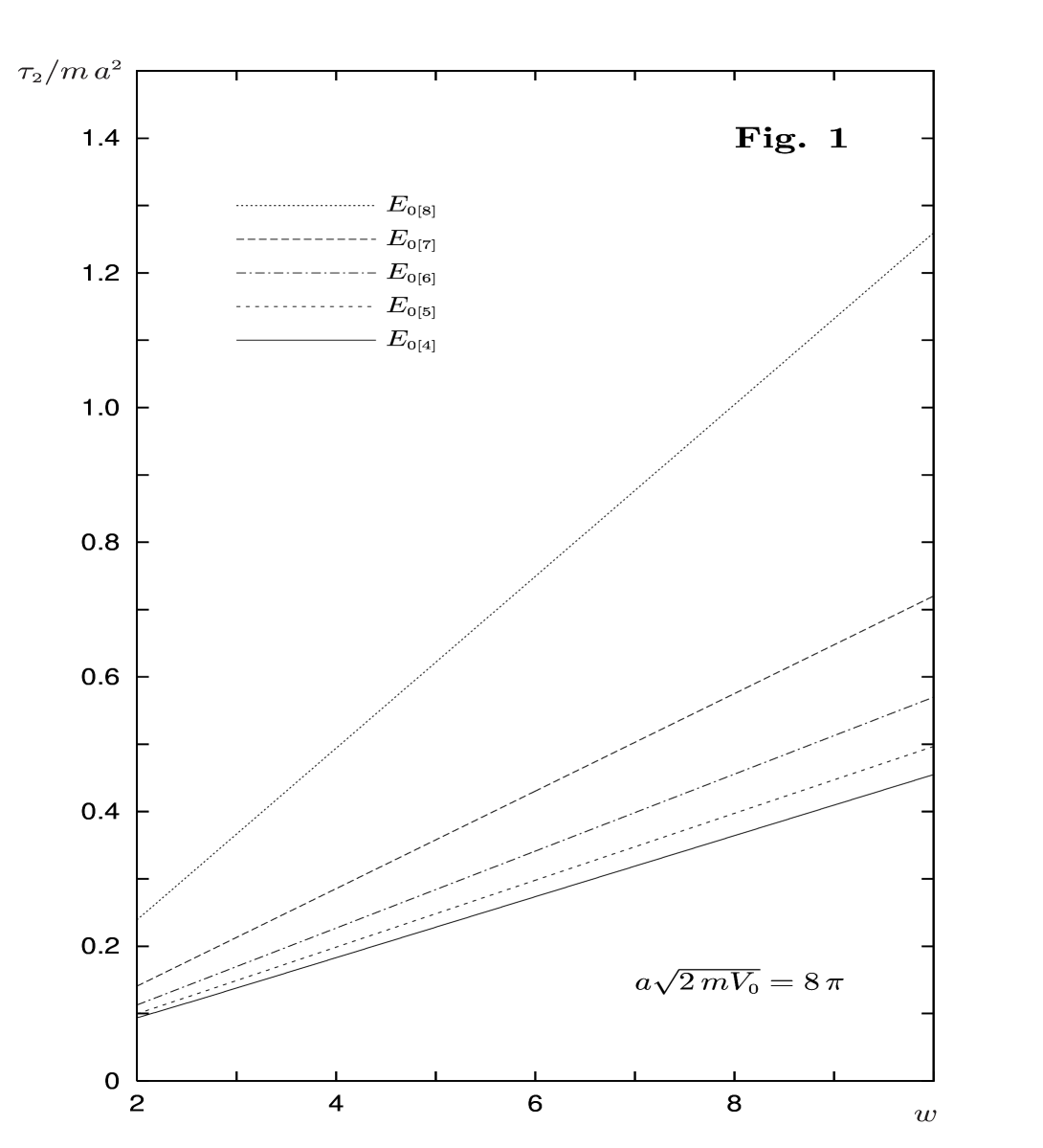
Figure 1: Dependence of $\tau_{\mbox{\tiny$2$}}$ on $w$ for several of the quasi-stationary energies $E_{\mbox{\tiny$0$}}$ of a fixed $V_{\mbox{\tiny$0$}}$

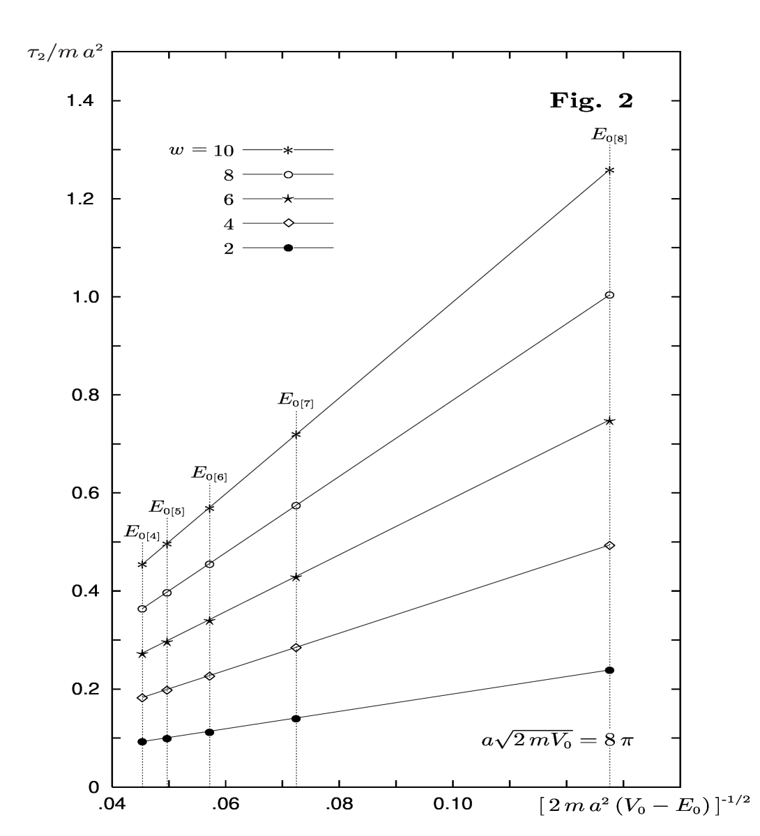
Figure 2: $\tau_{\mbox{\tiny$2$}}$ vs 1/$\sqrt{V_{\mbox{\tiny$0$}}-E_{\mbox{\tiny$0$}}}$ for various quasi-energies $E_{\mbox{\tiny$0$}}$ and $w$ values. The lines drawn demonstrate excellent linear fits, for a fixed $w$.

In Fig. 1 we display the dependence of $\tau_{\mbox{\tiny$2$}}$ upon $w$ for various $E_{\mbox{\tiny$0$}}$ and an arbitrary chosen value of $V_{\mbox{\tiny$0$}}$. In Fig. 2 we show the dependence of $\tau_{\mbox{\tiny$2$}}$ upon $\sqrt{2\,m(V_{\mbox{\tiny$0$}}-E_{\mbox{\tiny$0$}})}$ for different values of $w$. From the above curves we see that, to a very good approximation, $\tau_{\mbox{\tiny$2$}}$ grows linearly with $w$ and hence with the barrier width $b-a$. It is also proportional approximately to $[\,2\,m(V_{\mbox{\tiny$0$}}-E{\mbox{\tiny$0$}})\,]^{\mbox{\tiny$-1/2$}}$. This for the parameter ranges considered. We defer an interpretation of these results to our conclusions.

For $t\rightarrow 0$, the exponential survival law must necessarily lie below the physical curve $P(t)$ if this lacks a linear term since both are normalized to $P(0)=1$. The fact that the lifetime measures the mean time for decay means that an exponential curve with said lifetime as input must eventually rise above $P(t)$ to compensate for the small time ”short-fall”, i.e. there is a cross-over point. As an aside, we note that the power law in $t$ predicted for $P(t)$ at long times means that any exponentially falling curve must lie below $P(t)$ asymptotically adding another cross-over point. The first cross-over allows for the so-called inverse Zeno effect (IZE)[12]. This says that if a first time measurement is made after this cross-over point (but logically before any second cross-over point) the system will have been found to decay at a rate greater than ”expected”.

First, let us analyze critically this definition. Unlike for the QZE this measurement or these measurements (if repeated at the appropriate time intervals) after the inverse Zeno cross-over only contradicts our expectations based upon the use of an exponential curve with the experimental lifetime. But the choice of exponential is somewhat arbitrary. We can give at least two alternative proposals for the reference exponential curve. The first, which is the most natural phenomenologically, is to refer to an exponential best fit to $P(t)$. This fit almost certainly will not have the exact same lifetime as $P(t)$. The second possibility is that one may compare $P(t)$ with a theoretical single exponential (possibly from a model calculation as in our case). These possibilities distinguish themselves from the original because they do not necessarily have a cross-over point and hence need not imply the conditions for an IZE.

We have a natural choice of exponential in our model, the Breit-Wigner exponential. We have thus looked for cross-over points by confronting $P^{\mbox{\tiny$[4]$}}(t)$ with $P^{\mbox{\tiny$[2]$}}(t)$. In all cases examined they have been found. Thus, even with our choice of exponential the IZE is possible. We can see this more clearly by observing that, in our tables, $y_{\mbox{\tiny$1$}}/y_{\mbox{\tiny$2$}}\ll 1$ and $x_{\mbox{\tiny$1$}}\approx x_{\mbox{\tiny$2$}}$, thus we can approximate Eq. (27) as follows

$$P^{\mbox{\tiny$[4]$}}(t)\approx\exp(-4\,x_{\mbox{\tiny$1$}}y_{\mbox{\tiny$1$}}\tilde{t}\,)\,\left\{\,1+2\,\frac{y_{\mbox{\tiny$1$}}}{y_{\mbox{\tiny$2$}}}\,\left[\,\exp(-2\,x_{\mbox{\tiny$2$}}y_{\mbox{\tiny$2$}}\tilde{t}\,)\,\cos(\alpha+\beta\,\tilde{t}\,)-\cos\alpha\right]\,\right\}\,\,.$$ (33)

Consequently,

$$\frac{P^{\mbox{\tiny$[4]$}}(t)}{P^{\mbox{\tiny$[2]$}}(t)}\approx 1+2\,\frac{y_{\mbox{\tiny$1$}}}{y_{\mbox{\tiny$2$}}}\,\varphi(t)\,\,,$$ (34)

where

$$\varphi(t)=\exp\left(-2\,\frac{x_{\mbox{\tiny$2$}}y_{\mbox{\tiny$2$}}}{ma^{\mbox{\tiny$2$}}}\,t\right)\,\cos\left(\alpha+\frac{\beta}{ma^{\mbox{\tiny$2$}}}\,t\right)-\cos\alpha\,\,.$$

Intersection points occur when $\varphi(t)=0$, i.e. when

$$\exp\left(2\,\frac{x_{\mbox{\tiny$2$}}y_{\mbox{\tiny$2$}}}{ma^{\mbox{\tiny$2$}}}\,t\right)=\cos\left(\alpha+\frac{\beta}{ma^{\mbox{\tiny$2$}}}\,t\right)/\cos\alpha\,\,.$$ (35)

The trivial solution is, of course, $t=0$. The condition for the IZE can be determined from the relative values of the time derivative of the functions on the left and right hand sides of the above equation at $t=0$. The necessary and sufficient condition for a non-trivial intersection is

$$2\,x_{\mbox{\tiny$2$}}y_{\mbox{\tiny$2$}}<-\,\beta\,\tan\alpha\,\,.$$ (36)

This is because, with this condition satisfied, the exponential starts off with a flatter growth than the oscillating and bounded right hand side of Eq.(35), and hence they must necessarily cross.

If $x_{\mbox{\tiny$1$}}=x_{\mbox{\tiny$2$}}$ ($\Rightarrow\sin\alpha=0$), we find only the trivial solution $t=0$. On the other hand, from an examination of Table 1, we see that

$$-\,\beta\,\tan\alpha=2\,\frac{\left(x_{\mbox{\tiny$1$}}^{\mbox{\tiny$2$}}-x_{\mbox{\tiny$2$}}^{\mbox{\tiny$2$}}+y_{\mbox{\tiny$2$}}^{\mbox{\tiny$2$}}-y_{\mbox{\tiny$1$}}^{\mbox{\tiny$2$}}\right)\left(x_{\mbox{\tiny$1$}}-x_{\mbox{\tiny$2$}}\right)\left(y_{\mbox{\tiny$1$}}+y_{\mbox{\tiny$2$}}\right)}{\left(x_{\mbox{\tiny$1$}}-x_{\mbox{\tiny$2$}}\right)^{\mbox{\tiny$2$}}-\left(y_{\mbox{\tiny$1$}}+y_{\mbox{\tiny$2$}}\right)^{\mbox{\tiny$2$}}}\approx 2\,x_{\mbox{\tiny$2$}}y_{\mbox{\tiny$2$}}\,\left[1-\left(\frac{y_{\mbox{\tiny$2$}}}{x_{\mbox{\tiny$1$}}-x_{\mbox{\tiny$2$}}}\right)^{\mbox{\tiny$2$}}\,\right]^{-\mbox{\tiny$1$}}\gg 2\,x_{\mbox{\tiny$2$}}y_{\mbox{\tiny$2$}}\,\,.$$

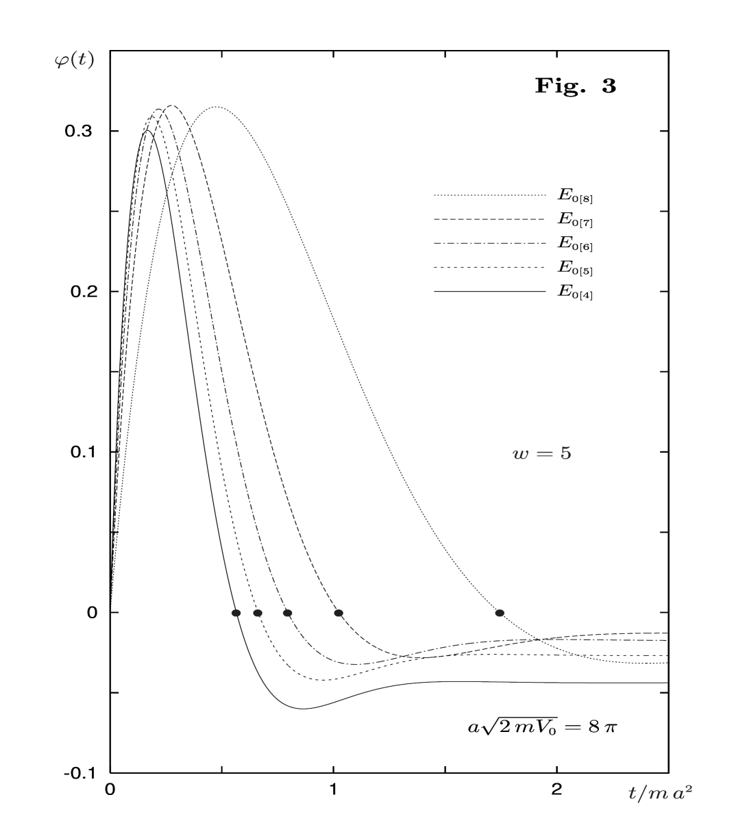
Figure 3: The function $\varphi(t)$ vs $t$ for the indicated values of $V_{\mbox{\tiny$0$}}$ and $\omega$. The five curves are for different values of $E_{\mbox{\tiny$0$}}$ . For each of the curves the cross-over points are indicated by the large dots.

Hence a cross-over occurs for all our tabulated cases. In Fig. 3 we show examples of this by plotting $\varphi(t)$ against $t$ for several quasi-stationary states $E_{\mbox{\tiny$0$}}$ of a fixed barrier height $V_{\mbox{\tiny$0$}}$ and an arbitrary chosen value of $w$. The large dots identify the cross-over times.

VI. CONCLUSIONS

We have discussed in this paper the survival law and its relevance to the QZE and the IZE within the context of a simple potential model. We have shown that the general arguments that allow for the QZE based upon the hermiticity of the Hamiltonian are indeed valid in this model unless one makes very specific assumptions and/or approximations. In particular, the exponential law, which does not allow for the QZE, is obtained only if two approximations are made:

1 - The denominator $f(\sigma)$ in the spectral integral for the amplitude of non-decay is so highly peaked about the initial quasi-state that only the lowest - second order - terms in $\Delta\sigma$ need be considered;

2 - The integral in energy $E$ or equivalently $\sigma$ is extended below the threshold to $-\infty$.
Point 2 is made in order to apply the theorem of residues essential for deriving a single potential survival law. It is also the cause of loss of analyticity in $t$, although this is normally ignored by arguing that only positive values of $t$ are physically significant.

Our analysis has gone on to show that while point 1 (the Breit-Wigner spectrum) is not the sole cause for the theoretical lose of the QZE, it is the primary one. Indeed, if one includes higher order corrections, such as the fourth order terms in $\Delta\sigma$, then the resultant $P^{\mbox{\tiny$[4]$}}(t)$ displays the absence of linear term in $t$, however small the extra contributions might be.

This result was somewhat of a surprise. One could have reasonably supposed that only in the limit of an exact calculation, i.e. when all orders of $\Delta\sigma$ are included, is the linear term absent. Indeed the authors only expected that to fourth order the coefficient of the linear term would be reduced when compared to that of the exponential curve. Instead we have been able to show that it is rigorously null already in $P^{\mbox{\tiny$[4]$}}(t)$. Note that to prove this we have applied points 2 and 3. Point 2 is also significant for another reason. It is known to be the cause for the lose of the long-time power law behavior, and this is independent of any other approximation made. Our conclusions upon the question of the theoretical prerequisite for the QZE is that it is indeed a feature of $P(t)$ and that one must make very specific assumptions or approximations to avoid this effect. Only with the explicit exclusion of short and long times, can a single exponential curve be a good approximation to $P(t)$.

We have also considered in the previous Section the question of the existence or otherwise of the IZE. There is in our opinion a measure of ambiguity in the condition for the existence of this effect because of a non unique choice of the exponential used as reference. Since any exponential is at best an approximation to the physical curve, its definition is subject to discussion. An exponential with the same lifetime as the real curve is the conventional choice. However, there are other choices for which the possible existence of an IZE is far from obvious. We have shown that one possibility, the comparison of $P^{\mbox{\tiny$[4]$}}(t)$ with $P^{\mbox{\tiny$[2]$}}(t)$, does indeed allow for an IZE. Nevertheless, we do not consider the IZE and the QZE comparable phenomena. The former (IZE) refers to our ”expectations”, and as we have argued our expectations are subject to some ambiguity. The latter (QZE) predicts a physical suppression of decay through continuous observation and it is completely independent of the existence or otherwise of an approximate exponential curve.

Of particular interest in our results is the dependence of the second exponential time parameter $\tau_{\mbox{\tiny$2$}}$. The first time parameter $\tau_{\mbox{\tiny$1$}}$ is essentially the lifetime of the system and has a characteristic exponential rise with barrier width $b-a$, whereas this second time parameter can be phenomenological represented by

$$\tau_{\mbox{\tiny$2$}}\approx\frac{ma^{\mbox{\tiny$2$}}\,w}{\sqrt{2\,ma^{\mbox{\tiny$2$}}(V_{\mbox{\tiny$0$}}-E_{\mbox{\tiny$0$}})}}=\frac{m\,(b-a)}{\sqrt{2\,m(V_{\mbox{\tiny$0$}}-E_{\mbox{\tiny$0$}})}}\,\,.$$ (37)

This form is very suggestive. Consider an energy eigenstate above the barrier, $E>V_{\mbox{\tiny$0$}}$. In the barrier region $(a<r<b)$ the particle will have velocity $v=\sqrt{2\,m(E-V_{\mbox{\tiny$0$}})}/m$. Consequently the time taken in crossing the barrier will be:

$$\Delta t=\frac{m(b-a)}{\sqrt{2\,m(E-V_{\mbox{\tiny$0$}})}}.$$ (38)

This ”mirrors” the expression for $\tau_{\mbox{\tiny$2$}}$ (except for the feature that $E_{\mbox{\tiny$0$}}$ has a discrete spectrum). Both tend to infinity if the particle energy and potential energy are set equal. A type of consistency condition. Furthermore, both grow linearly with barrier width. This tempts us to speculate (and at this stage it is no more than an hypothesis) that $\tau_{\mbox{\tiny$2$}}$ is a measure of the time that the particle takes to tunnel free. Equivalently, we may say that $\tau_{\mbox{\tiny$2$}}$ is the time during which the particle is neither bound nor free[7]. However, since this infringes upon the question of transit times and super-luminal velocities [13], which is a very topical, but also complex subject, we desist from any further considerations at this point. The tau are not the only time parameters in $P^{\mbox{\tiny$[4]$}}(t)$, we also have 1/$\beta$ in the oscillatory term. Mathematically it is the natural consequence of interference between the two exponentials of the non-decay amplitude. It is therefore a wave-like property of the particle.

ACKNOWLWDGEMENTS. The authors wish to thank Giampaolo Cò and Piergiulio Tempesta for several comments during the preparation of this manuscript and Saverio Pascazio for helpful suggestions upon the revised version. One of the authors (SDL) also gratefully acknowledges the FAEP (University of Campinas), INFN (Theoretical Group) and MIUR (Department of Physics) for financial support during his stay at the University of Lecce where this paper was prepared.

Table 1: Numerical values of $x_{\mbox{\tiny$1$},\mbox{\tiny$2$}}$ , $y_{\mbox{\tiny$1$},\mbox{\tiny$2$}}$ and $\tau_{\mbox{\tiny$1$},\mbox{\tiny$2$}}$ for chosen values of $V_{\mbox{\tiny$0$}}$. Each block lists the parameters for all the quasi-stationary eigenvalues $E_{\mbox{\tiny$0$}}$.

References

- [1] C. Cohen-Tannoudji, B. Diu and F. Lalöe, Quantum Mechanics (John Wiley & Sons, Paris, 1977), pag.1343.
- [2] R. G. Winter, Phys. Rev. 123, 1503 (1961). S. R. Wilkinson, C. F. Bharucha, M. C. Fischer, K. W. Madison, P. R. Morrow, Q. Niu, B. Sundaram, and M. G. Raizen, Nature 387, 575 (1997); Q. Niu and M. G. Raizen, Phys. Rev. Lett. 80, 3491 (1998); M. C. Fisher, B. Guitérrez, and M. G. Raizen 87, 040402 (2001);
- [3] A. Beskow and J. Nilsson, Arkiv. Fys. 34, 561 (1967); L. Fonda and G. C. Ghirardi, Nuovo Cimento A 7, 180 (1972); C. N. Friedman, Indiana Univ. Math. J. 21, 275 (1972); K. Gustafson and B. Misra, Lett. Math. Phys. 1, 275 (1976); A.Peres, Am. J. Phys. 48, 931 (1980); K. Kraus, Found. Phys. 11, 547 (1981); A. Sudbery, Ann. Phys. 157, 512 (1984); R. J. Cook, Phys. Scr. T. 21, 49 (1988); L. Maiani and M. Testa, Ann. Phys. 263, 353 (1998).
- [4] B. Misra and E. C. G. Sudarshan, J. Math. Phys. 18, 756 (1977).
-
[5]
L. Fonda, G. C. Ghirardi, A. Rimini and T. Weber,
Nuovo Cimento A
15, 689 (1973);
ibidem 18, 805 (1973); C. B. Chiu, E. C. G. Sudarshan and B. Misra, Phys. Rev. D 16, 520 (1977). - [6] W. M. Itano, D. J. Heinzen, J. J. Bollinger and D. J. Wineland, Phys. Rev. A 41, 2295 (1990); P. Kwiat, H. Weinfurter, T. Herzog, A. Zeilinger, and M. Kasevich, Phys. Rev. Lett. 74, 4763 (1995); B. Nagels, L. J. F. Hermans, and P. L. Chapovsky, Phys. Rev. Lett. 79, 3097 (1997); P. E. Toschek and C. Wunderlich, Eur. Phys. J. D 14, 387 (2001).
- [7] S. De Leo and P. Rotelli, JETP Lett. 76, 56 (2002).
- [8] L. A. Khalfin, JETP Lett. 6, 65 (1968).
- [9] H. Nakazato, M. Namiki and S. Pascazio, Int. J. Mod. Phys. B 10, 247 (1996).
- [10] I.I. Gol’dman and U.D. Krivchenkov, Problems in quantum mechanics (Dover, NY, 1961).
- [11] P. Facchi and S. Pascazio, ”Unstable systems and quantum and Zeno phenomena in quantum field theory” (quant-ph/0202127) in Quantum Probability and Withe Noise Analysis XVII, 222 (2003).
- [12] A. M. Lane, Phys. Lett. A 99, 359 (1983); W. C. Schieve, L. P. Horwitz, and J. Levitan, Phys. Lett. A 136, 264 (1989); A. G. Kofman and G. Kurizki, Nature 405, 546 (2000); B. Elattari and S. A. Gurvitz, Phys. Rev. A 62, 032102 (2000); P. Facchi, H. Nakazato and S. Pascazio, Phys. Rev. Lett. 86, 2699 (2001).
- [13] T. E. Hartman, J. Appl. Phys. 33 3427 (1962); V. S. Olkhovsky V. S. and E. Recami, Phys. Rep. 214, 340 (1992); V. S. Olkhovsky, E. Recami and G. Salesi, Europhys. Lett. 56, 879 (2002); Y. Aharonov, N. Erez and B. Reznik, Phys. Rev. A 65, 052124 (2002); S. Esposito, Phys.Rev. E 67, 016609 (2003).