Stability of atomic clocks based on entangled atoms

Abstract

We analyze the effect of realistic noise sources for an atomic clock consisting of a local oscillator that is actively locked to a spin-squeezed (entangled) ensemble of $N$ atoms. We show that the use of entangled states can lead to an improvement of the long-term stability of the clock when the measurement is limited by decoherence associated with instability of the local oscillator combined with fluctuations in the atomic ensemble’s Bloch vector. Atomic states with a moderate degree of entanglement yield the maximal clock stability, resulting in an improvement that scales as $N^{1/6}$ compared to the atomic shot noise level.

Quantum entanglement is the basis for many of the proposed applications of quantum information science bouwmeester . The experimental implementation of these ideas is challenging since entangled states are easily destroyed by decoherence. To evaluate the potential usefulness of entanglement it is therefore essential to include a realistic description of noise in experiments of interest. Although decoherence is commonly analyzed in the context of simple models gardiner , practical sources of noise often possess a non-trivial frequency spectrum, and enter through a variety of different physical processes. In this Letter, we analyze the effect of realistic decoherence processes and noise sources in an atomic clock that is actively locked to a spin-squeezed (entangled) ensemble of atoms.

The performance of an atomic clock can be characterized by its frequency accuracy and stability. Accuracy refers to the frequency offset from the ideal value, whereas stability describes the fluctuations around, and drift away from the average frequency. To improve the long-term clock stability, it has been suggested to use entangled atomic ensembles wineland93 ; wineland94 ; wineland96 , and in this letter we analyze such proposals in the presence of realistic decoherence and noise. In practice, an atomic clock operates by locking the frequency of a local oscillator (L.O.) to the transition frequency between two levels in an atom. This locking is achieved by a spectroscopic measurement determining the L.O. frequency offset $\delta\omega$ from the atomic resonance, followed by a feedback mechanism which steers the L.O. frequency so as to null the mean frequency offset. The problem of frequency control thus combines elements of quantum parameter estimation theory and control of stochastic systems via feedback mabuchi ; wiseman .

The spectroscopic measurement of the atomic transition frequency is typically achieved through Ramsey spectroscopy ramsey , in which the atoms are illuminated by two short, near-resonant pulses from the local oscillator, separated by a long period of free evolution, referred to as the Ramsey time $T$. During the free evolution the atomic state and the L.O. acquire a relative phase difference $\delta\phi=\delta\omega T$, which is subsequently determined by a projection measurement. If a long time $T$ is used, then Ramsey spectroscopy provides a very sensitive measurement of the L.O. frequency offset $\delta\omega$ footnote1 . Here, we investigate the situation relevant to trapped particles, such as atoms in an optical lattice katori or trapped ions wineland00 . In this situation, the optimal value of $T$ is determined by atomic decoherence (caused by imperfections in the experimental setup) which therefore determines the ultimate performance of the clock.

We consider an ensemble of $N$ two-level particles with lower (upper) state $|\downarrow\rangle$ ($|\uparrow\rangle$). Adopting the nomenclature of spin-1/2 particles, we introduce the total angular momentum (i.e., Bloch vector) $\vec{J}=\sum_{j=1}^{N}\vec{S}_{j}$, where e.g. $S_{z}^{j}=\left(|\uparrow\rangle_{j}\langle\uparrow|-|\downarrow\rangle_{j}\langle\downarrow|\right)/2$. Initially the state of the atoms has mean $\langle\vec{J}\rangle$ along the $z$ direction and $\langle J_{x}\rangle=\langle J_{y}\rangle=0$. Unavoidable fluctuations in the $x$ and $y$ components $\langle J_{x}^{2}\rangle=\langle J_{y}^{2}\rangle\neq 0$, result in the so-called atomic projection noise. These fluctuations give rise to an uncertainty in the Ramsey phase $\delta\phi_{R}\simeq\Delta J_{y}/|\langle\hat{J}_{z}\rangle|$ as indicated geometrically in Fig. 1 santarelli99 ; wineland93 . For uncorrelated spins aligned along the $z$ axis, the uncertainty from independent spins are added in quadrature, resulting in the projection noise $\Delta J_{y}=\sqrt{N}/2$. To reduce the measurement error it has been proposed wineland94 ; kitagawa93 ; sorensen01 and demonstrated meyer01 to use entangled atomic states (so called spin squeezed states), which have reduced noise in one of the transverse spin components (e.g., $J_{y}$) and non-zero noise $\Delta J_{z}$ in the mean spin direction. Ideally this gives an improvement by a factor $\xi=\sqrt{N}\Delta J_{y}/\langle J_{z}\rangle$, which can be as low as $\xi=1/\sqrt{N}$ for maximally entangled states wineland96 .

Using a simple noise model it was shown in Ref. huelga97 that entanglement provides little gain in spectroscopic sensitivity in the presence of atomic decoherence. In essence, random fluctuations in the phase of the atomic coherence cause a rapid smearing of the error contour in Fig. 1a. For example, dephasing of individual particles results in an additional contribution $(N/4)\langle\delta\phi^{2}\rangle$ to the noise, where $\langle\delta\phi^{2}\rangle$ denotes the variance of the phase fluctuations (increasing with $T$ as $\langle\delta\phi^{2}\rangle=\gamma T$ for white noise, where $\gamma$ is the dephasing rate). In practice, the stability of atomic clocks is often limited primarily by fluctuations of the L.O. As we show below, the L.O. fluctuations result in the added noise $\Delta J_{z}^{2}\langle\delta\phi^{2}\rangle$, where $\Delta J_{z}^{2}$ is the initial variance in $J_{z}$. This added noise is due to the error in the feedback loop, caused by the longitudinal noise $\Delta J_{z}$. For weakly entangled states, the added noise is considerably smaller than in the case of atomic dephasing and the use of entangled states can lead to a significant improvement in clock stability.

In what follows we outline a model that incorporates the effects of atomic noise and spin squeezing as well as that of the feedback loop. Before proceeding, we note that qualitative considerations along these lines were noted in Ref. winelandbible . At the operating point, the error signal in Ramsey spectroscopy wineland94 measured at time $t_{k}$ is determined by the operator

$$\hat{E}(t_{k})\simeq\sum_{j=1}^{N}\hat{S}_{z}^{j}\sin[\delta\phi_{j}(t_{k})]+\hat{S}_{y}^{j}\cos[\delta\phi_{j}(t_{k})],$$ (1)

where $\delta\phi_{j}(t_{k})$ is the phase acquired by the $j$th atom during the interrogation time $T$ and all operators refer to the initial atomic state. We separate the phase into two parts $\delta\phi_{j}=\delta\phi_{O}+\delta\phi_{E}^{j}$, where $\delta\phi_{O}(t_{k})=\int_{0}^{T}\delta\omega(t_{k}-t)dt$ is the phase due to the frequency fluctuations $\delta\omega(t)$ of the L.O., and $\delta\phi_{E}^{j}$ is a phase induced by the interaction of the $j$th atom with the environment. In order to lock the L.O. to the atomic frequency, the interrogation time should be short enough that $\langle\delta\phi(t_{k})^{2}\rangle\lesssim 1$. Expanding in terms of $\delta\phi(t_{k})$, we find the measured error signal

$$\mathcal{E}(t_{k}) \simeq \langle\hat{J}_{z}\rangle\left(\delta\phi_{O}(t_{k})-\frac{\delta\phi_{O}(t_{k})^{3}}{3!}\right)+\sum_{j=1}^{N}\mathcal{S}_{z}^{j}\delta\phi_{E}^{j}(t_{k})$$ (2)

$$+ [\mathcal{J}_{y}(t_{k})+\delta\mathcal{J}_{z}(t_{k})\delta\phi_{O}(t_{k})]+\cdots.$$

Here $\delta\mathcal{J}_{z}(t_{k})=\mathcal{J}_{z}(t_{k})-\langle\hat{J}_{z}\rangle$, where $\mathcal{J}_{z}(t_{k})$ and $\mathcal{J}_{y}(t_{k})$ are random numbers with a distribution corresponding to the initial atomic state (we consider here states for which $\langle\hat{J}_{y}\hat{J}_{z}\rangle=0$, so that we may treat $\mathcal{J}_{z}(t_{k})$ and $\mathcal{J}_{y}(t_{k})$ as independent random variables). The term multiplying $\langle\hat{J}_{z}\rangle$ in (2) is used to estimate the frequency offset, while the remaining terms represent measurement noise.

The feedback is started at $t=0$ and, at the end of each Ramsey cycle, at $t_{k}=kT$ ($k=1,2,...$), the detection signal is used to steer the frequency of the oscillator to correct for the fluctuations accumulated during the last cycle $\delta\omega(t_{k}^{+})=\delta\omega(t_{k}^{-})+\Delta\omega(t_{k})$, where $t_{k}^{-}$ and $t_{k}^{+}$ refer to before and after the correction, and $\Delta\omega(t_{k})$ is the frequency correction. Assuming that negligible time is spent performing the $\pi/2$ pulses and in preparing and detecting the state of the atoms, the mean frequency offset after running for a period $\tau=nT$ is then

$$\delta{\bar{\omega}}(\tau) = \frac{1}{\tau}\int_{0}^{\tau}\delta\omega(t)dt$$ (3)

$$= \frac{T}{\tau}\sum_{k=1}^{n}\left[\frac{\delta\phi_{O}(t_{k})}{T}+\Delta\omega(t_{k})\right].$$

We begin by analyzing the simplest case of linear feedback (in $\mathcal{E}(t_{k})$) and later extend to the more optimal nonlinear feedback case. With $\Delta\omega(t_{k})=\frac{-\mathcal{E}(t_{k})}{\langle\hat{J}_{z}\rangle T}$, using (2) and substituting in (3), we find, ignoring for now the $\delta\phi_{O}(t_{k})^{3}$ term,

$$\delta{\bar{\omega}}(\tau) = \frac{-1}{\tau\langle\hat{J}_{z}\rangle}\sum_{k=1}^{n}[\mathcal{J}_{y}(t_{k})+\delta\mathcal{J}_{z}(t_{k})\delta\phi_{O}(t_{k})$$ (4)

$$+ \sum_{j=1}^{N}\mathcal{S}_{z}^{j}\delta\phi^{j}_{E}(t_{k})]$$

Note that the acquired offsets $\delta\phi_{O}(t_{k})/T$ ($k=1,...,n$) due to L.O. frequency fluctuations are corrected by the feedback loop and do not appear in (4), while measurement noise is added at the detection times $t_{k}$. The first two terms in (4) are uncorrelated for different $t_{k}$ since the atomic noise for different detection events is uncorrelated. If the dephasing noise is uncorrelated for different $t_{k}$, then the fractional frequency fluctuation (Allan deviation) barnes71 $\sigma_{y}(\tau)=\langle(\delta{\bar{\omega}}(\tau)/\omega)^{2}\rangle^{1/2}$, is

$$\sigma_{y}(\tau)=\frac{\left[\Delta J_{y}^{2}+\Delta J_{z}^{2}\langle\delta\phi_{O}^{2}\rangle+(\lambda\langle J_{z}^{2}\rangle)\langle\delta\phi_{E}^{2}\rangle\right]^{1/2}}{\omega\sqrt{\tau T}\langle\hat{J}_{z}\rangle}.$$ (5)

Here $\lambda$ accounts for the possibility of collective decoherence, so that for atoms dephasing collectively (independently) $\lambda\rightarrow 1$ ($\lambda\rightarrow(N/4)/\langle\hat{J}_{z}^{2}\rangle$). The L.O. noise affects the atoms in a similar fashion than collective dephasing. Note, however, the significant difference between collective environmental dephasing, which enters expression (5) as $\langle\hat{J}_{z}^{2}\rangle\langle\delta\phi_{E}^{2}\rangle$, and L.O. noise, for which $\Delta J_{z}^{2}\langle\delta\phi_{O}^{2}\rangle$ is the relevant expression. The feedback loop results in a large cancellation of the effect of the L.O. noise on the stability; the uncanceled part of the noise is now proportional to $\Delta J_{z}^{2}\ll\langle\hat{J}_{z}^{2}\rangle$.

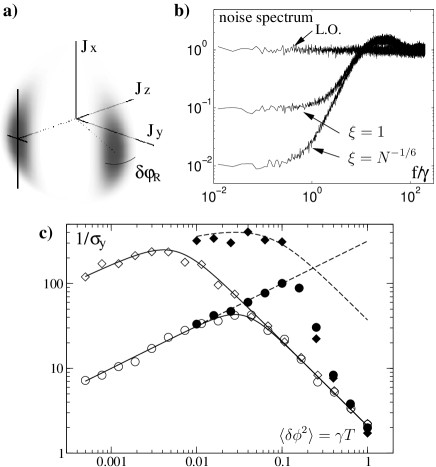
Figure 1: a) Representation of the probability distribution on the Bloch sphere for a spin squeezed state $|\psi(\kappa)\rangle$, with $\kappa=N^{1/4}$ corresponding to the squeezing parameter $\xi=N^{-1/4}$ ($N=10$, both the initial state and the state just before detection are shown for clarity). Thick lines indicate initial uncertainties in $\vec{J}$. b) Noise spectra due to L.O. frequency fluctuations when free running, when stabilized to unsqueezed atoms ($\xi=1$), and when stabilized to spin squeezed atoms ($\xi=N^{-1/6}$), $N=10^{3}$ and $\gamma T=10^{-2}$. c) Inverse fractional frequency stability $1/\sigma_{y}$ (arbitrary units) vs. Ramsey time for white L.O. noise, $N=10^{5}$, with linear feedback to uncorrelated atoms ($\circ$); linear feedback to correlated atoms ($\diamond$, $\xi=N^{-1/4}$); nonlinear feedback to uncorrelated atoms ($\bullet$); and nonlinear feedback to correlated atoms (filled $\diamond$, $\xi=N^{-1/4}$). Points: numerical simulations, lines: analytical results.

When decoherence is negligible, $\langle\delta\phi_{O}^{2}\rangle=\langle\delta\phi_{E}^{2}\rangle=0$, the long term frequency stability is given by $\sigma_{y}(\tau)={\Delta J_{y}}/{\omega\sqrt{\tau T}\langle\hat{J}_{z}\rangle}$ as shown in Refs. wineland93 ; wineland94 . For an uncorrelated atomic state, the stability improves with increasing number of atoms as $N^{-1/2}$ santarelli99 . The maximum possible improvement using spin-squeezed states is a factor of $N^{-1/2}$, yielding a stability $\sigma_{y}(\tau)\propto N^{-1}$ wineland96 .

The best long term stability is obtained with the longest possible interrogation time $T$. When the interrogation time is limited by environmental decoherence, the latter cannot be ignored. This corresponds to the situation considered in Refs. huelga97 ; kitagawa01 , in which case no substantial improvement is possible. In the practically relevant case where the main source of noise is from the L.O. wineland98 ; wineland00 ; wineland01_2 the situation is quite different. In this case it is undesirable to use a very highly squeezed state with $\Delta J_{y}\sim 1$ because it has a very large uncertainty in the $z$-component of the spin $\Delta J_{z}\sim N$, which according to Eq. (5) has a large contribution to the noise. A moderately squeezed state can, however, lead to a considerable improvement in the stability. This observation is the main result of the present Letter.

To find the optimal stability, we first optimize (5) with respect to the interrogation time. Considering uncorrelated atoms first, we have $\Delta J_{y}=\sqrt{N}/2$ and $\Delta J_{z}=0$; Eq. (5) then predicts that $\sigma_{y}(\tau)$ decreases indefinitely as $1/\sqrt{T}$. To derive Eq. (5), however, we have linearized the expression in Eq. (1), and this linearization breaks down when the (neglected) cubic term in (2) is comparable to the noise term that we retained, i.e., when $\delta\phi(t_{k})^{3}\sim\Delta J_{y}/\langle\hat{J}_{z}\rangle$. In a more careful analysis longpaper based on Eq. (2), including perturbatively the nonlinear terms in a stochastic differential equation, we find the optimal time $\gamma T=(2\Delta J_{y}^{2}/\langle\hat{J}_{z}\rangle^{2})^{1/3}$. At this point the stability is given by $\sigma_{y}(\tau)=\zeta N^{-1/3}\gamma/{\omega\sqrt{\gamma\tau}}$ where

$$\zeta=\frac{3}{2^{4/3}}N^{1/3}\left[\left(\frac{\Delta J_{y}}{\langle\hat{J}_{z}\rangle}\right)^{4/3}+\frac{2^{4/3}}{3}\left(\frac{\Delta J_{z}}{\langle\hat{J}_{z}\rangle}\right)^{2}\right]^{1/2}.$$ (6)

To evaluate the potential improvement in stability by using squeezed states (i.e., the scaling with increasing number of atoms $N$, in the limit $N\gg 1$), it is convenient to use a family of states parametrized by a small number of parameters. A one-parameter family of states that includes the uncorrelated state as well as spin squeezed states is given by the Gaussian states $|\psi(\kappa)\rangle={\mathcal{N}(\kappa)}\sum_{m}(-1)^{m}e^{-(m/\kappa)^{2}}|m\rangle$, where $|m\rangle$ are eigenstates of the $J_{y}$ operator with eigenvalue $m$ and the total angular momentum quantum number is $J=N/2$, and $\mathcal{N}(\kappa)$ is a normalization factor. The transverse noise for these states is given by $\Delta J_{y}=\kappa/2$. For a large number of atoms $N\gg 1$, the uncorrelated state is well approximated by $|\psi(\kappa=\sqrt{N})\rangle$, while highly-squeezed states are obtained when $\kappa\rightarrow 1$. Within this family of states the optimal value is $\zeta\simeq 1.42N^{-1/6}$ for $\kappa\simeq 2^{1/16}N^{1/4}$ ($\xi\sim N^{-1/4}$) giving a stability scaling as $N^{-1/2}$. This represents an improvement by a factor of $N^{1/6}$ compared to uncorrelated states, for which $\zeta=3/2^{4/3}$ and the stability scales as $N^{-1/3}$. We emphasize that these results are derived assuming a linear feedback loop.

To confirm these predictions, we have made extensive numerical simulations of the frequency control loop, along the lines of Ref. Audoin98 . The noise spectrum of the free-running oscillator is defined by $S(f)\delta(f+f^{\prime})=\langle\delta\omega(f)\delta\omega(f^{\prime})\rangle$, where $\delta\omega(f)$ is the Fourier transform of the stochastic process $\delta\omega(t)$. We generate the corresponding time-series and at the detection times $t_{k}=kT$, the accumulated phase $\delta\phi_{O}(t_{k})$ is calculated and the atomic noise is generated from the probability distributions of $\mathcal{J}_{y}$ and $\mathcal{J}_{z}$. The error signal $\mathcal{E}(t_{k})$ is found and a frequency correction $\Delta\omega(t_{k})$ is generated. The noise spectrum of the slaved oscillator, see Fig. 1b, clearly shows that while for short time scales ($\lesssim T$, high frequencies) the noise is given by that of the free-running oscillator, at longer time scales (lower frequencies) the oscillator is locked to the atoms and the remaining (white) noise is determined by the atomic fluctuations. The low-frequency white noise floor determines the long-term stability of the clock and is the quantity we seek to optimize. In Fig. 1(c) we compare our analytical results with the results of the numerical simulations as a function of Ramsey time $T$, and in Fig. 2(a) we show the scaling with the number of atoms. The analytical and numerical approaches are in excellent agreement.

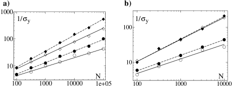
Figure 2: Inverse fractional frequency stability $1/\sigma_{y}$ (arbitrary units) vs. number of atoms $N$, with Ramsey time optimized for a) white noise and b) $1/f$ noise. Points: numerical simulations, lines: analytical results. Uncorrelated atoms ($\circ$) and optimal spin squeezed atoms ($\diamond$), both for linear feedback (full lines, open symbols) and nonlinear feedback (dashed lines, filled symbols).

So far we have assumed linear feedback and white noise; we now relax these assumptions. The stability limit identified above is mainly determined by the breakdown of the assumption of small (i.e., linear) phase fluctuations. In fact, the stability can be improved considerably by using a feedback $\Delta\omega$ which is a nonlinear function of the error signal $\mathcal{E}$. To investigate this we have included a nonlinear feedback $\Delta\omega(t_{k})\propto\arcsin[{\mathcal{E}}(t_{k})/J]$ in our numerical simulations. In Fig. 1(c) it is seen that nonlinear feedback performs better, and that it extends the validity of Eq. (5) all the way to $\gamma T\sim 0.1$. For larger $\gamma T$, the feedback loop fails, resulting in a rapid decrease in stability. If we optimize the Allan deviation in Eq. (5) for nonlinear feedback, under the condition $\gamma T\leq 0.1$, we find that the optimally squeezed states have $\Delta J_{y}\sim N^{1/3}$ ($\xi\sim N^{-1/6}$) resulting in a stability scaling as $N^{-2/3}$. This represents again a relative improvement in scaling of $N^{1/6}$ compared to the uncorrelated state for which the stability scales as $N^{-1/2}$. Detailed derivation of these results will be presented elsewhere longpaper .

The assumption of white noise $\langle\delta\phi^{2}\rangle=\gamma T$, is convenient for theoretical calculations, but in practice very-low-frequency noise is likely to have nontrivial spectrum such as $1/f$ noise. To find the scaling with the number of atoms in this situation, we replace $\langle\delta\phi^{2}\rangle=\gamma T$ with the behaviour expected for $1/f$ noise: $\langle\delta\phi^{2}\rangle\sim(\gamma T)^{2}$. Repeating all the calculations above we again find an improvement by a factor of $N^{1/6}$ by using squeezed states for the nonlinear feedback loop, and a factor of $N^{5/24}$ for linear feedback. In Fig. 2b we compare these scaling arguments to the numerical simulations and the two approaches are seen to be in very good agreement.

To summarize, we have shown that entanglement can provide a significant gain in the frequency stability of an atomic clock when it is limited by the stability of the oscillator used to interrogate the atoms. The optimal stability is achieved by using moderately squeezed states, with a relative improvement that scales approximately as $N^{1/6}$ with the number of atoms. These results are in contrast to previous studies using simplified decoherence models, which found that no practical improvement can be achieved with entangled states. Finally, we note a few interesting questions raised by our work. First, it would be interesting to see if there exists special quantum states of atoms and feedback mechanisms which optimize the performance of the clock. Second, the present results highlight that it is essential to have a realistic model of the noise (and possible stabilization mechanism) present in specific realizations of quantum information protocols. Although the protocol considered in this Letter exploits entanglement to stabilize a classical system (the local oscillator), it would be interesting to study how similar considerations (e.g. $1/f$ noise and collective decoherence) affect protocols such as quantum error correction codes bouwmeester , which use entanglement to stabilize a quantum system and protect it from decoherence.

We are grateful to David Phillips, Ron Walsworth, and David Wineland for useful discussions and comments on the manuscript. This work was supported by the NSF through its CAREER award and the grant to ITAMP, by the Packard and Sloan Foundations, and by the Danish Natural Science Research Council.

References

- (1) D. Bouwmeester, A. Ekert, and A. Zeilinger (eds.), The Physics of Quantum Information, (Springer, New York, 2000).
- (2) C. W. Gardiner and P. Zoller, Quantum Noise, (Springer, New York, 2000).
- (3) W. H. Itano et al., Phys. Rev. A 47, 3554 (1993).
- (4) J. J. Bollinger et al., Phys. Rev. A 54, R4649 (1996).
- (5) D. J. Wineland et al., Phys. Rev. A 50, 67 (1994).
- (6) J. M. Geremia et al., Phys. Rev. Lett. 91, 250801 (2003).
- (7) L. K. Thomsen, S. Mancini, and H. M. Wiseman, Phys. Rev. A 65, 061801 (2002).
- (8) N. F. Ramsey, Molecular Beams, (Oxford University Press, London 1956).
- (9) In practice, may be limited by various mechanisms, e.g., in atomic fountain clocks, is limited by the available distance the atoms may fall under gravity santarelli99 .
- (10) G. Santarelli et al., Phys. Rev. Lett. 82, 4619 (1999).
- (11) M. Takamoto and H. Katori, Phys. Rev. Lett. 91, 223001 (2003).
- (12) R. J. Rafac et al., Phys. Rev. Lett. 85, 2462 (2000).
- (13) M. Kitagawa and M. Ueda, Phys. Rev. A 47, 5138 (1993).
- (14) A. Sørensen, L.-M. Duan, J. I. Cirac, and P. Zoller, Nature 409, 63 (2001).
- (15) V. Meyer et al., Phys. Rev. Lett. 86, 5870 (2001).
- (16) S. F. Huelga et al., Phys. Rev. Lett. 79, 3865 (1997).
- (17) D. J. Wineland el al., J. Res. Natl. Inst. Stan. Technol. 103, 259 (1998).
- (18) A. André, A. S. Sørensen, and M. D. Lukin, (in preparation).
- (19) J. A. Barnes et al., IEEE Trans. Instrum. Meas. 20, 105 (1971).
- (20) D. Ulam-Orgikh and M. Kitagawa, Phys. Rev. A 64, 052106 (2001).
- (21) D. J. Berkeland et al., Phys. Rev. Lett. 80, 2089 (1998).
- (22) S. A. Diddams et al., Science 293, 825 (2001).
- (23) C. Audoin et al., IEEE Trans. Ultrason., Ferroelect., Freq. Contr. 45, 877 (1998); C. A. Greenhall, ibid. 45, 895 (1998).