Local field effects and multimode stimulated light scattering in a two-level medium

Abstract

Scattering of a short (much shorter then the spontaneous lifetime) laser pulse has been considered in a dense resonant medium subject to local field effects. The system was studied in the limit of Hartree-Fock approximation for Bogolubov-Born-Green-Kirkwood-Yvon (BBGKY) hierarchy of equations for reduced density operators. A closed set of equations for atomic and field density operators was derived to describe stimulated scattering of radiation. Numerically as well as theoretically the capability of multicomponent spectrum with maximums multiple to Rabi frequency has been demonstrated. Relative line intensities in the spectrum were found in the limit of low density.

I Introduction.

The properties of scattered light which one can observe under action of a strong laser field have been the area of intensive research in quantum optics. Wigner-Weisskopf 1 were the first to demonstrate that when a two-level system is excited with a weak monochromatic field its fluorescence spectrum was determined by Rayleigh scattering. In this case the criterion for the weak pump field was the ratio of Rabi frequency to either the spontaneous decay rate or detuning from resonance. In strong fields the stimulated (Rayleigh) component is accompanied by spontaneous radiation displaying two additional maximums in the spectrum building the well known Mollow triplet Mollow69 . It must be noted that for stationary pump modes in the strong field limit the coherent component of radiation is reciprocally proportional to the square of Rabi frequency and is, therefore, negligible. These result have found numerous excellent experimental verifications Exp .

The general picture is much more complicated when such a process is studied in dense media. This is mainly due to strong interatomic interactions giving rise to collective behavior of atoms exposed to external laser fields. The pioneer consideration of this issue was presented in work Dike by Dicke who demonstrated that in an optically dense medium of $N$ atoms ($n\lambdabar^{3}\gg 1$, where $n$ is the density of atoms and $\lambdabar=\lambda/2\pi$ $\lambda$ is the wavelength) collective spontaneous decay with its intensity proportional to $N^{2}$ was possible.

One of the most studied range of phenomena in this aspect is linked to the interaction of closely positioned atomic systems through their radiation field and combines a number of well investigated cooperative effects Andreev . This type of phenomena includes local-field effects or the near dipole-dipole interaction, a striking sequence of which is intrinsic optical bistability predicted and studied theoretically Bowden_79 ; Bowden_84-93 ; Bowden_96 ; Bowden_Rev and observed in experiments with impurities embedded into crystalline matrices or doped glasses Crystaline ; Glass . It has been demonstrated that local field effects can notably affect the spontaneous decay rate Bowden_2000 ; Fleischhauer ; Knoll . Also, for these case the strict condition forbidding realization of such bistability mechanism cased by collisional broadening was eliminated Manassah_89 ; Manassah_2001 .

Another area of studies is linked to collective spontaneous decay. In addition to higher decay rate Dike interatomic interaction can substantially modify the spontaneous spectrum in comparison with the single atom case Agarwal77 ; Amin78 . Interaction between the atoms gives rise to additional resonances in absorption and emission spectra which is explained by possibility for simultaneous excitation of different atoms and excitation exchange Senitzky78 ; Carmichael79 ; Agarwal80 ; Drummond80 ; Freedhoff80 ; Ficek81 ; Kilin80 ; Kus81 ; Griffin82 ; Ficek84 .

Additional lines including satellites multiple to Rabi frequency in superradiant spectra was first reported and discussed in Agarwal77 ; Amin78 ; Senitzky78 . However, intensities of such additional sidebands were shown to be utterly small, i.e., $\sim 10^{-6}$ to the central peak. It must be noted that there are some other difficulties found in connection to conditions for the superradiant mode. This fact puts the limitations on the value of the transverse relaxation constant Mandel $\gamma_{2}\ll N\gamma$, where $\gamma$ is the radiative relaxation rate. It all makes it very complicated to observe the sidebands experimentally.

One should note that in the references cited above there was steady state spectra analysis only so the contribution of stimulated scattering (Rayleigh component) in resonance fluorescence has not been considered. On one hand it could have been conditioned by its smallness, but on the other hand in the steady state it is scattered ”elastically”. However, as we demonstrated in Roerich2003 in transient spectra the profile of stimulated scattering is different from delta function and its frequency is not the same as that of the pump field. Besides, its intensity is no small in comparison with that of spontaneous radiation. In dense media, similar to superradiation, intensity is proportional to the square of atomic density and under certain conditions may dominate over spontaneous intensity especially when the superradiant mode is not likely to arise because of collisions.

The aim of this work is to study transient spectra of stimulated scattering in a dense medium excited by a short laser pulse. In the limit of Hartree-Fock approximation applied for BBGKY-hierarchy of equations for the reduced density operators Bonitz we will receive equations of motion for atomic and field density operators which imply local field corrections giving rise to nonlinearities of the system. Expressions describing intensity spectra of scattered light will be also obtained. Using the method of successive approximations we will conduct theoretical analysis of scattered light in case when the medium is excited by a short laser pulse of constant intensity profile. In conclusion we will make a comparison of the analytical solution with the exact solution obtained numerically and study the spectral properties in a wide range of parameters.

This work is structured as follows. In Sec. II we present the approximations to be used and derive the equations of motion for the atomic and field density operators. In Sec. III we apply the method of successive approximations to obtain analytical solutions for the equations and discuss their properties. In Sec. IV the spectrum of scattered light is studied numerically. A comparison with the analytic solution is carried out while the properties of obtained spectra are studied for a wider range of parameters. In the summary we list the basic results. The appendix contains the explicit derivation scheme for the local field operator.

II Basic equations

We will consider interaction of a medium of nondegenerate two-level atoms with a laser field resonant to $1\to 2$ atomic transition. In the dipole and rotative wave approximations the Hamiltonian of the system, describing the interaction of $N$ atoms and laser field, in units $1/\hbar$ has the form:

$$\displaystyle{H=\sum^{N}_{l=1}(H_{a}+V_{a})+\sum_{{\bf k}}H_{f}+\sum^{N}_{l=1}\sum_{{\bf k}}V_{af},}$$ (1)

where

$$\begin{array}[]{c}\displaystyle{H_{a}=\Delta_{21}|2\rangle\langle 2|,\;\;\;\;}\displaystyle{H_{f}=\nu_{\bf k}\hat{a}_{\textbf{k}_{\alpha}}^{+}\hat{a}_{\textbf{k}_{\alpha}},}\\ \displaystyle{V_{af}=i(g_{l}({\bf k}_{\alpha})|2\rangle\langle 1|\hat{a}_{\textbf{k}_{\alpha}}-g_{l}({\bf k}_{\alpha})^{*}|1\rangle\langle 2|\hat{a}_{\textbf{k}_{\alpha}}^{+}),}\\ \displaystyle{V_{a}=i(R(t,{\bf r})|2\rangle\langle 1|-R^{*}(t,{\bf r})|1\rangle\langle 2|).}\end{array}$$ (6)

In (6) $H_{a}$ describes the Hamiltonian of an unperturbed atomic system, $\Delta_{21}=\omega_{21}-\omega_{L}$ is the detuning from resonance, $\omega_{21}$ being the transition frequency and $\omega_{L}$ the carrier frequency of a laser pulse, $|j\rangle,\langle j|,j=1,2$ are the projection operators for respective atomic states.

The next term $H_{f}$ describes the Hamiltonian of quantized radiation field, where $\hat{a}_{\textbf{k}_{\alpha}}^{+},\hat{a}_{\textbf{k}_{\alpha}}$ are formation and annihilation operators respectively; $\nu_{\bf k}=\omega_{\bf k}-\omega_{L}$, $\omega_{\bf k}$ is the frequency of a photon with the wave vector ${\bf k}$ and polarization $\alpha$.

Operator $V_{af}$ describes interaction of atom $l$ with a mode of the quantized field, where $\displaystyle{g_{l}({\bf k}_{\alpha})=\sqrt{\frac{2\pi\omega_{\bf k}}{\hbar W}}}e^{i{\bf k}{\bf r}_{l}}(\vec{\mu}_{21}\epsilon({\bf k}_{\alpha}))$ defines the coupling constant, here $\vec{\mu}_{21}$ is the dipole transition operator, $\epsilon({\bf k}_{\alpha})$ is a unitary polarization vector, and ${\bf k}\cdot\epsilon({\bf k}_{\alpha})=0$, $\alpha=1,2$ $W$ is the quantization volume. Operator $V_{a}$ describes interaction of an atom with the laser field $R(t,{\bf r})=-\displaystyle{\frac{\vec{\mu}_{21}{\bf E}_{L}(t,{\bf r})}{2\hbar}}$, where $E_{L}(t,{\bf r})$ is the laser field strength.

Besides, it is necessary to introduce an operator which describes radiative absorption by the cavity walls related to either operation of a detector device or whatever else irretrievable loss of radiation. Allowing for the losses brings an additional term to the Hamiltonian (6) having the form $\sum_{\bf k}K_{\bf k}[\rho]$ and describing interaction of the quantized field with thermostat at zero temperature Perelomov :

$$K_{\bf k}[\rho]=-i\eta_{\bf k}/2(\hat{a}_{\textbf{k}_{\alpha}}^{+}\hat{a}_{\textbf{k}_{\alpha}}\rho-2\hat{a}_{\textbf{k}_{\alpha}}\rho\hat{a}_{\textbf{k}_{\alpha}}^{+}+\rho\hat{a}_{\textbf{k}_{\alpha}}^{+}\hat{a}_{\textbf{k}_{\alpha}}),$$ (7)

where $\eta_{\bf k}$ determines the mode losses.

In order to obtain equations describing the spectrum of scattered light we will use the BBGKY-hierarchy in the framework of Hartree-Fock approximation applying the well-known cluster expansion for reduced density operators Bonitz . While carrying out the derivation steps we will neglect the spontaneous radiation and collisional relaxation considering the laser pulse duration sufficiently small. However, we take into account the fact that the resonant medium can be dense enough, i.e., $n({\bf r})\lambda_{21}^{3}/8\pi^{3}\gg 1$ to let the local (cooperative) field effects to be strong. Here, $n({\bf r})$ is the density and $\lambda_{21}$ is the transition wavelength. We will further neglect spontaneous scattering as its intensity is low if compared with that of the simulated scattering being proportional to the squared density Roerich2003 .

We assume that initially the atoms are not perturbed which makes it possible to represent the atom-field density operator as the product of atomic and field parts:

$$\rho=\prod_{N}{\rho_{0}^{a}}({\rho_{11}^{a}}=1)\prod_{{\bf k}_{\alpha}}|0_{{\bf k}_{\alpha}}\rangle\langle 0_{{\bf k}_{\alpha}}|.$$ (8)

In the view of approximation taken above the BBGKY-hierarchy takes the form :

$$\begin{array}[]{c}\displaystyle{i\frac{d{\rho^{a}}}{dt}}-[H_{a}+V_{a},{\rho^{a}}]-[V_{af^{{}^{\prime\prime}}},{\rho^{a}}\rho_{f^{{}^{\prime\prime}}}]^{f^{{}^{\prime\prime}}}=0,\\ \displaystyle{i\frac{d\rho_{f}}{dt}}-[H_{f}^{r},\rho_{f}]-K_{\bf k}[\rho_{f}]-[V_{a^{{}^{\prime\prime}}f},\rho_{a^{{}^{\prime\prime}}}\rho_{f}]^{a^{{}^{\prime\prime}}}=0,\\ {\rho^{a}}(0)={\rho_{0}^{a}},\;\;\;\;\rho_{f}(0)=|0_{{\bf k}_{\alpha}}\rangle\langle 0_{{\bf k}_{\alpha}}|,\\ \end{array}$$ (12)

where ${\rho^{a}},\rho_{f}$ are atomic and field single particle density operators respectively; $[.]^{f},[.]^{a}$ denote tracing operation over field and atomic variables with $[.]$ being usual commutator brackets. The BBGKY-hierarchy in this approximation is comprised of a Bloch equation for two-level atoms interacting with laser field complemented with the term $[V_{af},{\rho^{a}}\rho_{f}]^{f}$ which is responsible for the feedback to the atom from the scattered light and the field equation written in Shrodinger representation. Here, the term $[V_{af},{\rho^{a}}\rho_{f}]^{a}$ is the quantum representation of field induced atomic polarization.

In order to find a solution for the system (12) we will use the transformation which already used in papers Roerich2003 . At first, however, it is expedient to change to the wave picture by means of the substitution $\rho_{f}=e^{-iH_{f}^{r}t}\rho_{f}^{(1)}e^{iH_{f}^{r}t}$. As the result, the system (12) now reads

$$\begin{array}[]{c}\displaystyle{i\frac{d{\rho^{a}}}{dt}}-[H_{a}+V_{a},{\rho^{a}}]-[\tilde{V}_{af},{\rho^{a}}\rho_{f}^{(1)}]^{f}=0,\\ \displaystyle{i\frac{d\rho_{f}^{(1)}}{dt}}-K_{\bf k}[\rho_{f}^{(1)}]-[\tilde{V}_{af},{\rho^{a}}\rho_{f}^{(1)}]^{a}=0,\\ \displaystyle{\tilde{V}_{af}=ig_{l}({\bf k}_{\alpha})|2\rangle\langle 1|\hat{a}_{\textbf{k}_{\alpha}}e^{-i\nu_{k}t}+H.c.}.\\ \end{array}$$ (16)

Let us write out explicitly the operator describing the induced atomic polarization:

$$\begin{array}[]{c}\displaystyle{[\tilde{V}_{af},{\rho^{a}}\rho_{f}^{(1)}]^{a}=[P_{f},\rho_{f}^{(1)}]=}\\ \displaystyle{\sum_{m}^{N}i[g_{m}({\bf k}_{\alpha}){\rho_{12}^{a}}\hat{a}_{\textbf{k}_{\alpha}}e^{-i\nu_{k}t}+H.c.,\rho_{f}^{(1)}].}\end{array}$$ (19)

It follows from (19) for operator $P_{f}$ that the exponent $\exp(-iP_{f})$ is nothing but a coherent state. Allowing for the mode losses via $K_{\bf k}[\rho_{f}^{(1)}]$, the operator which eliminates the terms linear in $\hat{a}_{\textbf{k}_{\alpha}}^{+},\hat{a}_{\textbf{k}_{\alpha}}$ from the field equation is expressed as follows Perelomov :

$$\begin{array}[]{c}\exp(-iL_{f})(t)=\exp(-i\phi(t))D(\beta_{\bf k}(t)),\\ \displaystyle{\frac{d\beta_{\bf k}}{dt}=-\frac{\eta_{\bf k}}{2}\beta_{\bf k}-\sum_{m}^{N}g_{m}({\bf k}_{\alpha})^{*}{\rho_{21}^{a}}e^{i\nu_{\bf k}t}=\zeta_{\bf k}(t)},\\ \displaystyle{\frac{d\phi_{\bf k}}{dt}=-i(\zeta_{\bf k}\beta_{\bf k}^{*}-\zeta_{\bf k}^{*}\beta_{\bf k})}/2.\\ \end{array}$$ (23)

Let us note that the following ordinary operator relations for coherent state operators are valid $D(\beta_{\bf k}(t))$ Mandel ; Perelomov :

$$\begin{array}[]{c}\displaystyle{D^{+}(\beta_{\bf k}(t))\hat{a}_{\textbf{k}_{\alpha}}D(\beta_{\bf k}(t))}\displaystyle{=(\hat{a}_{\textbf{k}_{\alpha}}+\beta_{\bf k}(t))},\\ \displaystyle{D^{+}(\beta_{\bf k}(t))\hat{a}_{\textbf{k}_{\alpha}}^{+}D(\beta_{\bf k}(t))}\displaystyle{=(\hat{a}_{\textbf{k}_{\alpha}}^{+}+\beta_{\bf k}^{*}(t))}.\\ \end{array}$$ (26)

Using (26) while performing a transformation so that $\rho_{f}^{(1)}=\exp(-iL_{f})(t)\rho_{f}^{(2)}\exp(iL_{f})(t)$ the system (16) comes to the form

$$\begin{array}[]{c}\displaystyle{i\frac{d{\rho^{a}}}{dt}}-[H_{a}+V_{a},{\rho^{a}}]-[\tilde{V}_{af}+\tilde{V}_{af}^{p},{\rho^{a}}\rho_{f}^{(2)}]^{f}=0,\\ \displaystyle{i\frac{d\rho_{f}^{(2)}}{dt}}-K_{\bf k}[\rho_{f}^{(2)}]=0,\\ \displaystyle{\tilde{V}_{af}^{p}=ig_{l}({\bf k}_{\alpha})(|2\rangle\langle 1|\beta_{\bf k}(t)e^{-i\nu_{k}t}+H.c.}.\\ \end{array}$$ (30)

Summation over atomic and field variables (see Appendix A) in $[\tilde{V}_{af}^{p},{\rho^{a}}\rho_{f}^{(2)}]^{f}$ yields:

$$\begin{array}[]{c}\displaystyle{[\tilde{V}_{af}^{p},{\rho^{a}}\rho_{f}^{(2)}]^{f}=[V_{a}^{p},{\rho^{a}}]},\\ V_{a}^{p}=\displaystyle{-i\frac{3n({\bf r})G\lambda_{21}^{3}}{8\pi^{2}}\gamma/2\;|2\rangle\langle 1|{\rho_{21}^{a}}+H.c.}.\\ \end{array}$$ (33)

where $\gamma$ is the radiative relaxation constant (see Appendix); and $G$ is the geometrical factor being a function of selected geometry of the sample, its dimensions, and polarization of scattered light Bowden . In its structure and nature the operator (33) is analogous to the Lorentz field or the local field correction operator obtained in works Bowden or using other methods and approaches.

It is obvious that with the local field term and taking account for the fact that for the chosen initial conditions $K_{\bf k}[\rho_{f}^{(2)}]\equiv 0$ one can write $\rho_{f}^{(2)}\equiv|0_{\bf k}\rangle\langle 0_{\bf k}|$ $[\tilde{V}_{af},{\rho^{a}}\rho_{f}^{(2)}]^{f}\equiv 0$. Thus, the system (35) can, indeed, be reduced to a single equation, which is

$$\begin{array}[]{c}\displaystyle{i\frac{d{\rho^{a}}}{dt}}-[H_{a}+V_{a}+V_{a}^{p},{\rho^{a}}]=0,\\ \end{array}$$ (35)

Changing back to the picture we started with on our way from the equations (12) to (35) and using the properties of the coherent state operators, the field density operator for the scattered field one can represent in the following form:

$$\begin{array}[]{c}\displaystyle{\rho_{f}=(e^{-i\nu_{\bf k}\hat{a}_{\textbf{k}_{\alpha}}^{+}\hat{a}_{\textbf{k}_{\alpha}}t}D(\beta_{\bf k}(t))|0_{\bf k}\rangle\langle 0_{\bf k}|D^{+}(\beta_{\bf k}(t))e^{i\nu_{\bf k}\hat{a}_{\textbf{k}_{\alpha}}^{+}\hat{a}_{\textbf{k}_{\alpha}}t}}),\\ \displaystyle{\rho_{f}=(D(\beta_{\bf k}(t)e^{-i\nu_{\bf k}t})|0_{\bf k}\rangle\langle 0_{\bf k}|D^{+}(\beta_{\bf k}(t)e^{-i\nu_{\bf k}t})}).\\ \end{array}$$

Now, substituting $\beta_{\bf k}(t)e^{-i\nu_{\bf k}t}=\beta_{\bf k}^{{}^{\prime}}(t)$ we can finally write the system of equations describing the scatered light:

$$\begin{array}[]{c}\displaystyle{i\frac{d{\rho^{a}}}{dt}}-[H_{a}+V_{a}+V_{a}^{p},{\rho^{a}}]=0,\\ \displaystyle{\frac{d\beta_{\bf k}^{{}^{\prime}}}{dt}=-(i\nu_{\bf k}+\eta_{\bf k}/2)\beta_{\bf k}^{{}^{\prime}}-\sum_{m}^{N}g_{m}({\bf k}_{\alpha})^{*}{\rho_{21}^{a}}},\\ \displaystyle{\rho_{f}=|\beta_{\bf k}^{{}^{\prime}}(t)\rangle\langle\beta_{\bf k}^{{}^{\prime}}(t)|}.\\ \end{array}$$ (39)

Furthermore, one can easily find from (39) the average value of observed spectral intensity of scattered light:

$$\begin{array}[]{c}\displaystyle{{I}_{\bf k}(t)}\displaystyle{=\hbar\omega_{\bf k}[-iK_{\bf k}[\rho_{f}]\hat{a}_{\textbf{k}_{\alpha}}^{+}\hat{a}_{\textbf{k}_{\alpha}}]^{n}}=\\ \displaystyle{=\hbar\omega_{\bf k}\langle\beta_{\bf k}^{{}^{\prime}}(t)|-iK_{\bf k}[\rho_{f}]\hat{a}_{\textbf{k}_{\alpha}}^{+}\hat{a}_{\textbf{k}_{\alpha}}|\beta_{\bf k}^{{}^{\prime}}(t)\rangle=}\\ \displaystyle{=\eta_{\bf k}\hbar\omega_{\bf k}|\beta_{\bf k}^{{}^{\prime}}(t)|^{2}}.\end{array}$$ (43)

where $[.]^{n}$ is the trace over number of photons.

III Scattered light spectrum of a dot sample excited by a short laser pulse

In this section we will study the properties of the scattered light spectrum for a dot sample excited by a short laser pulse. The main emphasis in our analysis falls on the effects induced by the local field correction. We will assume that the collection of atoms is embedded in a sample with dimensions small enough to let us drop all spatial dependencies in equations (39). Besides, for the sake of simplicity we consider a pulse of rectangular profile, i.e., $R(t)=R$ at $0<t<T$ with pulse duration as long as $T$, and take the strict resonance condition when the excitation frequency is exactly the transition frequency providing $\Delta_{21}=0$.

The solution for this nonlinear set of equations (39) we will find using the method of successive approximations and be accurate to the first order approximation only. In case of exact resonance the zero approximation (no local field) for the equation has the form:

$$\displaystyle{i\frac{d{\rho^{a}}^{(0)}}{dt}}-[V_{a},{\rho^{a}}^{(0)}]=0,$$ (44)

and its solution is found easily:

$${\rho^{a}}^{(0)}(t)=\frac{1}{2}\left(\begin{array}[]{cc}1-cos(2Rt)&sin(2Rt)\\ -sin(2Rt)&1+cos(2Rt)\\ \end{array}\right).$$ (48)

In the first order approximation the equation is

$$\displaystyle{i\frac{d{\rho^{a}}^{(1)}}{dt}}-[V_{a}+V_{a}^{p}({\rho^{a}}^{(0)})]=0,$$ (49)

which is as well integrated:

$${\rho^{a}}^{(1)}(t)=\frac{1}{2}\left(\begin{array}[]{cc}1-cos(V(t))&sin(V(t))\\ -sin((V(t))&1+cos((V(t))\\ \end{array}\right),$$ (53)

$${V(t)=2Rt-B(1-cos(2Rt))},$$

where $\displaystyle{B=\frac{3n({\bf r})G\lambda_{21}^{3}}{8\pi^{2}}\frac{\gamma}{4R}}$. Substituting results of (53) in (39) for $\beta^{{}^{\prime}}(t)$ and neglecting the signal retardation we get

$$\begin{array}[]{c}\displaystyle{\beta^{{}^{\prime}}(t)=Me^{-i\varepsilon_{\bf k}U}\Biggl{[}\int_{0}^{U_{e}}e^{i\varepsilon_{\bf k}u}sin(u+B(1-cos(u)))du+}\\ \displaystyle{\int_{U_{e}}^{U}e^{i\varepsilon_{\bf k}u}sin(U_{e}+B(1-cos(U_{e})))du\Biggr{]}}\\ \displaystyle{2R\tau=u,\;\;2Rt=U,\;\;\;\;U_{e}=2RT,}\\ \displaystyle{M=\frac{N}{2R}\sqrt{\frac{2\pi\omega_{\bf k}}{\hbar W}}||{\mu}_{21}||,\;\;\;\;\frac{\nu_{\bf k}-i\eta_{\bf k}/2}{2R}=\varepsilon_{\bf k}},\\ \end{array}$$ (58)

where $N$ is the number density in the sample. The second part in the expression (58) describes radiation of residual polarization induced during pulse propagation. It has the nature of ordinary Rayleigh scattering. It is of no particular interest for the present study so we will disregard its existence in the following analysis. Now, using the following relation Ryzik :

$$\begin{array}[]{c}\displaystyle{cos(Bcos(u))=\sum_{j=-\infty}^{\infty}(-1)^{j}J_{|2j|}(B)e^{i2ju}},\\ \displaystyle{sin(Bcos(u))=\sum_{j=-\infty}^{\infty}(-1)^{j}J_{|2j+1|}(B)e^{i(2j+1)u}},\end{array}$$ (61)

the integral (58) can be presented as

$$\begin{array}[]{c}\displaystyle{\beta^{{}^{\prime}}(t)=Me^{-i\varepsilon_{\bf k}U}\int_{0}^{U_{e}}e^{i\varepsilon_{\bf k}u}\times}\displaystyle{\sum_{j=-\infty}^{\infty}(-1)^{j}e^{iju}Y_{j}},\\ Y_{2j+1}=\bigl{(}J_{|2j|}e^{iB}+J_{|2j+2|}(B)e^{-iB}\Bigr{)},\\ Y_{2j}=\bigl{(}J_{|2j|+1}(B)e^{iB}-J_{|2j|+3}(B)e^{-iB}\bigr{)},\\ Y_{-2j}=Y_{2j}^{*},\;\;\ Y_{0}=2J_{1}(B)cos(B).\par\end{array}$$ (66)

Performing integration we get

$$\begin{array}[]{c}\displaystyle{\beta^{{}^{\prime}}(t)=Me^{-i\varepsilon_{\bf k}U}\sum_{j=-\infty}^{\infty}(-1)^{j}S(j)Y_{j},}\\ \displaystyle{S(m)=\frac{e^{i(\varepsilon_{\bf k}+m)U_{e}}-1}{i(\varepsilon_{\bf k}+m)}}.\end{array}$$ (69)

Substituting (69) and (58) into (43) and dropping all non resonant cross terms we can write the spectrum of scattered light in the form:

$$\begin{array}[]{c}\displaystyle{{I}_{\bf k}(t)=\eta_{\bf k}\hbar\omega_{\bf k}|\beta_{\bf k}^{{}^{\prime}}(t)|^{2}=}\displaystyle{N^{2}G_{\bf k}^{2}e^{-\eta_{\bf k}t_{1}}\sum_{j=-\infty}^{\infty}|S(j)|^{2}|Y_{j}|^{2}}\\ \displaystyle{|S(m)|^{2}=\frac{1+e^{-\eta_{\bf k}T}-2e^{-\eta_{\bf k}T/2}cos((\nu_{\bf k}+2mR)T)}{(\nu_{\bf k}+2mR)^{2}+\eta_{\bf k}^{2}/4},}\\ \displaystyle{G_{\bf k}={\eta_{\bf k}\hbar\omega_{\bf k}\frac{2\pi\omega_{\bf k}}{\hbar W}||{\mu}_{21}||^{2}}},\\ \end{array}$$ (73)

where $t<T\to t_{1}=0,\;\;\;t>T\to t_{1}=t-T$. Let us now see this expression in various marginal cases.

1) $\eta_{\bf k}T\gg 1$. In this limit the contribution from the terms containing $e^{-\eta_{\bf k}T}$ is negligible over long times, so (69) takes the form:

$$\begin{array}[]{c}\displaystyle{{I}_{\bf k}(t)=N^{2}G_{\bf k}^{2}e^{-\eta_{\bf k}t_{1}}}\displaystyle{\Biggl{[}\sum_{j=-\infty}^{\infty}\frac{|Y_{j}|^{2}}{(\nu_{\bf k}+2jR)^{2}+\eta_{\bf k}^{2}/4}\Biggr{]}.}\\ \end{array}$$ (75)

The spectrum represents a collection of lines multiple to Rabi frequency with line widths of the order of $\eta_{\bf k}^{2}/4$ and intensities proportional to $|Y_{j}|^{2}$. Line widths and intensities as functions of $B$ are shown in FIG 1 for several central lines. It must be noted that such analysis is reasonable if carried out at the value of parameter $B\ll 1$ as the result of this section were obtained using the method of successive approximations in $B$. As it follows from the picture the line intensities decrease sharply with larger values of $j$ which, in its turn, follows from the asymptotic expansion for Bessel functions: $\displaystyle{J_{j}(B)\sim\frac{1}{\sqrt{2\pi j}}\Biggl{(}\frac{eB}{2j}\Biggr{)}^{j}}$

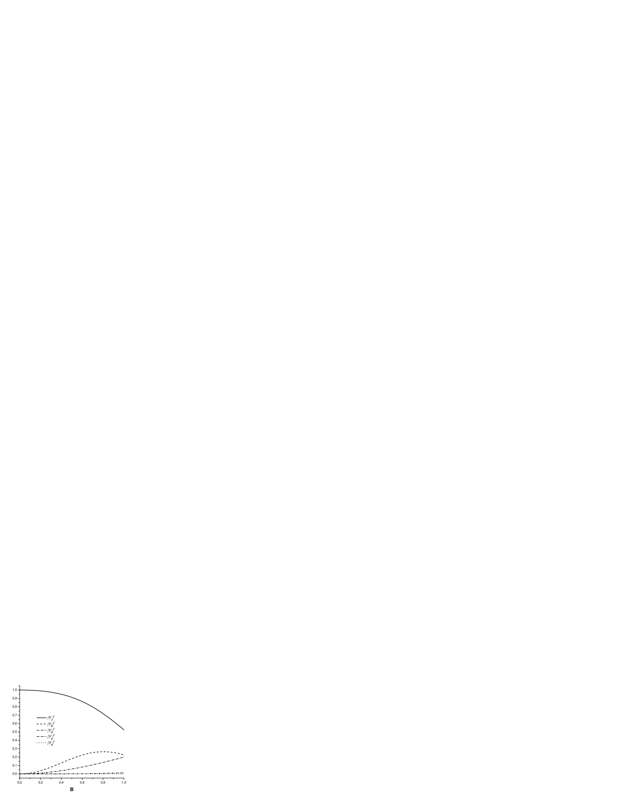
Figure 1: Relative intensities of spectral lines.

2) $\eta_{\bf k}T\ll 1$. In this limit it is valid to put $e^{-\eta_{\bf k}T}\sim 1$ in the expression for the intensity spectra to change it to

$$\begin{array}[]{c}\displaystyle{{I}_{\bf k}(t)=N^{2}G_{\bf k}^{2}e^{-\eta_{\bf k}t_{1}}}\displaystyle{\sum_{j=-\infty}^{\infty}2|Y_{j}|^{2}V(j)},\\ \displaystyle{V(m)=\frac{1-cos((\nu_{\bf k}+2mR)T)}{(\nu_{\bf k}+2mR)^{2}+\eta_{\bf k}^{2}/4}}.\end{array}$$ (78)

Over long times the spectrum of scattered light is now as well a collection of lines multiple to Rabi frequency with intensities proportional to $|Y_{j}|^{2}$. However, unlike the opposite case they are modulated with the frequency inverse to the pulse duration time. This modulation the line widths are of the order of inverse pulse duration time. For the central peak it is seen from the following expression :

$$\frac{1-cos(\nu_{\bf k}T)}{\nu_{\bf k}^{2}+\eta_{\bf k}^{2}/4}=\frac{\sum_{i=1}^{\infty}(-1)^{i-1}(\nu_{\bf k}T)^{2i}/(2i)!}{\nu_{\bf k}^{2}+\eta_{\bf k}^{2}/4}$$ (79)

for large values of $\nu_{\bf k}\gg\eta_{\bf k}$ the expression takes the form:

$$\frac{1-cos(\nu_{\bf k}T)}{\nu_{\bf k}^{2}+\eta_{\bf k}^{2}/4}\approx T^{2}/2!-\nu_{\bf k}^{2}T^{4}/4!+O(\nu_{\bf k}^{4}),$$ (80)

from which it follows that the line width value is of the order of $1/T$. Let us note that the intensity in the line center is always different from null. Indeed, at $\nu_{\bf k}\to 0$ we have:

$$\frac{1+e^{-\eta_{\bf k}T}-2e^{-\eta_{\bf k}T/2}cos(\nu_{\bf k}T)}{\nu_{\bf k}^{2}+\eta_{\bf k}^{2}/4}=T^{2}+O(T^{4})$$ (81)

IV Numerical modeling

In the previous section we obtained explicit expressions for intensity spectra of scattered radiation in case when parameter $B\ll 1$ which corresponds to the small density of atoms. This limitation was due to the method of successive approximations selected for our analysis. In case of large density values this method is not applicable. Thus, we have to solve the system of nonlinear system equations (39) using numerical methods.

In order to estimate the range of parameters where multicomponent spectra could be expected we introduced operators describing radiative and collisional relaxation.

$$\begin{array}[]{c}\displaystyle{\Gamma[{\rho^{a}}]=-i\gamma/2(|2\rangle\langle 2|{\rho^{a}}+{\rho^{a}}|2\rangle\langle 2|-2|1\rangle\langle 2|{\rho^{a}}|2\rangle\langle 1|),}\\ \displaystyle{\Gamma_{s}[{\rho^{a}}]=-i\gamma_{2}(|1\rangle\langle 2|{\rho_{12}^{a}}+|2\rangle\langle 1|{\rho_{21}^{a}})}.\\ \end{array}$$ (84)

Substituting these damping terms into the equations gives

$$\begin{array}[]{c}\displaystyle{i\frac{d{\rho^{a}}}{dt}}-[H_{a}+V_{a}+V_{a}^{p},{\rho^{a}}]-\Gamma[{\rho^{a}}]-\Gamma_{s}[{\rho^{a}}]=0,\\ \displaystyle{\frac{d\beta_{\bf k}^{{}^{\prime}}}{dt}=-(i\nu_{\bf k}+\eta_{\bf k}/2)\beta_{\bf k}^{{}^{\prime}}-\sum_{m}^{N}g_{m}({\bf k}_{\alpha})^{*}{\rho_{21}^{a}}},\\ \displaystyle{{I}_{\bf k}(t)=\eta_{\bf k}\hbar\omega_{\bf k}|\beta_{\bf k}^{{}^{\prime}}(t)|^{2}.}\end{array}$$ (88)

Also, we present the time integrated intensity spectra to make experimental verification of obtained results possible if such is to take place.

$$I_{\bf k}^{T}=\int_{0}^{\infty}{I}_{\bf k}(t)dt.$$ (89)

In ris. 2 one can see the intensity spectra of scattered light for a long compared to the mode dumping time pulse , $\eta_{\bf k}T\gg 1$, for different values of parameter $B$. For small values of $B$ in ris. 2(a) ot is seen that the ratios of line intensities generally meet the results reported in the previous section. The central peak with $\nu_{\bf k}=0$ is the only exception. This fact is explained by existence of residual radiation after the pulse has already passed the medium. With increasing value of $B$ the relative intensity of the central line grows substantially. The relative intensities of the side bands decrease while shifting to the center of the spectral range, see FIG 2(b),(c). Moreover, one can see that peaks multiple to 3 and 4 Rabi frequencies arise shifted significantly to the center. At extremely large densities $B\sim 1$ all components merge leaving the only central peak (FIG 2(d)).

Figure 2: Intensity spectrum of the scattered light $I_{\bf k}$ and time integrated spectrum $I_{\bf k}^{T}$, values of $I_{\bf k},I_{\bf k}^{T}$ are presented in relative units and proportional to $N^{2}$. $\Delta=0$,$R=10\pi$,$\gamma=0.01$, $\eta_{\bf k}=5$, $T=1.9$ $B=0.32,\;0.64,\;0.85,\;1.2$ for pictures (a,b,c,d) respectively.

The short pulse scattering, $\eta_{\bf k}T\ll 1$, is demonstrated in FIG 3 for different values of density. In FIG 3(a),(b) some additional peaks are well seen. These peaks arise due to modulations of the kind (80) for $6\pi$ and $10\pi$ pulses respectively. The general behavior of spectrum is just like the one displayed in the previous case, that is, the peaks shift toward the central line at $B\sim 1$ and finally merge.

Figure 3: Same as in FIG 2. $\Delta=0$,$R=10\pi$,$\gamma=0.01$, $\eta_{\bf k}=0.1$, picture (a) $T=0.3$, $B=0.28$, picture (b) $T=0.5$, $B=0.36$

The calculation carried out for different values of $\gamma,\gamma_{2}$showed that with shorter relaxation time the spectral picture is ”blurred”. At $\gamma,\gamma_{2}\sim 2/T$ the additional peaks induced by modulation practically vanish. However, the peaks multiple to $\pm 4R$ remain observable up until $\gamma_{2}T\sim 8$ (FIG 4).

Figure 4: Same as in FIG 2. $\Delta=0$,$R=10\pi$,$\gamma=0.5$,$\gamma_{2}=9$,$\eta_{\bf k}=1$, $T=1$, $B=0.74$

We examined the spectra as functions of detuning and found that the spectral pattern is very sensitive to the value of detuning. Even for $\Delta\sim~{}0.1R$ the spectrum is distorted showing increased intensities of the lines lying close to the excitation frequency. At $\Delta\sim~{}0.8R$ the multimode structure is no longer observed. The light is scattered at the frequency of the pulse.

V Summary

In this work we have carried out the analysis of scattering of a short laser pulse in a dense two-level medium. We used the approach based on the BBGKY-hierarchy for the reduced density operators. In the framework of the Hartree-Fock approximation and with use of the properties of coherent state operators we derived the cooperative field operator in the explicit form and compared our results with the well-known ones Bowden_79 . The transformations used in this work allowed us to derive the set of equations describing transient spectra of scattered light. The equations were analyzed using the method of successive approximations in the case when the medium was excited by a short rectangular laser pulse. A possibility was demonstrated to generate scattered light at frequencies multiple to Rabi frequency which is contributed by transient local field. The ratio of line intensities has been determined. We also demonstrated that additional satellites can occur in the spectrum due to modulation Rabi components as a result of finite pulse length.

In the final part of this work we carried out the numerical analysis of spectra. It was demonstrated that in the limit of small density the theoretical analysis well meets the results of calculations. However, for large densities, i.e., $B>0.3$ this theoretical approach becomes inapplicable. As the density is increased one can observe a significant shift of the satellites to the central line in came cases accompanied with generation of additional bands multiple to three and four Rabi frequencies.

Authors are grateful to A.N. Starostin for discussions and remarks received in the course of work. We would like to acknowledge the financial support from the Russian Foundation for Basic Research No.02-02-17153 and No.03-02-06590 and grants of the President of the Russian Federation No.MK1565.2003.02, No.MD338.2003.02 and No.NS1257.2003.02.

Appendix A. Cooperative field operator

In this section we will derive the explicit form for the cooperative field operator. Our attention is now for the expression (33):

$$\begin{array}[]{c}\displaystyle{[\tilde{V}_{af}^{p},\rho_{f}\rho_{a}]^{f}=\sum_{{\bf k}_{\alpha}}i}\displaystyle{[g_{l}({\bf k}_{\alpha})|2\rangle\langle 1|\beta_{\bf k}(t)^{{}^{\prime}}}-\\ -\displaystyle{g_{l}({\bf k}_{\alpha})^{*}|1\rangle\langle 2|\beta_{\bf k}^{{}^{\prime}*}(t),\rho_{f}{\rho^{a}}],}\\ \end{array}$$ (A.3)

where the equation for $\beta_{\bf k}(t)$ has the form:

$$\displaystyle{\frac{d\beta_{\bf k}^{{}^{\prime}}}{dt}=-(i\nu_{\bf k}+\eta_{\bf k}/2)\beta_{\bf k}^{{}^{\prime}}-\sum_{m}^{N}g_{m}({\bf k}_{\alpha})^{*}{\rho_{21}^{a}}}.$$ (A.4)

Solving the equation for $\beta_{\bf k}(t)^{{}^{\prime}}$ formally one can get:

$$\displaystyle{\beta_{\bf k}^{{}^{\prime}}(t)=-\sum_{l}^{N}g_{m}({\bf k}_{\alpha})^{*}\int_{0}^{t}{\rho_{21}^{a}}(\tau)e^{-i(\nu_{\bf k}+\eta_{\bf k}/2)(t-\tau)}d\tau}.$$ (A.6)

Now we substitute the result in (A.3) and by changing the summation over atomic and field variables for integration correspondingly over the volume and ${\bf k}$ come to

$$\begin{array}[]{c}\displaystyle{[\tilde{V}_{af}^{p},\rho_{f}\rho_{a}]^{f}=[R_{l}(t,{\bf r}_{l})|2\rangle\langle 1|-R_{l}^{*}(t,{\bf r}_{l})|1\rangle\langle 2|,\rho_{f}{\rho^{a}}]}\\ \displaystyle{R_{l}(t,{\bf r}_{l})=\int\int_{0}^{t}B_{lm}(kr_{lm})\times}\\ \displaystyle{\times{\rho_{21}^{a}}(\tau,{\bf r}_{m})e^{-i(\nu_{\bf k}+\eta_{\bf k}/2)(t-\tau)}d\tau}d{\bf r}_{m}k^{2}dk,\\ \end{array}$$ (A.10)

$$\begin{array}[]{c}\displaystyle{B_{lm}(kr_{lm})=\int\sum_{\alpha=\pm 1}g_{l}({\bf k}_{\alpha})g_{m}({\bf k}_{\alpha})^{*}d\Omega,}\end{array}$$ (A.12)

where $d\Omega$ is the spatial angle element, $k=|{\bf k}|$, $r_{lm}=|{\bf r}_{l}-{\bf r}_{m}|$. Integral of the kind (A.12) have been considered in Knight and are representable in the following form:

$$\begin{array}[]{c}\displaystyle{B_{ml}(x)=\frac{2\pi\omega_{\bf k}||{\mu}_{21}||^{2}}{\hbar W}}\times\\ \times\displaystyle{\Biggl{(}b\frac{sin(x)}{x}+c\Bigl{(}\frac{sin(x)}{(x)^{3}}-\frac{cos(x)}{(x)^{2}}\Bigr{)}\Biggr{)}}.\\ \end{array}$$ (A.15)

Transition constants $b,c$ for various polarizations $\Delta M$ are

$$\begin{array}[]{c}\displaystyle{\Delta M=0:\;\;\;\;\;b=0,c=2,}\\ \displaystyle{\Delta M=\pm 1:\;\;\;\;\;b=1,c=-1.}\\ \end{array}$$ (A.18)

With use of (A.15) the integral (A.10) was examined in Bowden , where allowing for disregard of signal retardation they obtained the cooperative field operator:

$$V_{a}^{p}=\displaystyle{-i\frac{3n({\bf r})G\lambda_{21}^{3}}{8\pi^{2}}\gamma/2\;|2\rangle\langle 1|{\rho_{21}^{a}}(t,{\bf r}_{l})+H.c.,}$$ (A.19)

where $\gamma=\displaystyle{\frac{4\omega_{21}^{3}||\mu_{21}||^{2}}{3\hbar c^{3}}}$ is the spontaneous decay rate from the upper state, $n({\bf r})$ is the density of the sample, and $G$ represents the geometrical factor being a function of selected geometry of the sample, its dimensions, and polarization of scattered light.

References

• (1)
• (2) Weisskopf V., Wigner E. Z.Phys. , 63, 54 (1930); Weisskopf V. Ann. Phys. Leipzig, 9, 23 (1931).
• (3) Mollow B.R. Phys. Rev., 188, 1969 (1969).
• (4) Schuda F., Stroud Jr. C.R., Hercher M.J. Phys. B, 7, L198 (1974); Harting W., Rasmussen W., Schieder R., Walther H. Z. Phys. A., 278, 205 (1976); Wu F.Y., Crove R.E., Ezekiel S. Phys. Rev. A 15, 227, (1977).
• (5) Dicke R.H. Phys. Rev. 93, 99 (1954).
• (6) A. V. Andreev, V.I. Emelyanov,and Yu. A. Ilinskii, Cooperative Effects in Optics, edited by E. R. Pike, Malvern Physics Series (IOP Publishing, London, 1993).
• (7) C. M. Bowden and C. Sung, Phys. Rev. A 19, 2392 (1979);
• (8) F. A. Hopf, C. M. Bowden, and W. H. Louisell, Phys. Rev. A 29, 2591 (1984); Ben-Aryeh and C. M. Bowden, Opt. Commun. 59, 224 (1986); C.M. Bowden, J.P. Dowling,Phys. Rev. A 47, 1247 (1993); Phys. Rev. A 47, 1514 (1993).
• (9) M.E. Crenshaw, C.M. Bowden, Phys. Rev. A 53 1139 (1996).
• (10) T. M. Bowden and M. E. Crenshaw, Opt. Commun. 179, 63 (2000).
• (11) M.P. Hehlen, H. U. G del, Q. Shu, J. Rai, S. Rai, and S. C. Rand, Phys. Rev. Lett. 73, 1103 (1994); M. P. Hehlen, H. U. G del, Q. Shu, and S. C. Rand, J. Chem. Phys. 104, 1232 (1996); S. R. L thi, M. P. Hehlen, T. Riedener, and H. U. G del, J. Lumin. 76 77, 447 (1998); M.P. Hehlen, A. Kuditcher, S. C. Rand, and S. R. L thi, Phys. Rev. Lett. 82, 3050 (1999).
• (12) Kuditcher, M. P. Hehlen, C. M. Florea, K. W. Winick, and S. C. Rand, Phys. Rev. Lett. 84, 1898 (2000).
• (13) M.E. Crenshaw and C.M. Bowden, Phys. Rev. A 63, 013801 (2000); M.E. Crenshaw and C.M. Bowden, Phys. Rev. Lett. 85, 1851 (2000).
• (14) M. Fleischhauer, Phys. Rev. A 60, 2534 (1999).
• (15) S. Scheel, L. Kn ll, D.-G. Welsch, and S. M. Barnett, Phys. Rev. A 60, 1590 (1999); S. Scheel, L. Kn ll, and D.-G. Welsch, Phys. Rev. A 60, 4094 (1999).
• (16) R. Friedberg, S.R. Hartmann, and J.T. Manassah, Phys. Rev. A 40, 2446 (1989).
• (17) J.T. Manassah, Opt. Commun. 191, 435, (2001);
• (18) G. S. Agarwal, A. C. Brown, L. M. Narducci and G. Vetri, Phys. Rev. A 15, 1613 (1977).
• (19) A. S. J. Amin and J. G. Cordes, Phys. Rev.A 18, 1298 (1978).
• (20) I. R. Senitzky, Phys. Rev. Lett. 40, 1334 (1978).
• (21) H. J. Carmichael, Phys. Rev. Lett. 43, 1106 (1979).
• (22) G. S. Agarwal, R. Saxena, L. M. Narducci, D. H. Feng and R. Gilmore, Phys. Rev. A 21, 257 (1980).
• (23) P. D. Drummond and S. S. Hassan, Phys. Rev. A 22, 662 (1980).
• (24) H. S. Freedhoff, Phys. Rev. A 19, 1132 (1979).
• (25) Z. Ficek, R. Tanas and S. Kielich, Opt. Commun. 36, 121 (1981)
• (26) S. J. Kilin, J. Phys. B 13, 2653 (1980)
• (27) M. Kus and K. Wodkiewicz, Phys. Rev. A 23, 853 (1981).
• (28) R. D. Griffin and S. M. Harris, Phys. Rev. A 25, 1528 (1982).
• (29) Z. Ficek, R. Tanas and S. Kielich, J. Phys. B 17, 1491 (1984).
• (30) L. Mandel, E. Wolf, ”Optical Coherence and Quantum Optics”, Cambrige University Press (1995);.
• (31) A.A.Pantelev, Vl.C.Roerich, A.N.Starostin, JETP, 96, 222 (2003).; Vl.C.Roerich, M.G.Gladush, ”Progress in Nonequilibrium Green’s Functions II”, M. Bonitz and D. Semkat (eds.), World Scientific Publ., Singapore (2003).
• (32) Bonitz M. Quantum Kinetic Theory. B.G.Teubner Stuttgart-Leipzig (1998).
• (33) A.M. Perelomov ”Generalized Coherent States and Their Applications”, Springer, Berlin(1986).
• (34) Y. Ben-Aryeh, C.M. Bowden, J.C. Englund; Phys.Rev. A 34, 3917 (1986).
• (35) I. S. Gradshteyn and I. M. Ryzhik, Table of Integrals, Series and Products (Academic Press, New York, 1980), p. 1034
• (36) P.W. Milloni, P.L. Knight, Phys. Rev. A 4, 1096 (1974).