Revivals of Coherence in Chaotic Atom-Optics Billiards

Abstract

We investigate the coherence properties of thermal atoms confined in optical dipole traps where the underlying classical dynamics is chaotic. A perturbative expression derived for the coherence of the echo scheme of [Andersen et. al., Phys. Rev. Lett. 90, 023001 (2003)] shows it is a function of the survival probability or fidelity of eigenstates of the motion of the atoms in the trap. The echo coherence and the survival probability display ”system specific” features, even when the underlying classical dynamics is chaotic. In particular, partial revivals in the echo signal and the survival probability are found for a small shift of the potential. Next, a ”semi-classical” expression for the averaged echo signal is presented and used to calculate the echo signal for atoms in a light sheet wedge billiard. Revivals in the echo coherence are found in this system, indicating they may be a generic feature of dipole traps.

I Introduction

The capability to control and manipulate quantum systems that has been developed in recent years holds promise for applying quantum systems to information processing [1]. This possible application has drawn much attention to the subject of decoherence/dephasing, where the concept of ”fidelity” and ”survival probability” plays a major role. Some of the possible quantum information schemes involve superposition states of the internal states of trapped neutral atoms or ions. Interaction with the trapping potential often causes these superposition states to dephase, but, in analogy with the spin echo [2], a coherence ”echo” can be used to preserve the coherence [3] [4] [5]. Under certain conditions the echo coherence of trapped atoms is limited by the quantum dynamics of the atoms in the trap, thereby enabling study of quantum dynamics by echo techniques, but also stressing that the quantum dynamics of the atoms in the trap is of great importance to the coherence of their internal states [4].

In this paper the dephasing of trapped atoms in coherent superposition states of their internal states is investigated. A special focus is put on neutral atoms trapped in optical dipole traps, where the underlying classical dynamics is chaotic namely atom-optics billiards [6][7]. This is done partly because chaotic billiards where used in the past as a simplified model to describe decoherence [8], and partly because they can have very long coherence times [9]. The atoms are considered ”hot”, meaning that their temperature is much larger than the mean level spacing of the trap, so they occupy high excited states in the trap, and an output of the experiment is an ensemble average over many occupied states.

The strength of the dipole potential depends on the internal state of the atom. This causes atoms initially in coherent superposition states of their internal degree of freedom but with different external initial conditions to acquire different phases thereby loosing the macroscopic coherence. This dephasing can be suppressed by echo techniques, where each part of the superposition state spends an equal amount of time in each potential, thereby ensuring that the phases acquired are equal [4][5]. However, since the external potentials are slightly different (we denote this difference ”the perturbation”), also the dynamics depends on the internal state, and loss of coherence from this is not cancelled by echo techniques. For far-off -resonance optical dipole traps such a perturbation is small, so a perturbative result is of great interest. In section III a perturbative expression for the echo signal is derived, and confirmed numerically, showing that the echo signal can be written as a function of the survival probability or fidelity of eigenstates of the motion of the atoms in the trap. Based on this perturbative result the long-time echo coherence of atomic ensembles is predicted.

In the perturbative limit the echo coherence and the survival probability display ”system specific” features, despite the fact that the underlying classical dynamics is ergodic[10]. This is demonstrated in section IV by showing partial revivals in the echo signal and the survival probability for a perturbation consisting of a small spacial shift of the potential. In section V a ”semiclassical” perturbative expression for the averaged echo coherence is derived. Two billiard systems are considered throughout the paper. First, an ”idealized” system - a shift perturbation of the hard-wall Bunimovich billiard [12] where eigenstates can be computed efficiently [13] is used to confirm the validity of the perturbative and semiclassical approximations by comparing them to a full quantum calculation (sections IV and V). These approximations are then used in section VI to calculate the echo coherence for micro wave (MW) spectroscopy of atoms in an experimental realizable atom optics billiard, namely the light-sheet wedge billiard [6] [14], where revivals in analogy with those in the hard-wall stadium are found. This suggest that revivals of coherence may be a generic feature of optical dipole traps.

II Micro Wave Spectroscopy and Quantum Dynamics of trapped Atoms

In this section pulsed micro wave spectroscopy on optical trapped alkali atoms is considered.

The ground state of alkali atoms contains two hyperfine states with an energy splitting of $E_{HF}=\hbar\omega_{HF}$, each containing several magnetic substates. The hyperfine energy splitting in Caesium atoms is the foundation of modern time scales, so MW spectroscopy of this transition in an isolated environment is of great importance and is therefore a very advanced field. However, many quantum information processing schemes require trapped atoms or ions, and if neutral alkali atoms are placed inside an optical trapping potential, then the energy levels are changed. Since the optical dipole potential is inversely proportional to the detuning of the trap laser from resonance [15] and the detuning will differ by the hyperfine splitting, then there is a slight difference in potential for atoms in different hyperfine states, even if the states considered have the same matrix element for the dipole interaction with the trapping light. For such two states (denoted $\left|\uparrow\right\rangle$ and $\left|\downarrow\right\rangle$) the Hamiltonian considered can be written as,

$$H=H_{\downarrow}\left|\downarrow\right\rangle\left\langle\downarrow\right|+\left(H_{\uparrow}+E_{HF}\right)\left|\uparrow\right\rangle\left\langle\uparrow\right|=\left(\frac{p^{2}}{2m}+V_{\downarrow}\left({\bf x}\right)\right)\left|\downarrow\right\rangle\left\langle\downarrow\right|+\left(\frac{p^{2}}{2m}+V_{\uparrow}\left({\bf x}\right)+E_{HF}\right)\left|\uparrow\right\rangle\left\langle\uparrow\right|,$$ (1)

where $p$ is the atomic center of mass momentum and $V_{\downarrow}$ [$V_{\uparrow}$] the external potential for an atom in state $\left|\downarrow\right\rangle$ [$\left|\uparrow\right\rangle$]. Typically $V$ is much smaller than $E_{HF}$ and $\left(V_{\uparrow}-V_{\downarrow}\right)/V_{\downarrow}\sim 10^{-3}-10^{-5}$ [4][5]. The eigenenergies of this Hamiltonian consist of two manifolds (belonging to $\left|\downarrow\right\rangle$ and $\left|\uparrow\right\rangle$) separated in energy by $E_{HF}$ (see Fig. 1).

The initial step in MW spectroscopy is to prepare all the atoms in one of the spin states involved ($\left|\downarrow\right\rangle$), so their total wave function can be written as $\left|\downarrow\right\rangle\otimes\left|\psi_{i}\right\rangle\equiv\left|\downarrow,\psi_{i}\right\rangle$, where $\left|\psi_{i}\right\rangle$ represents the motional (external degree of freedom) part of their wave function. If atoms prepared in $\left|\downarrow,\psi_{i}\right\rangle$ are irradiated with a MW field close to resonance with $\omega_{HF}$, then transitions between eigenstates belonging to different manifolds can be driven. The matrix elements for these transitions is given by $C_{nk}=\left\langle k_{\uparrow}\mid n_{\downarrow}\right\rangle\times M_{\downarrow\rightarrow\uparrow}$ where $M_{\downarrow\rightarrow\uparrow}$ is the free space matrix element for the internal state transition, and $\left\langle k_{\uparrow}\mid n_{\downarrow}\right\rangle$ is the overlap between $\left|n_{\downarrow}\right\rangle$, the initial eigenstate of $H_{\downarrow}$, and $\left|k_{\uparrow}\right\rangle$, the final eigenstate of $H_{\uparrow}$ (here the very small momentum of the MW photon is neglected). Since in general each of the eigenstates in the $\left|\downarrow\right\rangle$-manifold is coupled to many eigenstates in the $\left|\uparrow\right\rangle$-manifold by the MW-field, there is no simple prediction of the wave function after MW irradiation. However, in the simple limit of very short MW-pulses the external wave function is left unchanged and only the internal state of the atom is changed. Such a short pulse that puts atoms initially in $\left|\downarrow,\psi_{i}\right\rangle$, into the coherent superposition state $\frac{1}{\sqrt{2}}\left|\downarrow,\psi_{i}\right\rangle+\frac{i}{\sqrt{2}}\left|\uparrow,\psi_{i}\right\rangle$ is called a $\frac{\pi}{2}$-pulse and a pulse that flips the spin to $i\left|\uparrow,\psi_{i}\right\rangle$ is called a $\pi$-pulse.

In the widely used Ramsey spectroscopy technique [16], atoms initially prepared in $\left|\downarrow,\psi_{i}\right\rangle$ (assumed to be a pure state) and irradiated with a $\frac{\pi}{2}$-pulse to generate the wave function $\frac{1}{\sqrt{2}}\left|\downarrow,\psi_{i}\right\rangle+\frac{i}{\sqrt{2}}\left|\uparrow,\psi_{i}\right\rangle$. After some time $\tau$ this state will, in the rotating frame of the MW field, evolve into $\frac{1}{\sqrt{2}}\exp\left(-i\frac{H_{\downarrow}}{\hbar}\tau\right)\left|\downarrow,\psi_{i}\right\rangle+\frac{i}{\sqrt{2}}\exp\left(-i\left(\frac{H_{\uparrow}}{\hbar}+\Delta\right)\tau\right)\left|\uparrow,\psi_{i}\right\rangle$, where $\Delta=\omega_{HF}-\omega_{MW}$ is the MW-detuning. Then the atoms are irradiated with a second $\frac{\pi}{2}$-pulse generating the wave function $\frac{1}{2}\left(\exp\left(-i\frac{H_{\downarrow}}{\hbar}\tau\right)-\exp\left(-i\left(\frac{H_{\uparrow}}{\hbar}+\Delta\right)\tau\right)\right)\left|\downarrow,\psi_{i}\right\rangle+\frac{i}{2}\left(\exp\left(-i\left(\frac{H_{\uparrow}}{\hbar}+\Delta\right)\tau\right)+\exp\left(-i\frac{H_{\downarrow}}{\hbar}\tau\right)\right)\left|\uparrow,\psi_{i}\right\rangle$. The population of state $\left|\uparrow\right\rangle$ is then,

$$P_{\uparrow}=\frac{1}{2}\left(1+\left|\left\langle\psi_{i}\left|e^{i\left(\frac{H_{\downarrow}}{\hbar}\right)\tau}e^{-i\left(\frac{H_{\uparrow}}{\hbar}\right)\tau}\right|\psi_{i}\right\rangle\right|\cos\left(\Delta\tau+\phi_{i}\left(\tau\right)\right)\right),$$ (2)

where $\phi_{i}\left(\tau\right)$ is a phase depending on the initial state $\left|\psi_{i}\right\rangle$ and the dynamics of it in the trap. By choosing $\Delta$ sufficiently large, compared to variations in $\phi_{i}\left(\tau\right)$ Eq. 2 yields the well known cosinusodial Ramsey-fringes as a function of $\Delta\tau$, but with a fringe contrast reduced to the square root of the fidelity of the external motion in the trap $P_{FID}\equiv\left|\left\langle\psi_{i}\left|e^{i\left(\frac{H_{\downarrow}}{\hbar}\right)\tau}e^{-i\left(\frac{H_{\uparrow}}{\hbar}\right)\tau}\right|\psi_{i}\right\rangle\right|^{2}$. In the case where $\left|\psi_{i}\right\rangle$ is an eigenstate of $H_{\downarrow}$, the fidelity can be written $P_{FID}=\left|\left\langle\psi_{i}\left|e^{-i\left(\frac{H_{\uparrow}}{\hbar}\right)\tau}\right|\psi_{i}\right\rangle\right|^{2}\equiv P_{SRV}$ and is therefore often denoted the survival probability of $\left|\psi_{i}\right\rangle$ in $H_{\uparrow}$. Because the fidelity shows up in many such simple experiments, especially in connection to quantum information processing schemes where it measures the overlap between the desired state $e^{-i\left(\frac{H_{d}}{\hbar}\right)\tau}\left|\psi_{i}\right\rangle$ and the actual state $e^{-i\left(\frac{H_{a}}{\hbar}\right)\tau}\left|\psi_{i}\right\rangle$, and because it can be used as an indicator of quantum chaos, its decay have been an immensely studied topic throughout [17].

However, experiments are often not performed with atoms initially prepared in a pure initial state $\left|\psi_{i}\right\rangle$, but with atoms in a thermal mixture of states. Since $\phi_{i}\left(\tau\right)$ depends on the initial state, then the fringe contrast in a Ramsey experiment will decay rapidly, not due to a decay in the fidelity of the individual states thermally populated, but because the cosine terms from different populated states get out of phase [4]. This rapid loss of coherence is a problem in quantum information schemes [5] and prevents the use of Ramsey spectroscopy for studying quantum dynamics [4]. The loss in coherence may be overcome by adding an additional potential making $H_{\uparrow}=H_{\downarrow}$, and thereby decoupling the external dynamics from the spectroscopic evolution [18]. This is however not always possible and does not enable the use of MW-spectroscopy for dynamical studies. The echo pulse sequence demonstrated in [3][4][5] provides a more general solution to suppress the inhomogeneous dephasing of superposition states.

The echo pulse sequence consists of three short pulses ($\frac{\pi}{2}-\pi-\frac{\pi}{2}$), separated by two dark periods of equal duration $\tau$, after which the population of $\left|\uparrow\right\rangle$ is measured. In analogy to Eq. 2 the population of state $\left|\uparrow\right\rangle$ can be written as:

$$P_{\uparrow}=\frac{1}{2}\left[1-\mathop{\rm Re}\left(\left\langle\psi_{i}\left|e^{i\left(\frac{H_{\downarrow}}{\hbar}\right)\tau}e^{i\left(\frac{H_{\uparrow}}{\hbar}\right)\tau}e^{-i\left(\frac{H_{\downarrow}}{\hbar}\right)\tau}e^{-i\left(\frac{H_{\uparrow}}{\hbar}\right)\tau}\right|\psi_{i}\right\rangle\right)\right]$$ (3)

In the following we denote the quantity $F_{ECH}=\left\langle\psi_{i}\left|e^{i\left(\frac{H_{\downarrow}}{\hbar}\right)\tau}e^{i\left(\frac{H_{\uparrow}}{\hbar}\right)\tau}e^{-i\left(\frac{H_{\downarrow}}{\hbar}\right)\tau}e^{-i\left(\frac{H_{\uparrow}}{\hbar}\right)\tau}\right|\psi_{i}\right\rangle$ the ”echo amplitude”. $F_{ECH}=1$ indicates complete preservation of coherence and yields $P_{\uparrow}=0$, whereas $F_{ECH}=0$, yielding $P_{\uparrow}=\frac{1}{2}$ indicates complete loss of coherence [19]. From Eq. 3 it is seen that the echo amplitude is insensitive to the addition of constants to $H_{\uparrow}$ and $H_{\downarrow}$, so in contrary to the Ramsey signal (Eq. 2) $P_{\uparrow}$ of Eq. 3 does not depend on $\omega_{MW}$ and $E_{HF}$, but only on the quantum dynamics of the atoms in the potentials. The rapid loss of coherence when a thermal mixtures of states is considered has vanished, making echo techniques of interest in experiments on quantum information processing [5]. This also means that even for thermal mixtures of states echo spectroscopy can yield information on the quantum dynamics of the trapped atoms, as was demonstrated in [4] for more than $10^{6}$ thermally populated states.

III The Connection Between the Echo and the Survival Amplitudes and long time behavior.

In this section a second order perturbative expression for the echo amplitude of an eigenstate is derived, showing that it can be written as a function of the fidelity or survival amplitude, thereby also predicting the time average of the echo amplitude.

Since thermal atoms can be considered as a mixture of eigenstates, the attention is now turned to the echo amplitude of an eigenstate of $H_{\downarrow}$. The echo amplitude of an eigenstate $\left|m_{\downarrow}\right\rangle$ of $H_{\downarrow}$ can be rewritten:

$$F_{ECH}\left(\left|m_{\downarrow}\right\rangle,\tau\right)=\sum_{l,k,n}\exp\left(i\left(\omega_{m}^{\downarrow}+\omega_{l}^{\uparrow}-\omega_{k}^{\downarrow}-\omega_{n}^{\uparrow}\right)\tau\right)\left\langle m_{\downarrow}\mid l_{\uparrow}\right\rangle\left\langle l_{\uparrow}\mid k_{\downarrow}\right\rangle\left\langle k_{\downarrow}\mid n_{\uparrow}\right\rangle\left\langle n_{\uparrow}\mid m_{\downarrow}\right\rangle$$ (4)

Since adding constants to $H_{\uparrow}$ and $H_{\downarrow}$ does not change the echo we can without loss of generality set $\omega_{m}^{\uparrow}=\omega_{m}^{\downarrow}=0$. Now for atoms trapped in far off resonance optical dipole traps made of linearly polarized light the difference between $H_{\uparrow}$ and $H_{\downarrow}$ is very small, so a perturbative result is of great interest. For a small perturbation $\left\langle n_{\uparrow}\mid n_{\downarrow}\right\rangle\simeq 1-\epsilon_{n}^{2}$ and $\left\langle k_{\uparrow}\mid n_{\downarrow}\right\rangle$ is of the order $\epsilon$ or less. Rewriting Eq. 4 and keeping only terms up to order $\epsilon^{2}$ yields:

$$F_{ECH}\left(\left|m_{\downarrow}\right\rangle,\tau\right) \simeq 2\sum_{n\neq m}\exp\left(-i\omega_{n}^{\uparrow}\tau\right)\left|\left\langle n_{\uparrow}\mid m_{\downarrow}\right\rangle\right|^{2}+$$ (10)

$$\sum_{n\neq m}\exp\left(-i\omega_{n}^{\downarrow}\tau\right)\left|\left\langle n_{\downarrow}\mid m_{\uparrow}\right\rangle\right|^{2}+$$

$$\sum_{n\neq m}\exp\left(i\omega_{n}^{\uparrow}\tau\right)\left|\left\langle n_{\uparrow}\mid m_{\downarrow}\right\rangle\right|^{2}-$$

$$\sum_{n\neq m}\exp\left(i\left(\omega_{n}^{\uparrow}-\omega_{n}^{\downarrow}\right)\tau\right)\left|\left\langle n_{\uparrow}\mid m_{\downarrow}\right\rangle\right|^{2}-$$

$$\sum_{n\neq m}\exp\left(-i\left(\omega_{n}^{\uparrow}+\omega_{n}^{\downarrow}\right)\tau\right)\left|\left\langle n_{\uparrow}\mid m_{\downarrow}\right\rangle\right|^{2}+$$

$$\left|\left\langle m_{\uparrow}\mid m_{\downarrow}\right\rangle\right|^{4}$$

This rewriting does not look like a simplification of Eq. 4, but first it is noted that the echo is no longer a function of   matrix elements like $\left\langle n_{\uparrow}\mid m_{\downarrow}\right\rangle$ but only a of their absolute value square, often referred to as the local density of states (LDOS) [10]. Second, note that since $\omega_{m}^{\uparrow}=\omega_{m}^{\downarrow}=0$, then typically $\omega_{n}^{\uparrow}-\omega_{n}^{\downarrow}<<\omega_{n}^{\downarrow}$, so except for extreme long times the approximation $\omega_{n}^{\uparrow}\simeq\omega_{n}^{\downarrow}\equiv\omega_{n}$ can be used. For high excited states $\sum_{n\neq m}\exp\left(i\left(\omega_{n}^{\uparrow}\right)\tau\right)\left|\left\langle n_{\uparrow}\mid m_{\downarrow}\right\rangle\right|^{2}=\sum_{n\neq m}\exp\left(-i\left(\omega_{n}^{\uparrow}\right)\tau\right)\left|\left\langle n_{\uparrow}\mid m_{\downarrow}\right\rangle\right|^{2}$ is also a good approximation, for times much shorter than $1/\Delta_{mls}$ with $\Delta_{mls}$ the mean level spacing. Using these approximations Eq. 10 can be rewritten as:

$$F_{ECH}\left(\left|m_{\downarrow}\right\rangle,\tau\right) \simeq 4\sum_{n\neq m}\exp\left(-i\omega_{n}\tau\right)\left|\left\langle n_{\uparrow}\mid m_{\downarrow}\right\rangle\right|^{2}-$$ (13)

$$\sum_{n\neq m}\exp\left(-2i\omega_{n}\tau\right)\left|\left\langle n_{\uparrow}\mid m_{\downarrow}\right\rangle\right|^{2}+$$

$$\left|\left\langle m_{\uparrow}\mid m_{\downarrow}\right\rangle\right|^{6},$$

where $\left|\left\langle m_{\uparrow}\mid m_{\downarrow}\right\rangle\right|^{6}\simeq 1-6\epsilon_{m}^{2}$. The quantity $\left\langle m_{\downarrow}\left|\exp\left(-i\left(\frac{H_{\uparrow}}{\hbar}-\omega_{m}^{\uparrow}\right)\tau\right)\right|m_{\downarrow}\right\rangle$ is denoted the survival amplitude ($F_{SRV}$), since its length square is the survival probability. Writing the survival amplitude in the same way as Eq. 13 shows that Eq. 13 yields a simple relation between the echo amplitude and the survival amplitude of an eigenstate in the perturbative limit:

$$F_{ECH}\left(\left|m_{\downarrow}\right\rangle,\tau\right) \simeq 4F_{SRV}\left(\left|m_{\downarrow}\right\rangle,\tau\right)-F_{SRV}\left(\left|m_{\downarrow}\right\rangle,2\tau\right)-2$$ (14)

Eq. 14 indicates that the time average of the echo amplitude is always smaller than the time average of the survival amplitude. Hence in the low temperature regime, where the decay of coherence is set by the decay of the survival amplitude, and not by the thermal spread of initial conditions, a Ramsey type experiment will yield better coherence than an echo experiment (see Eq. 2). This is in agreement with the experimental results published in [3].

From Eq. 13 it is seen that for times $\tau$ where the approximation $\omega_{n}^{\uparrow}\simeq\omega_{n}^{\downarrow}$ is valid, the constant contribution to the echo signal is not given by the infinite long time limit $\left|\left\langle m_{\uparrow}\mid m_{\downarrow}\right\rangle\right|^{4}$ but by $\left|\left\langle m_{\uparrow}\mid m_{\downarrow}\right\rangle\right|^{6}$. This is a rather peculiar result since $\left|\left\langle m_{\uparrow}\mid m_{\downarrow}\right\rangle\right|^{6}<\left|\left\langle m_{\uparrow}\mid m_{\downarrow}\right\rangle\right|^{4}$ hence it implies that waiting for dephasing to occur on time scales of $1/\left(\omega_{n}^{\uparrow}-\omega_{n}^{\downarrow}\right)$ will increase the ensemble average of the echo coherence. For perturbations that conserve the eigenspectrum the $\left|\left\langle m_{\uparrow}\mid m_{\downarrow}\right\rangle\right|^{6}$ echo level persists for all times.

In [4] we compared the measured long time echo signal for atoms confined in a Gaussian laser beam to a calculation based on the ensemble average of the infinite time level of $\left|\left\langle m_{\uparrow}\mid m_{\downarrow}\right\rangle\right|^{4}$. However, approximating the Gaussian trap of [4] by a harmonic oscillator yields that typically $2\pi/\left(\omega_{n}^{\uparrow}-\omega_{n}^{\downarrow}\right)\sim 5s$, whereas the long time echo level was measured when the initial oscillations had died out, typically after $\tau\sim 10ms$. Hence, from the perturbative treatment we expect to observe the ensemble averaged $\left|\left\langle m_{\uparrow}\mid m_{\downarrow}\right\rangle\right|^{6}$ echo level rather than the $\left|\left\langle m_{\uparrow}\mid m_{\downarrow}\right\rangle\right|^{4}$ level. We repeated the echo-level calculation of [4] using now the assumption that the long time echo signal is given by $\left|\left\langle m_{\uparrow}\mid m_{\downarrow}\right\rangle\right|^{6}$, and found better agreement with the experimental data published in [4] as compared to the $\left|\left\langle m_{\uparrow}\mid m_{\downarrow}\right\rangle\right|^{4}$ calculation, but due to the uncertainty of the data points no definitive conclusion can be made [11].

Finally, the simplified model presented here predicts that if $\left|\left\langle m_{\uparrow}\mid m_{\downarrow}\right\rangle\right|^{6}\simeq 1$ for all occupied states, then perfect echo coherence will persist for infinite times. In real systems, there are effects, such as photon scattering or temporal fluctuations in the trap depth not taken into account in our model (Eq. 1) causing echo coherence to be lost on long time scales [4] [5].

IV Equation 7, and Decay and Revivals of Echo and Survival Probability.

In this section the validity of Eq. 14 and the behavior of the quantities involved in it, are investigated by numerical calculations on a chaotic hard wall Burnimovich stadium [12]. This system is used as a test system, since the Burnimovich stadium has become almost a synonym with classical chaotic billiard dynamics, and since the scaling method of [13][20] enables efficient computation of high excited eigenstates of this system. It is demonstrated that the echo amplitude and the survival probability show partial revivals at certain times for a spacial shift perturbation.

The stadium considered consists of two semicircles of radius 1, connected by two lines of length 2 (see fig. 2). We consider the perturbation caused by shifting $V_{\uparrow}\left({\bf x}\right)$ a small amount along the long axis of the stadium compared to $V_{\downarrow}\left({\bf x}\right)$. This perturbation conserves the eigenspectrum so $\omega_{n}^{\uparrow}=\omega_{n}^{\downarrow}$. The shift also has direct relevance to the ”dephasing free” atom optics billiard proposed in [9], and illustrates some of the points of later sections.

The computation of the echo and the survival probability is done in the straight forward way. A large cluster containing $\sim 1300$ eigenstates with energies around 11000 is computed using the scaling method of [13]. The units h  =2m=1 are used so the eigenstates in the interior of the billiard are solutions to $\nabla^{2}\left|\psi\right\rangle=-k^{2}\left|\psi\right\rangle$ and are vanishing on the boundary. The transformation matrix $T$ taking states from a representation in eigenstates of  $H_{\uparrow}$ to a representation in eigenstates of $H_{\downarrow}$ is then computed by computing the overlap integral of the eigenstates of $H_{\uparrow}$ with those of $H_{\downarrow}$ (the length square of the elements of $T$ being the LDOS [10]). The computation of the overlaps is efficiently done using the methods of [20]. Since the time evolution of a state in the representation of eigenstates of the Hamiltonian under which it evolves is trivial, it is a trivial task to compute the echo and the survival amplitude when $T$ is known using Eq. 14. The issue of $T$ not being completely unitary for a hard wall billiard is addressed in [10].

The structure of $T$ can depend on the perturbation even when the underlying classical dynamics is chaotic [10][20] [21]. In Fig. 3 a plot of the square of the elements of $T$ is shown for the perturbation of a shift of 0.004, where two distinct sidebands are seen. This structure induces special behavior of the echo and the survival probability, since an eigenstate of $H_{\downarrow}$ will show a (partial) revival when evolved in $H_{\uparrow}$ at the time the sidebands have acquired a phase of 2$\pi$. This is demonstrated in Fig 4, where the echo and survival probability for several different eigenstates are shown. They all show revivals at the time $\tau_{R}$ corresponding to the sidebands acquiring a phase of 2$\pi.$ At longer times the revivals from different states get out of phase due to the finite width of the sidebands in Fig. 3. We note that the revivals seen in Fig. 4 are not the trivial revivals originating from the system being discrete, but they appears since the nature of the difference between $H_{\downarrow}$ and $H_{\uparrow}$ induces ”selection rules” that determines to which states in $H_{\uparrow}$ an eigenstate of $H_{\downarrow}$ is coupled.

Shown in Fig. 5 is the perturbative approximation Eq. 14 to the echo, together with the exact calculations for a shift of 0.001 (Fig. 5a) and 0.008 (Fig. 5b), showing good agreement, even for large perturbations. In 5c the RMS deviation between the echo and the approximation (Eq. 14) for the time interval 0-0.1 is shown as a function of the shift. It is seen that the deviation grows as $\epsilon^{3}$, as expected from Eq. 14 being a second order approximation to the echo. This indicates that the other approximations made are valid.

In Fig. 6 the difference between the exact echo and the approximation (Eq. 14) is shown, for long times, for one of the states of Fig. 4. No divergence as a function of time is observed. This is subscribed to the fact that the terms neglected in order to obtain Eq. 14 are oscillatory in time.

V Semi-Classical Estimation of the Echo Amplitude

In this section the echo amplitude of an ensemble of high excited eigenstates is calculated using classical estimations of the LDOS [10]. The method is confirmed by comparison to a full quantum calculation on a hard-wall Burnimovich stadium. It is then used in section VI to calculate the echo in a chaotic atom optics billiard, that have been demonstrated experimentally in the past [6][14]. Revivals in analogy with those of the previous section are found to appear.

From the fact that the perturbative limit is considered so $\overline{\left|\left\langle m_{\uparrow}\mid m_{\downarrow}\right\rangle\right|^{6}}\simeq\overline{\left|\left\langle m_{\uparrow}\mid m_{\downarrow}\right\rangle\right|^{2}}^{3}$ (where $\overline{x}$ stands for the average of $x$) it is apparent that Eq.s 10-14 also hold for averages. This means that classical methods [10][20][21] can be used to estimate the average LDOS and from this the averaged echo amplitude can be computed.

A detailed description of the computation of the classical estimations of the LDOS is given in [10][20][21], so we only give a brief review of the steps involved. Writing $H_{\uparrow}=H_{\downarrow}+\epsilon H_{p}$ then first order perturbation theory gives that:

$$\left|\left\langle n_{\uparrow}\mid m_{\downarrow}\right\rangle\right|^{2}\simeq\frac{\epsilon^{2}}{\Delta E_{n,m}^{2}}\left|\left\langle n_{\downarrow}\right|H_{p}\left|m_{\downarrow}\right\rangle\right|^{2}$$ (15)

For high excited states the band profile of the matrix $\left|\left\langle n_{\downarrow}\right|H_{p}\left|m_{\downarrow}\right\rangle\right|^{2}$ can be estimated classically as:

$$\overline{\left|\left\langle n_{\downarrow}\right|H_{p}\left|m_{\downarrow}\right\rangle\right|^{2}}\left(\Delta E_{n,m}\right)\simeq\frac{\Delta_{mls}}{2\pi\hbar}\widetilde{C}\left(\frac{\Delta E_{n,m}}{\hbar}\right),$$ (16)

where the average is taken over few adjacent states, $\Delta_{mls}$ is the mean level spacing and $\widetilde{C}\left(\omega\right)$ is determined as following. A long classical trajectory ${\bf x}\left(t\right)$ is computed, and $-H_{p}$ is evaluated along it. The time average $F_{m}$ is subtracted to yield the fluctuating quantity:

$$F\left(t\right)=-H_{p}\left({\bf x}\left(t\right)\right)-F_{m}$$ (17)

The autocorrelation of $F\left(t\right)$ is called $C\left(t\right)$, and $\widetilde{C}\left(\omega\right)$, its Fourier transform, can be computed as the power spectrum of $F\left(t\right)$. $\widetilde{C}\left(\omega\right)$ is an ensemble average of all classical trajectories of energy $E_{m}$, but since a chaotic system is considered, this can be taken as one long trajectory. The deeper reasons for the validity of Eq. 16, and its good accuracy, have been studied in detail [10] [20][21]. Combining Eq. 16 and 15 yields the expression:

$$\overline{\left|\left\langle n_{\uparrow}\mid m_{\downarrow}\right\rangle\right|^{2}}\left(\Delta E_{n,m}\right)\simeq\frac{\epsilon^{2}}{\Delta E_{n,m}^{2}}\frac{\Delta_{mls}}{2\pi\hbar}\widetilde{C}\left(\frac{\Delta E_{n,m}}{\hbar}\right)$$ (18)

$\overline{\left|\left\langle m_{\uparrow}\mid m_{\downarrow}\right\rangle\right|^{2}}$ is then found as:

$$\overline{\left|\left\langle m_{\uparrow}\mid m_{\downarrow}\right\rangle\right|^{2}}\simeq 1-\frac{\epsilon^{2}}{2\pi\hbar^{2}}\mathrel{\mathop{\int}\limits_{\left|\omega\right|>\frac{\Delta_{mls}}{\hbar}}}\widetilde{C}\left(\omega\right)\omega^{-2}d\omega$$ (19)

Using Eq. 18 and 19 in Eq. 13 or 14, then allows for calculation of the echo amplitude averaged over a narrow energy band. A comparison between a semiclassical calculation of the echo amplitude using Eq. 18 and 19 to the full calculation of the previous section for the shift perturbation of a hard-wall Bunimovich billiard, is shown in fig 7. It is seen that the semiclassical result does not resemble the echo of an individual eigenstate, but shows good agreement with an average of 15 adjacent eigenstates. Since ”hot” atoms are considered the population of eigenstates is a slowly varying function of the eigenstate number, thereby enabling the ensemble-averaged echo signal to be computed. The evaluation of $\widetilde{C}\left(\omega\right)$ for the hard wall billiard is done following Refs. [10][20][21]. The revivals occur at times $\sim 2\tau_{bl}$ with $\tau_{bl}$ being the ballistic time.

The shift conserves the eigenspectrum of the billiard, hence mixing to nearby states is suppressed [9]. For a more generic perturbation such mixing effects can occur, thereby drastically reducing the range of perturbation where the approximation $\left\langle m_{\uparrow}\mid m_{\downarrow}\right\rangle\simeq 1-\epsilon_{m}^{2}$ is valid [10][9]. However, the major part of the probability will still be contained in a very narrow ”core” and for short timescales this core will not have time to dephase. Therefore we can neglect the decay of the core and replace $\left|\left\langle m_{\uparrow}\mid m_{\downarrow}\right\rangle\right|^{6}$ in Eq. 13 with $\left|\left\langle\psi_{\uparrow}^{c}\mid m_{\downarrow}\right\rangle\right|^{6}$ where $\left|\psi_{\uparrow}^{c}\right\rangle$ is the core state, sum only over states outside the core, and still get a reasonable estimation of the echo for short times.

VI The Light-Sheet Wedge Billiard

Now the attention is turned to an experimental atom-optics billiard, namely the light-sheet wedge [6][14]. We consider a wedge made from two elliptical Gaussian beams with widths of 10 $\mu m$ by 150 $\mu m$. The wedge points downwards so gravity confines atoms in it. The wedge angle is 98 degree and the sheets cross 67 $\mu m$ from the centers. Only two dimensions are considered, so the ballistic time in the third dimension is assumed to be much longer than the experiment time (as in Ref. [4]). Alternatively, the atoms can be confined in the third dimension by a very far off resonance one dimensional optical lattice, that essentially freezes the motion in that direction [7]. A long classical trajectory is computed for a ${}^{85}Rb$ atom with an energy of 1.1$\times 10^{-28}$ J thus reaching a maximal height of 80 $\mu m$ above the bottom of the wedge. The laser power of the wedge is taken to be 10 mW and the trap laser wavelength 779 nm (the resonant wavelength of the $D_{2}$-line is 780 nm). In fig 8 a Poincaré surface of section is presented showing that the classical motion of the atom in this billiard is indeed chaotic in spite of it not being the idealized wedge billiard [22].

The two states considered $\left|F=2,m_{F}=0\right\rangle$ ($\left|\downarrow\right\rangle$) and $\left|F=3,m_{F}=0\right\rangle$ ($\left|\uparrow\right\rangle$) are separated by the hyperfine splitting of 3 GHz. Due to the difference in strength of dipole potential $H_{\uparrow}$ and $H_{\downarrow}$ are related $H_{\uparrow}=H_{\downarrow}+\epsilon U_{dipole}$ with $\epsilon=6\times 10^{-3}$ for the parameters considered.

If the wedge had been made from exponentially decaying evanescent waves close to a prism surface instead of Gaussian light-sheets then the change in strength in dipole potential can be described as a shift of the entire potential along the vertical axis. Since the shift perturbation conserves the eigenspectrum such traps are expected to yield very long coherence times and the use of echo techniques would not be necessary [9]. However, for a trap made from Gaussian light-sheets as we here consider, the perturbation does not have a simple geometric interpretation and does not conserve the eigenspectrum. Therefore echo techniques is expected to be of relevance, and the effects demonstrated is not expected to be limited to eigenspectrum conserving perturbations.

Using the classical trajectory the echo amplitude is predicted by the methods of the previous section. The results are shown in Fig. 9 ($\left|\left\langle m_{\uparrow}\mid m_{\downarrow}\right\rangle\right|^{6}\simeq 0.96$). In analogy to the hard-wall billiard example given above, the echo is seen to revive at times around the ballistic time. This is the same phenomena as was observed in [4] for atoms in a Gaussian trap. These results indicates that the revivals demonstrated in [4], are not due to the Gaussian trap being nearly harmonic, but a more generic feature of dipole traps even when the underlying dynamics is chaotic.

VII Conclusions

A perturbative expression for the micro wave echo coherence for optically trapped atoms was derived, and confirmed numerically, showing that the echo signal can be written as a function of the survival probability or fidelity of eigenstates of the motion of the atoms in the trap. Based on this perturbative result the long time echo coherence of atomic ensembles was predicted. It was demonstrated that in the perturbative limit the echo signal and the survival probability display ”system specific” features, despite the fact that the underlying classical dynamics is chaotic. This was done numerically by demonstrating partial revivals in the echo signal and the survival probability for a perturbation consisting of a small shift of the potential. Based on the perturbative expression for the echo signal a semi-classical method for calculating the averaged echo signal was presented. The validity of this expression was confirmed numerically for a hard wall Burnimovich billiard. The method was then used to calculate the echo signal for atoms in an experimentally realizable atom-optics billiard, namely the light-sheet wedge billiard. Revivals in the echo coherence were found to appear in this system, leading to the conclusion that the revivals demonstrated in [4], are not limited to nearly harmonic traps, but are a generic feature of dipole traps.

We gratefully acknowledge helpful discussions and comments from Uzy Smilansky, Klaus Mølmer and Doron Cohen. This work was supported by Minerva Foundation, and Foundation Antorchas.

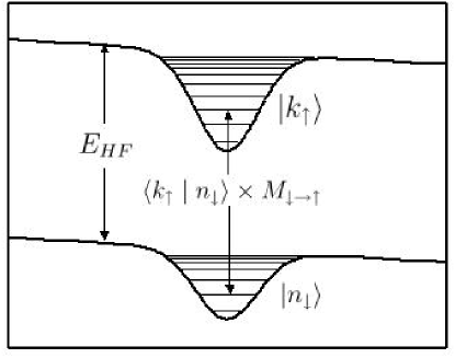
FIG. 1.: The matrix elements for MW-transitions depend on the overlap of the external motion states. The trap shown is a Gaussian trap, and gravity gives the slope.

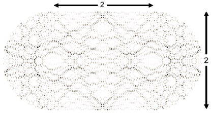
FIG. 2.: Highly excited eigenstate in a Burnimovich billiard (excitation number $\sim 11000$).

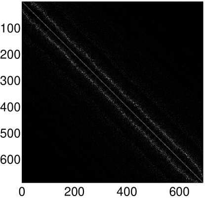
FIG. 3.: $|\left\langle k_{\uparrow}\mid n_{\downarrow}\right\rangle|^{2}$ (the elements of the transform matrix T squared (see text)) for 700 states centered around $n=m\sim 11000$ for the Bunimovich stadium of Fig. 2, perturbed by a shift of 0.004. Distinct sidebands are observed.

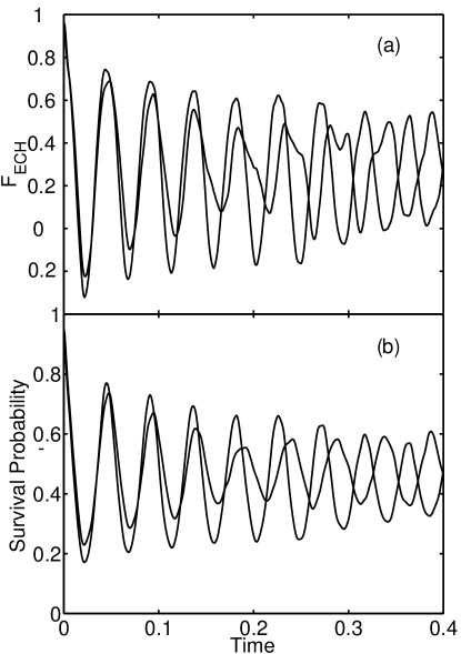
FIG. 4.: a: Echo amplitude from two eigenstates with similar energies in a Burnimovich billiard (excitation number $\sim 11000$), and the perturbation being a shift of 0.008. Clear revivals are seen. b: The same behavior is seen for the survival probability as expected from Eq. 7.

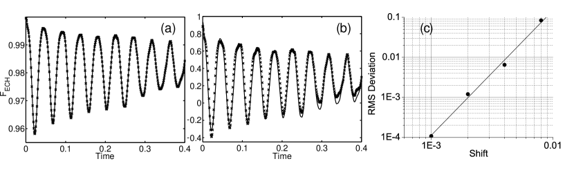
FIG. 5.: a: Solid line: Echo amplitude calculated by full calculation for a shift of 0.001 of a Bunimovich stadium. x: approximation by Eq. 7. Excellent agreement is seen. b: The same as (a) but for a shift of 0.008. Good agreement still exist in spite of very strong oscillations. c: RMS deviation between exact Echo amplitude and perturbative approximation for time 0-0.1 as a function of perturbation (x). It is seen to agree with $\epsilon^{3}$ behavior (solid line).

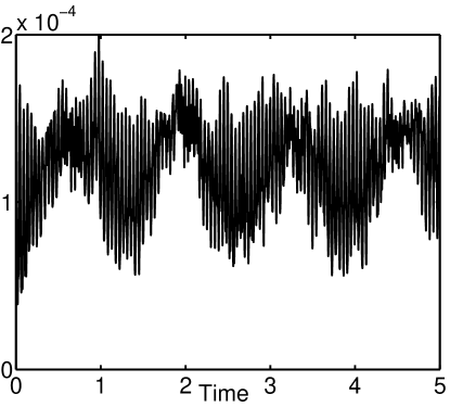
FIG. 6.: The difference between echo amplitude and its perturbative approximation as a function of time for a shift of 0.001 of the Bunimovich Stadium. No divergence is observed even for long times.

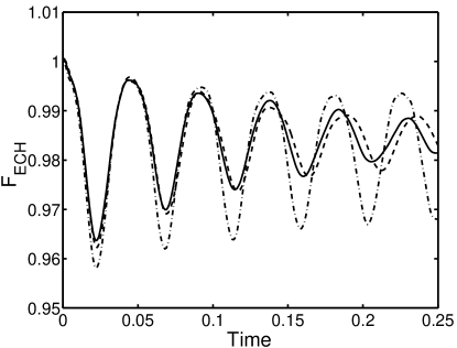
FIG. 7.: Dash-dotted line: Echo amplitude of single eigenstate for a Bunimovich stadium and a shift of 0.001. Dashed line: Semiclassical approximation using Eq. 11 and 12 in Eq. 6. Solid line: Ensemble average of echo amplitudes from 15 adjacent eigenstates. The semiclassical approximation does not resemble the echo from a single eigenstate, but closely resembles the average of just 15 eigenstates. No fitting or scaling is used.

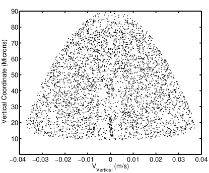
FIG. 8.: Poincaré surface of section for the light-sheet wedge billiard described in the text. The vertical position is plotted as a function of the vertical momentum, when the atom crosses the symmetry axis of the wedge, for a single long trajectory. Phase space is seen to be chaotic.

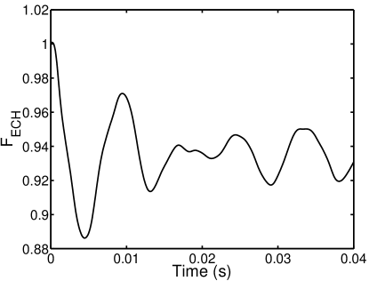
FIG. 9.: Echo coherence for a light sheet wedge billiard described in the text. In spite of the underlying classical dynamics being chaotic oscillations are seen.

REFERENCES

- [1] M. A. Nielsen and I. L. Chuang, Quantum Computation and Quantum Information, Cambridge University Press, 2000.
- [2] E. L. Hahn, Phys. Rev. 80, 580 (1950).
- [3] M. A. Rowe et. al., Quantum Information and Computation. 2, 257 (2002).
- [4] M. F. Andersen, A. Kaplan and N. Davidson, Phys. Rev. Lett. 90, 023001 (2003).
- [5] S. Kuhr et. alt., arXiv:quant-ph/030481.
- [6] V. Milner, J. L. Hanssen, W. C. Campbell and M. G. Raizen, Phys. Rev. Lett. 86, 1514 (2001).
- [7] N. Friedman, A. Kaplan, D. Carasso and N. Davidson, Phys. Rev. Lett. 86, 1518 (2001), A. Kaplan, N. Friedman, M. F. Andersen, Phys. Rev. Lett. 87, 274101 (2001), and M. F. Andersen, A. Kaplan, N. Friedman and N. Davidson, J. Phys. B. 35, 2183 (2002).
- [8] R. A. Jalabert and H. M. Pastawski, Phys. Rev. Lett. 86, 2490 (2001).
- [9] M. F. Andersen, A. Kaplan, T. Grunzweig, and N. Davidson, Communications in Nonlinear Science and Numerical Simulation, 8, 289 (2003).
- [10] D. Cohen, A. Barnett and E. J. Heller, Phys. Rev. E, 63, 046207 (2001), and D. Cohen and T. Kottos, Phys. Rev. E, 63, 036203 (2001).
- [11] It is noted that for some of the data points of [4] the perturbation exceeds strengths where a second order perturbative result it expected to be valid.
- [12] L. A. Bunimovich, Commun. Math. Phys. 65, 295 (1979).
- [13] E. Vergini and M. Saraceno, Phys. Rev. E, 52, 2204 (1995).
- [14] N. Davidson, H. J. Lee, C. S. Adams, M. Kasevich, and S. Chu, Phys. Rev. Lett. 74, 1311 (1995).
- [15] C. Cohen-Tannoudji, J. Dupont-Roc and G. Grynberg, Atom-Photon interactions, John Wiley & Sons Inc. (1992).
- [16] N. F. Ramsey, Molecular Beams, Oxford at the Clarendon Press (1956).
- [17] A. Peres, Phys. Rev. A 30, 1610 (1984)., Joseph Emerson, Yaakov S. Weinstein, Seth Lloyd, and D. G. Cory, Phys. Rev. Lett. 89, 284102 (2002), D. A. Wisniacki, arXiv:nlin.CD/0208044, R. A. Jalabert and H. M. Pastawski, Phys. Rev. Lett. 86, 2490 (2001), T. Prosen and M Znidaric, New J. Phys. 5 109 (2003), R. Sankaranarayanan, and A. Lasshminarayan, Phys. Rev E, In Press, and many more.
- [18] T. Ido, Y. Isoya and, H. Katori, Phys Rev. A 61, 061403 (2000); H. J. Lewandowski, D. M.Harber, D. L. Whitaker, and E. A. Cornell, Phys. Rev. Lett. 88, 070403 (2002); A. Kaplan, M. F. Andersen, and N. Davidson, Phys Rev. A 66, 045401 (2002); H. Haffner, S. Gulde, M. Riebe, G. Lancaster, C. Becher, J. Eschner, F. Schmidt-Kaler, and R. Blatt, Phys. Rev. Lett. 90, 143602 (2003).
- [19] The echo amplitude also characterizes the contrast of Ramsey-like fringes that occur around when the two dark times are not equal.
- [20] A. H. Barnett, Dissipation in Deforming Chaotic Billiards, Ph.D.-thesis (2000).
- [21] A. Barnett, D. Cohen, and E. J. Heller, Phys. Rev. Lett. 85, 1412 (2000), A. Barnett, D. Cohen, and E. J. Heller, J. Phys. A. 34, 413 (2001), and D. Cohen, Ann. Phys. (N.Y.) 283, 175 (2000).
- [22] H. E. Lehtihet and B. N. Miller, Physica (Amsterdam) 21D, 93 (1986).