Efficient extraction of quantum Hamiltonians from optimal laboratory data

Abstract

Optimal Identification (OI) is a recently developed procedure for extracting optimal information about quantum Hamiltonians from experimental data using shaped control fields to drive the system in such a manner that dynamical measurements provide maximal information about its Hamiltonian. However, while optimal, OI is computationally expensive as initially presented. Here, we describe the unification of OI with highly efficient global, nonlinear map-facilitated data inversion procedures. This combination is expected to make OI techniques more suitable for laboratory implementation. A simulation of map-facilitated OI is performed demonstrating that the input-output maps can greatly accelerate the inversion process.

I Introduction

A general goal in atomic and molecular physics is to quantitatively predict quantum dynamics from knowledge of the system Hamiltonian. However, sufficiently accurate information about these Hamiltonians is still lacking for many applications. Although the capabilities of ab initio methods are improving, they remain unable to provide the quantitative accuracy needed to predict many quantum dynamical phenomena and data inversion remains the most reliable source of precision information about quantum Hamiltonians. But, traditional data inversion techniques are hindered by the fact that (a) spectroscopic and collision data only provide information about limited portions of the the desired interactions and (b) the relationships between quantum Hamiltonians and their corresponding observables are generally nonlinear Geremia et al. (2001a).

The recently proposed optimal identification (OI) Geremia and Rabitz (2002); Geremia and Rabitz (2003a) procedure provides a new approach to quantum system Hamiltonian identification through laboratory data inversion. The operating principle behind OI is to improve the information content of the data by driving the quantum system using a tailored control field (e.g., a shaped laser pulse). If suitably chosen, the control field forces the data to become highly sensitive to otherwise inaccessible portions of the Hamiltonian and therefore enables a high fidelity inversion. A key component of the OI concept exploits the fact that the inversion will generally produce a family, or distribution, of Hamiltonians that are consistent with the laboratory data Geremia and Rabitz (2001a, 2003b). The breadth of this inversion family provides a figure of merit for the quality of the inversion. The limiting experimental factors that prevent the inverted family of Hamiltonians from collapsing down to a single (i.e., completely certain) member arise from two sources. First, the finite precision of the data reduces the resolving power of the measurements and makes it possible for multiple Hamiltonians to be consistent with the data to within its experimental error. Second, Hamiltonians that differ in ways for which the data is insensitive also reduces the inversion quality. OI operates by attempting to drive the quantum system into a dynamical state where the associated experimental errors are least compromising, yet where the measurements provide distinguishing power between Hamiltonians to narrow down the family consistent with the data.

As originally formulated, the OI algorithm requires performing a large number of global, nonlinear data inversions, each of which can be computationally expensive Geremia and Rabitz (2003a). Resolving the members of the inversion family consistent with the data might require extracting hundreds of distinct Hamiltonians involving numerous solutions of the Schrödinger equation. In this paper, we demonstrate that it is possible to greatly reduce the computational challenge of performing OI by incorporating map-facilitated inversion techniquesGeremia and Rabitz (2001a, 2003b); Geremia and Rabitz (2001b) that have been specifically developed for efficiently finding these solution families. A map is a predetermined quantitative input$\to$output relationship which can alleviate the expense of repeatedly solving the Schrödinger equation Geremia et al. (2001a).

This paper provides a detailed description of the algorithm demonstrated in Ref. Geremia and Rabitz (2002) for extracting both internal Hamiltonian and transition dipole moment matrix elements from simulated laser pulse shaping and population data. Section II reviews the OI concept introduced in Ref. Geremia and Rabitz (2003a) and then extends this procedure to incorporate map-facilitated inversion. Section III provides a detailed description and in-depth analysis of the simulations that were presented in Ref. Geremia and Rabitz (2002).

II Algorithm

The principal behind the OI algorithm is to optimize an external control field that drives the system in a manner similar to the learning-loop techniques utilized in many current coherent quantum control experiments. The distinction between OI and the latter control experiments lies in the optimization target: OI is guided to optimize the extracted Hamiltonian information. The OI learning algorithm programs a control pulse-shaper to drive the quantum system followed by the collection of associated dynamical observations. In practice, the control optimization is performed over a discrete set of variables (control “knobs”), $\mathbf{c}\equiv\{c_{1},\ldots,c_{N_{c}}\}$,

$$E(t)\to E(t;c_{1},c_{2},\ldots,c_{N_{c}})$$ (1)

where the space of accessible fields is defined by varying each $c_{i}$ over a range , $c_{i}^{(min)}\leq c_{i}\leq c_{i}^{(max)}$. For each trial field, $E_{k}(t;\mathbf{c}_{k})$, $k=1,2,\ldots$, a set of measurements, $\Phi^{(lab)}_{k}$, are performed on the system. Each trial field yields $M$ individual measurements (e.g., the populations of $M$ different quantum states), $\Phi^{(lab)}_{k}=\{\Phi^{(lab)}_{k,1},\ldots,\Phi^{(lab)}_{k,M}\}$, with associated errors, $\{\varepsilon^{(lab)}_{k,1},\ldots,\varepsilon^{(lab)}_{k,M}\}$.

Inversion is performed by adopting a discrete set of variables, $\mathbf{h}=\{h_{1},\ldots,h_{N_{h}}\}$ used to distinguish one trial Hamiltonian from another. There are many possible ways to define these Hamiltonian variables, and the best representation must be selected to suit the quantum system being inverted, but in general, a sufficiently flexible and accurate description of Hamiltonian space requires a large number of variables, $N_{h}\gg 1$. Inversion is accomplished by minimizing,

$$\mathcal{J}_{\mathrm{inv}}(\mathbf{h};\Phi^{(lab)}_{k})=\frac{1}{M}\sum\limits_{m=1}^{M}\left\{\begin{array}[]{c@{\quad:\quad}l}0&|\Phi^{(lab)}_{k,m}-\Phi_{k,m}[\mathbf{h}]|\leq\varepsilon^{(lab)}_{k,m}\\ \left\|\frac{\Phi^{(lab)}_{k,m}-\Phi_{k,m}[\mathbf{h}]}{\Phi^{(lab)}_{k,m}}\right\|^{2}&|\Phi^{(lab)}_{k,m}-\Phi_{k,m}[\mathbf{h}]|>\varepsilon^{(lab)}_{k,m}\end{array}\right.+\hat{K}\mathbf{h}$$ (2)

where $\Phi_{k,m}[\mathbf{h}]$ is the $m^{th}$ ($m=1,\ldots,M$) observable’s computed value for the trial Hamiltonian, $\mathbf{h}$, under the influence of the external field, $E_{k}(t)$. Optionally, a regularization operator, $\hat{K}$, acting on the Hamiltonian, $\mathbf{h}$, can be used to incorporate a priori behavior, such as smoothness, proper asymptotic behavior, symmetry, etc., into the inverted Hamiltonian Miller (1970); Ho and Rabitz (1989); Geremia and Rabitz (2001a). While the data error distributions are assumed to have hard bounds, $\varepsilon^{(lab)}_{k,m}$, in Eq. (2), other distributions could be used as well.

The output of the inversion optimization is a set of $N_{s}$ Hamiltonians, $\{\mathbf{h}^{*}_{1},\ldots,\mathbf{h}^{*}_{N_{s}}\}$, that each ideally reproduce the measured observable, $\Phi^{(lab)}_{k}$, to within its experimental error. The upper and lower bounds of each inverted variable defines the family,

$${}^{<}\!h_{i}^{*} = \min\limits_{s}\{h_{s,i}^{*}\}$$ (3)

$${}^{>}\!\!h_{i}^{*} = \max\limits_{s}\{h_{s,i}^{*}\}$$ (4)

where $h_{s,i}^{*}$ is the $i^{th}$ Hamiltonian variable from the $s^{th}$ member of $\mathbf{H}^{*}$. The uncertainty in each Hamiltonian variable, $\Delta h_{i}^{*}$, is quantified by the width of its corresponding solution space,

$$\Delta h_{i}^{*}=^{>}\!\!h_{i}^{*}-^{<}\!h_{i}^{*}$$ (5)

and the width of the family for each Hamiltonian variable is used to compute the uncertainty in the full inversion, $\Delta\mathbf{H}^{*}[\,E_{k}(t)\,]$,

$$\Delta\mathbf{H}^{*}[\,E_{k}(t)\,] = \frac{1}{N_{s}}\sum_{s=1}^{N_{s}}\mathcal{J}_{\mathrm{inv}}[\mathbf{h}^{*}_{s};\Phi^{(lab)}_{k}]+$$

$$\alpha\frac{1}{N_{h}}\sum_{i=1}^{N_{h}}\left|\,\frac{2\Delta h_{i}^{*}}{{}^{<}\!h_{i}^{*}+^{>}\!\!h_{i}^{*}}\,\right|$$

where $\mathbf{h}^{*}_{s}$ is the $s^{th}$ member of the inversion family found from $E_{k}(t)$ and $\mathcal{J}_{\textrm{inv}}$ is given by Eq. (2). The first term in Eq. (II) measures the ability of the inversion family to reproduce the data and the second measures the inversion uncertainty with $\alpha>0$ being a coefficient that balances them.

This measure of inversion uncertainty is used to guide the control optimization where the objective is to optimize $\Delta\mathbf{H}^{*}$ over the space of accessible fields by minimizing the control cost function,

$$\mathcal{J}_{c}[\,E(t;\mathbf{c})\,] = \Delta\mathbf{H}^{*}[\,E(t;\mathbf{c})\,]+$$

$$\beta\sum_{i=1}^{N_{c}}\left|\frac{c_{i}-c_{i}^{(min)}}{c_{i}^{(max)}-c_{i}^{(min)}}\right|$$

where the first term reduces inversion error and the second removes extraneous field components relative to their minimum value, balanced by $\beta>0$.

The result of the control field optimization is a set of laboratory data and its corresponding inversion results, $\{E_{k}^{*}(t),\Phi^{*}_{k},\varepsilon^{*}_{k},\mathbf{h}^{*}_{k}\}$ that provides the best possible knowledge of the unknown Hamiltonian provided by the set of accessible optimal control fields. This inversion result provides the Optimal Identification of the quantum system with uncertainty,

$$\Delta h_{i}\!\!\stackrel{{\scriptstyle\raisebox{-8.0pt}[-3.01389pt][0.0pt]{*}}}{{\raisebox{-1.0pt}{*}}}=\,^{>}\!h_{i}\!\!\!\stackrel{{\scriptstyle\raisebox{-8.0pt}[-3.01389pt][0.0pt]{*}}}{{\raisebox{-1.0pt}{*}}}-^{<}\!h_{i}\!\!\!\stackrel{{\scriptstyle\raisebox{-8.0pt}[-3.01389pt][0.0pt]{*}}}{{\raisebox{-1.0pt}{*}}}$$ (8)

where ${}^{>}\!h_{i}\!\!\!\stackrel{{\scriptstyle\raisebox{-8.0pt}[-3.01389pt][0.0pt]{*}}}{{\raisebox{-1.0pt}{*}}}$ and ${}^{<}\!h_{i}\!\!\!\stackrel{{\scriptstyle\raisebox{-8.0pt}[-3.01389pt][0.0pt]{*}}}{{\raisebox{-1.0pt}{*}}}$ are computed using Eqs. (3) and (4) for the optimal data.

The most expensive operation in OI is the many solutions of Schrödinger’s equation required in the inversion component of the algorithm. The map-facilitated inversion aims to alleviate this costly operation. Computing quantum observables, $\Phi_{k}[\mathbf{h}]$, from a given Hamiltonian, $\mathbf{h}$, and control field, $E_{k}(t;\mathbf{c}_{k})$, defines a forward map,

$$f\,:\,(\mathbf{h};E_{k})\rightarrow\Phi_{k}[\mathbf{h}]$$ (9)

that is parameterized by the control field, $E_{k}(t)$. In the initial presentation of OI, this map is explicitly evaluated each time a trial Hamiltonian is tested to determine if it is consistent with the laboratory data. However, it has recently been found that it is possible to pre-compute this map to high accuracy by sampling $f(\mathbf{h};E_{k})$ for a representative collection of Hamiltonians.

Although it is generally impossible to resolve $f$ on a full grid in $\mathbf{h}$-space due to exponential sampling complexity in $N_{h}\gg 1$ dimensions, it has been found Geremia et al. (2001a) that an accurate nonlinear map can often be constructed using the functional form,

$$f(\mathbf{h};E_{k}) = f_{0}(E_{k})+\sum_{i=1}^{N_{h}}f_{i}(h_{i};E_{k})+\sum_{i<j}^{N_{h}}f_{ij}(h_{i},h_{j};E_{k})$$ (10)

$$+\cdots+f_{1\cdots N_{h}}(h_{1},\ldots,h_{N_{h}};E_{k})$$

where $f_{0}(E_{k})$ is a constant term, the functions, $f_{i}(h_{i};E_{k})$, dependent upon a single variable, $h_{i}$, the functions $f_{ij}(h_{i},h_{j};E_{k})$ depend upon two variables, $h_{i}$ and $h_{j}$, etc. Expansions of the form in Eq. (10) belong to a family of multivariate representations used to capture the input$\to$output relationships of many high-dimensional physical systemsAlis and Rabitz (1999); Rabitz et al. (1999); Shorter and Rabitz (2000); Shorter et al. (1999); Rabitz and Shim (1998); Shim and Rabitz (1998); Rabitz and Shim (1999); Geremia et al. (2001a, b). It has been shown that Eq. (10) converges to low order, $L\ll N_{h}$ for many Hamiltonian$\to$observable maps. A low order, converged map expansion can be truncated after its last significant order without sacrificing accuracy or nonlinearity which dramatically reduces the computational labor of constructing the map. The specifics for how the individual expansion functions should be evaluated can be found in previous papersGeremia et al. (2001a); Geremia and Rabitz (2001b); Geremia et al. (2001b).

Map-facilitated OI operates by replacing the step of explicitly computing $\Phi_{k}[\mathbf{h}]$ in Eq. (2) with the value $f(\mathbf{h};E_{k})$ obtained by evaluating the functional map in Eq. (10) which serves as a high-speed replacement for solving the Schrödinger equation. The map (or potentially multiple maps if this is necessary to ensure sufficient accuracy Geremia and Rabitz (2001a)) must be constructed as a preliminary step prior to initiating the inversion optimization. Since map construction requires knowledge of the control field, it may not be possible to pre-compute all of the maps prior to executing the full OI loop. Instead, a new map will generally need to be constructed for each trial laser pulse.

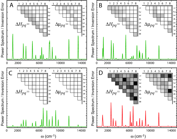
Figure 1: (color online) Comparison of optimal versus conventional Hamiltonian identification. In plots (A-C) the identification error (darker shading implies larger inversion error) respectively reflects OI’s performed using 1, 2, and 4 samples of the populations during the wavepacket evolution. Increasing the number of data points available to the OI process improves the quality of the extracted Hamiltonian. Plot (D) represents a conventional identification where the populations were sampled 25 times during the time evolution. Despite using significantly less data, OI obtained higher quality Hamiltonian information.

III Illustration

The map-facilitated OI algorithm was simulated for an 8–level Hamiltonian8St chosen to resemble vibrational transitions in a molecular system where the objective was to extract optimal information about the molecular Hamiltonian, $H$, and dipole moment, $\mu$, for a system having the total Hamiltonian,

$$\hat{H}=H-\mu\cdot E_{k}(t)\,.$$ (11)

The control fields have the form,

$$E_{k}^{(j)}(t)=\exp\left(\frac{-(t-T/2)^{2}}{2s^{2}}\right)\sum_{l}A_{l}^{(j)}\cos(\omega_{l}t+\theta_{l}^{(j)})$$ (12)

where the $\omega_{l}$ are the resonance frequencies8St of $H$, $A_{l}^{(j)}$, their corresponding amplitudes and $\theta_{l}^{(j)}$, their associated phases. Control field noise was modeled as parametric uncertainties in the $A_{l}$ and $\theta_{l}$,

$$A_{l}^{(j)}=(1+\gamma_{A_{l}}^{(j)})A_{l},\hskip 14.22636pt\theta_{l}^{(j)}=(1+\gamma_{\theta_{l}}^{(j)})\theta_{l}$$ (13)

where different random values between $\pm\varepsilon^{(fld)}$ were chosen for $\gamma_{A_{l}}^{(j)}$ and $\gamma_{\theta_{l}}^{(j)}$ for each pulse.

The OI simulation involved learning the matrix elements of the Hamiltonian, $H_{pq}=\langle p|H|q\rangle$, and dipole moment, $\mu_{pq}=\langle p|\mu|q\rangle$ for a chosen basis, $|p\rangle$, $p=1,\ldots,8$ . Simulated laboratory data was generated by propagating the initial wavefunction under the influence of the applied control field from its initial state and computing the populations (in the chosen basis, $|p\rangle$) at various times, $t_{q}$, during the evolution. Each population “measurement” was averaged over $D=100$ replicate observations for a collection of noise-contaminated fields, $\{E_{k}^{(j)}(t)\}$, $j=1,\ldots,D$, centered around the nominal field, $E_{k}(t)$ to simulate experimental uncertainty in the laser pulse-shaping process. Measurement error, $\varepsilon^{(lab)}$, was introduced into the population observations according to,

$$\Phi^{(lab)}_{k,m}=\Big{\langle}(1+\rho_{ij})\,p_{i}\big{(}t_{q};[E_{k}^{(j)}(t)]\big{)}\Big{\rangle}_{j=1,\ldots,D}$$ (14)

where the $\rho_{ij}$ were chosen randomly between $\pm\varepsilon^{(obs)}$, the relative error in each population observation. A different random value, $\rho_{ij}$, was selected for every simulated measurement.

Equation (II) was minimized over $\mathbf{c}=\{A_{l},\theta_{l}\}$ using a steady state GA with a population size of 30, a mutation rate of 5$\%$, and a cross-over rate of 75$\%$. The pulse parameters where chosen to be $T=1.0$ ps and $s=200$ fs, the amplitudes, $A_{l}$, were allowed to vary over [0,1] V/Å, and the phases were allowed to vary over [0,2$\pi$] rad. The laboratory measurement error was assumed to be $\varepsilon^{(lab)}_{k}=2\%$, the field error, $\varepsilon^{(fld)}=1\%$ and the observation times, $t_{q}$, were uniformly spaced over the evolution period (i.e., the time between observations was $\Delta t=T/Q$ with $Q$ = 1, 2 or 4). At each time, the full set of 8 populations was measured. The parameters, $\alpha$ in Eq. (II) and $\beta$ in Eq. (II), were ramped from 1$\times$10^-4 to 1$\times$10^-2 over the GA evolution, although the optimization was insensitive to the exact choices of $\alpha$ and $\beta$. Typically $\sim$50 generations, or approximately 800 trial fields, were needed for GA convergence.

Global inversion to identify the Hamiltonian family corresponding to the data, $\Phi^{(lab)}_{k}$, was performed by minimizing Eq. (2) using a map-facilitated inversion algorithm. For each inversion, the family of consistent Hamiltonians was identified using a steady-state GA with a cross-over rate of 70$\%$ and a mutation rate of 5$\%$. The trial family size was $N_{s}=500$ and the GA population size was $N_{p}=100$. The Hamiltonian-space map variables, $h_{i}$, were the matrix elements of the molecular Hamiltonian, $H_{mn}$, and the the dipole, $\mu_{mn}$. For the eight-level system, there were 36 Hamiltonian elements (symmetric, upper-triangle including the diagonal) and 28 transition dipole moments (symmetric, upper-triangle without the diagonal) producing an $N_{h}=64$-dimensional map. All maps were constructed to first order, $L=1$, and $S=6$ sample points were used to resolve each map function for interpolation. The Hamiltonian-space domain extended $\pm 30\%$ around its nominal value (each matrix element was assumed known to $\pm 15\%$ prior to the present identification). Typical map construction required an average of 84 seconds to perform on an SGI MIPS single processor machine, and map-facilitated inversion required an average of 51 seconds to converge. A single evaluation of the Hamiltonian$\to$population map typically required $\sim 1$ ms, while a similar solution of the Schröinger equation for this system took $\sim 2$ s. This difference is the origin of the savings associated with map-facilitated OI.

The performance of the map-facilitated OI algorithm was assessed with the following four tests:

1. An OI was performed using populations measured at $Q=1$ time, $t_{1}=T$, producing 8 observations for the 64 unknowns.

2. An OI was performed using populations measured at $Q=2$ times, $t_{1}=T/2$ and $t_{2}=T$, producing 16 observation for the 64 unknowns.

3. An OI was performed using populations measured at $Q=4$ times, $t_{q}=qT/4$, $q=1,\ldots,4$, producing 32 observations for the 64 unknowns.

4. A conventional inversion (with a randomly selected field) was performed using populations sampled at $Q=25$ times, $t_{q}=qT/25$, $q=1,\ldots,25$, producing 200 observations for the 64 unknowns.

The power spectra of the optimal control fields for the $Q=$ 1, 2, and 4 OI inversions are shown in Figure 1 along with a graphical depiction of the OI error, $\Delta h_{i}\!\!\stackrel{{\scriptstyle\raisebox{-8.0pt}[-3.01389pt][0.0pt]{*}}}{{\raisebox{-1.0pt}{*}}}$. For a single time sample, $Q=1$, the overall inversion error, computed as the average, $2\langle\Delta h_{i}\!\!\stackrel{{\scriptstyle\raisebox{-8.0pt}[-3.01389pt][0.0pt]{*}}}{{\raisebox{-1.0pt}{*}}}/(^{<}\!h_{i}\!\!\!\stackrel{{\scriptstyle\raisebox{-8.0pt}[-3.01389pt][0.0pt]{*}}}{{\raisebox{-1.0pt}{*}}}+^{>}\!h_{i}\!\!\!\stackrel{{\scriptstyle\raisebox{-8.0pt}[-3.01389pt][0.0pt]{*}}}{{\raisebox{-1.0pt}{*}}})\rangle$, was found to be $3.67\%$. Figure 1(A) shows that the majority of the error was contained in and around the diagonal elements of $H$ (note that the Hamiltonian is not diagonal in the chosen basis, $|p\rangle$). The average relative error in the dipole, $0.9413\%$, was significantly smaller, and the majority of dipole uncertainty appeared in the $v$$\to$$v+2$ elements. The inversion error for the two-point, $Q=2$, OI demonstration was reduced to $2.910\%$ for the molecular Hamiltonian. Again, the majority of the inversion uncertainty resides in the diagonal elements of $H$. The transition dipole moment elements also improved with an overall average uncertainty of $0.6270\%$.

The inversion error, $\Delta h_{i}\!\!\stackrel{{\scriptstyle\raisebox{-8.0pt}[-3.01389pt][0.0pt]{*}}}{{\raisebox{-1.0pt}{*}}}$, for a simulated OI utilizing data at $Q=4$ times, is essentially eliminated. The average uncertainty in both the molecular Hamiltonian elements and in the transition dipoles is an order of magnitude smaller than the simulated error in the data, $\varepsilon^{(lab)}_{k}$ = 2 %. The most dramatic demonstration of the OI’s capabilities is seen by comparing Figure 1(C and D). The plot in (D) represents a conventional inversion, performed using a randomly selected field and $Q=25$ time samples, compared to $Q=4$ for OI. The conventional inversion therefore had access to $M=200$ data points while the map-facilitate OI demonstration only had $M$ = 32. Despite what would appear to be a significant advantage in the amount of available data, the conventional inversion displays greater than two orders of magnitude more error. The conventional dipole moment inversion produced an average uncertainty of $19.5\%$ and the precision in the molecular Hamiltonian was $28.1\%$. The map-facilitated OI found a control field and associated data that essentially prevented the laboratory noise from propagating into the identified Hamiltonian information.

IV Conclusion

We have presented simulated experimental data that demonstrates the utility of map-facilitate Optimal Identification for the real-time laboratory identification of quantum Hamiltonians from dynamical physical observable data. The central concept behind OI is that by suitably driving the quantum system in an optimal manner, it is possible to extract high-precision information about all relevant aspects of its Hamiltonian despite finite laboratory error in both the external control fields and measured data. In this demonstration of map-facilitated OI, it was possible to improve the computational efficiency of data inversion by more than an order of magnitude compared to the initial presentation of the OI concept Geremia and Rabitz (2002). This increased efficiency is ultimately expected to aid, if not be essential, for the practical implementation of OI.