Gaussian Decoherence from Spin Environments

Abstract

We examine an exactly solvable model of decoherence – a spin-system interacting with a collection of environment spins. We show that in this model (introduced some time ago to illustrate environment–induced superselection) generic assumptions about the coupling strengths lead to a universal (Gaussian) suppression of coherence between pointer states. We explore the regimes of validity of these results and discuss their relation to the spectral features of the environment and to the Loschmidt echo (or fidelity). Finally, we comment on the observation of such time dependence in spin echo experiments.

A single spin–system ${\cal S}$ (with states $\left\{\left|0\right>,\left|1\right>\right\}$) interacting with an environment ${\cal E}$ of many independent spins ($\left\{\left|\uparrow_{k}\right>,\left|\downarrow_{k}\right>\right\}$, $k=1..N$) through the Hamiltonian

$${\cal H_{SE}}=\left(\left|0\right>\left<0\right|-\left|1\right>\left<1\right|\right)\sum_{k=1}^{N}\frac{g_{k}}{2}\left(\left|\uparrow_{k}\right>\left<\uparrow_{k}\right|-\left|\downarrow_{k}\right>\left<\downarrow_{k}\right|\right)$$ (1)

may be the simplest solvable model of decoherence in spin systems. It was introduced some time ago Zurek82 to show that relatively straightforward assumptions about the dynamics can lead to the emergence of a preferred set of pointer states due to environment–induced superselection (einselection) Zurek82 ; deco . Such models have gained additional importance in the past decade because of their relevance to quantum information processing QIP .

The purpose of our paper is to show that – with a few additional natural and simple assumptions – one can evaluate the exact time dependence of the reduced density matrix, and demonstrate that the off–diagonal components display a Gaussian (rather than exponential) decay. In effect, we exhibit a simple soluble example of a situation where the usual Markovian Kossakowski assumptions about the evolution of a quantum open system are not satisfied at all times. Apart from their implications for decoherence, our results are also relevant to quantum error correction ErrorCorrection where precise precise knowledge of the dynamics is essential to select an efficient strategy.

To demonstrate the Gaussian time dependence of decoherence we first write down a general solution for the model given by Eq. (1). Starting with:

$$\left|\Psi_{\cal SE}(0)\right>=(a\left|0\right>+b\left|1\right>)\bigotimes_{k=1}^{N}\left(\alpha_{k}\left|\uparrow_{k}\right>+\beta_{k}\left|\downarrow_{k}\right>\right),$$ (2)

the state of ${\cal SE}$ at an arbitrary time is given by:

$$\left|\Psi_{\cal SE}(t)\right>=a\left|0\right>\left|{\cal E}_{0}(t)\right>+b\left|1\right>\left|{\cal E}_{1}(t)\right>$$ (3)

where

$$\left|{\cal E}_{0}(t)\right> = \bigotimes_{k=1}^{N}\left(\alpha_{k}e^{ig_{k}t/2}\left|\uparrow_{k}\right>+\beta_{k}e^{-ig_{k}t/2}\left|\downarrow_{k}\right>\right)$$ (4)

$$= \left|{\cal E}_{1}(-t)\right>.$$

The reduced density matrix of the system is then:

$$\rho_{\cal S} = {\rm Tr}_{\cal E}\left|\Psi_{\cal SE}(t)\right>\left<\Psi_{\cal SE}(t)\right|$$ (5)

$$= |a|^{2}\left|0\right>\left<0\right|+ab^{*}r(t)\left|0\right>\left<1\right|$$

$$+ a^{*}br^{*}(t)\left|1\right>\left<0\right|+|b|^{2}\left|1\right>\left<1\right|,$$

where the decoherence factor $r(t)=\left<{\cal E}_{1}(t)|{\cal E}_{0}(t)\right>$ can be readily obtained:

$$r(t) = \prod_{k=1}^{N}\left(|\alpha_{k}|^{2}e^{ig_{k}t}+|\beta_{k}|^{2}e^{-ig_{k}t}\right).$$ (6)

It is straightforward to see that $r(0)=1$ and for $t>0$ it decays rapidly to zero, so that the typical fluctuations of the off-diagonal terms of $\rho_{\cal S}$ will be small for large environments, since:

$$\left<|r(t)|^{2}\right>=2^{-N}\prod_{k=1}^{N}\left(1+(|\alpha_{k}|^{2}-|\beta_{k}|^{2})^{2}\right),$$ (7)

Here $\left<...\right>$ denotes a long time average Zurek82 . Clearly, $\left<|r(t)|^{2}\right>\underset{N\rightarrow\infty}{\longrightarrow}0$, leaving $\rho_{\cal S}$ approximately diagonal in a mixture of the pointer states $\left\{\left|0\right>,\left|1\right>\right\}$ which retain preexisting classical correlations.

This much was known since Zurek82 . The aim of this paper is to show that, for a fairly generic set of assumptions, the form of $r(t)$ can be further evaluated and that – quite universally – it turns out to be approximately Gaussian in time. Thus, the simple model of Ref. Zurek82, predicts a universal (Gaussian) form of the loss of quantum coherence, whenever the couplings $g_{k}$ of Eq. 1 are sufficiently concentrated near their average value so that their standard deviation $\left<(g_{k}-\left<g_{k}\right>)^{2}\right>$ exists and is finite. When this condition is not fulfilled other sorts of time dependence become possible. In particular, $r(t)$ may be exponential when the distribution of couplings is a Lorentzian.

To obtain our main result we carry out the multiplication of Eq.(6), re–expressing $r(t)$ as a sum:

$$r(t) = \prod_{k=1}^{N}|\alpha_{k}|^{2}e^{it\sum_{n}g_{n}}+\sum_{l=1}^{N}|\beta_{l}|^{2}\prod_{k\neq l}^{N}|\alpha_{k}|^{2}\times$$ (8)

$$e^{it(-g_{l}+\sum_{n\neq l}g_{n})}+\sum_{l=1}^{N}\sum_{m\neq l}^{N}|\beta_{l}|^{2}|\beta_{m}|^{2}\times$$

$$\prod_{k\neq l,m}^{N}|\alpha_{k}|^{2}e^{\left[it(-g_{l}-g_{m}+\sum_{n\neq l,m}^{N}g_{n})\right]}+...$$

There are $\binom{N}{0}$, $\binom{N}{1}$, $\binom{N}{2}$, … etc. terms in the consecutive sums above. The binomial pattern is clear, and can be made even more apparent by assuming that $\alpha_{k}=\alpha$ and $g_{k}=g$ for all $k$. Then,

$$r(t)=\sum_{l=0}^{N}\binom{N}{l}|\alpha|^{2(N-l)}|\beta|^{2l}e^{ig(N-2l)t},$$ (9)

i.e., $r(t)$ is the binomial expansion of $r(t)=\left(|\alpha|^{2}e^{igt}+|\beta|^{2}e^{-igt}\right)^{N}$.

We now note that, as follows from the Laplace-de Moivre theorem Gnedenko , for sufficiently large $N$ the coefficients of the binomial expansion of Eq. (9) can be approximated by a Gaussian:

$$\binom{N}{l}|\alpha|^{2(N-l)}|\beta|^{2l}\simeq\frac{\exp{\left[-\frac{(l-N|\beta|^{2})^{2}}{2N|\alpha\beta|^{2}}\right]}}{\sqrt{2\pi N|\alpha\beta|^{2}}}.$$ (10)

This limiting form of the distribution of the eigenenergies of the composite ${\cal SE}$ system immediately yields our main result: $r(t)$ is approximately Gaussian since it is a Fourier transform of an approximately Gaussian distribution of the energies resulting from all the possible combinations of the couplings with the environment.

The set of all the resulting energies must have an (approximately) Gaussian distribution. This behavior is generic, a result of the law of large numbers Gnedenko : these energies can be thought of as being the terminal points of an $N$–step random walk. The contribution of the $k$–th spin of the environment to the random energy is $+g$ or $-g$ with probability $|\alpha|^{2}$ or $|\beta|^{2}$ respectively (Fig. 1 a).

The same argument can be carried out in the more general case of Eq. (8). The “random walk” picture that yielded the distribution of the couplings remains valid (see Fig. 1 b). However, now the individual steps in the random walk are not all equal. Rather, they are given by the set $\left\{g_{k}\right\}$ (see Eq. 1) with each step $g_{k}$ taken just once in a given walk. There are $2^{N}$ such distinct random walks, each contributing with the weight given by the product of the relevant $|\alpha_{k}|^{2}$ and $|\beta_{k}|^{2}$ to the sum of Eq. (8). This exponential proliferation of the contributing coupling energies allows one to anticipate rapid convergence to the universal Gaussian form of the decoherence factor $r(t)$.

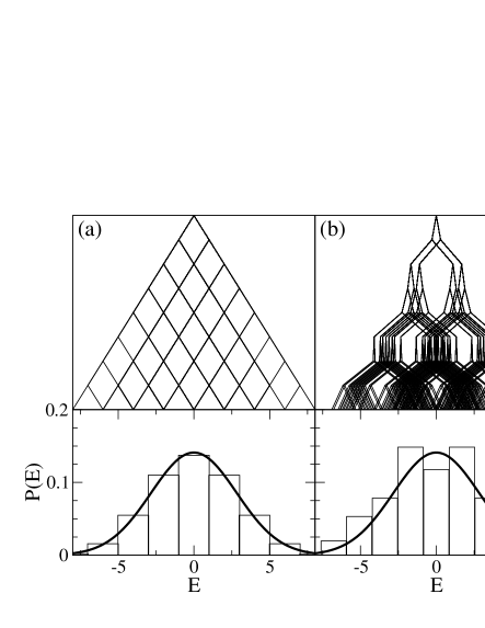
Figure 1: The distribution of the energies obtains from the random walks with the steps given by the coupling size and in the direction ($+g_{k}$ or $-g_{k}$) biased by the probabilities $|\alpha_{k}|^{2}$ and $|\beta_{k}|^{2}$ as in Eq. (15) (although in these examples we set $|\alpha_{k}|^{2}=1/2$). (a) When all the couplings have the same size $g_{k}=g$ (Eq. (9)), a simple Newton’s triangle leads to an approximate Gaussian for the distribution of energies. (b) When the couplings differ from step to step (Eq. (8)), the resulting distribution still has a approximately Gaussian envelope for large $N$.

Indeed, we can regard the energies resulting from the sums of $g_{k}$’s as a random variable. Its probability distribution is given by products of the corresponding weights. That is, the typical term in Eq. 8 is of the form:

$$p_{W}e^{iE_{W}t}\equiv\left(\prod_{k\in W^{+}}|\alpha_{k}|^{2}e^{ig_{k}t}\right)\left(\prod_{k\in W^{-}}|\beta_{k}|^{2}e^{-ig_{k}t}\right).$$ (11)

The resulting terminal energy is

$$E_{W}=\sum_{k\in W^{+}}g_{k}-\sum_{k\in W^{-}}g_{k},$$ (12)

and the cumulative weight $p_{W}$ is given by the corresponding product of $|\alpha_{k}|^{2}$ and $|\beta_{k}|^{2}$. Each such specific random walk $W$ corresponding to a given combination of right ($k\in W^{+}$) and left ($k\in W^{-}$) “steps” (see Fig. 1) contributes to the distribution of energies only once. The terminal points $E_{W}$ may or may not be degenerate: As seen in Fig. 1, in the degenerate case, the whole collection of $2^{N}$ random walks “collapses” into $N+1$ terminal energies. More typically, in the degenerate case (also displayed in Fig. 1), there are $2^{N}$ different terminal energies $E_{W}$. In both cases, the “envelope” of the distribution $P(E_{W})$ should be Gaussian, as we shall argue below.

We note that the decoherence factor $r(t)$ can be viewed as the characteristic function Gnedenko (i.e., the Fourier transform) of the distribution of eigenenergies $E_{W}$. Thus,

$$r(t)=\int e^{iEt}\eta(E)dE,$$ (13)

where the strength function $\eta(E)$, also known as the local density of states (LDOS) LDOS is defined in general as

$$\eta(E)=\sum_{\lambda}|\left<\Psi_{\cal SE}(0)|\phi_{\lambda}\right>|^{2}\delta(E-E_{\lambda}).$$ (14)

Above $\left|\phi_{\lambda}\right>$ are the eigenstates of the full Hamiltonian and $E_{\lambda}$ its eigenenergies. In our particular model (Eq. 1) the eigenstates are associated with all possible random walks in the set $W$, and therefore

$$\eta(E)=\sum_{W}p_{W}\delta(E-E_{W}).$$ (15)

The discussion of decoherence in our model is thus directly related to the study of the characteristic function of the distribution of coupling energies $\eta(E)$. Moreover, since the $E_{W}$’s are sums of $g_{k}$’s (that we assume independent of each other), $r(t)$ is itself a product of characteristic functions of the distributions of the couplings $\{g_{k}\}$, as we have already seen in the example of Eq. (6). Thus, the distribution of $E_{W}$ belongs to the class of the so–called infinitely divisible distributions Gnedenko ; breiman .

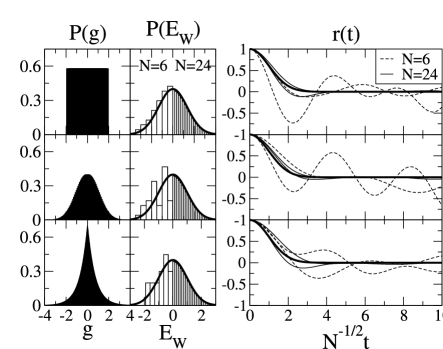
Figure 2: (Left panels) Assumed distribution of the couplings $g_{k}$. (Center panels) Resulting distribution of the eigenenergies $E_{W}$ (center panels) for $N=6$ ($E_{W}<0$) and $N=24$ ($E_{W}>0$). In the case of $|\alpha_{k}|^{2}=1/2$ this distribution is in effect the “strength function” (local density of states). (Right panels) Decoherence factor $r(t)$ for different initial conditions with $N=6$ (dashed lines), $N=24$ (thin solid lines) and the average (bold line).

The behavior of the decoherence factor $r(t)$ – characteristic function of an infinitely divisible distribution – depends only on the average and variance of the distributions of couplings weighted by the initial state of the environment Gnedenko ; breiman . The remaining task is to calculate $\eta(E)$, which can be obtained through the statistical analysis of the weighted random walk picture described above. If we denote $x_{k}$ the random variable that takes the value $+g_{k}$ or $-g_{k}$ with probability $|\alpha_{k}|^{2}$ or $|\beta_{k}|^{2}$ respectively, then its mean value $a_{k}$ and its variance $b_{k}$ are

$$a_{k} = (|\alpha_{k}|^{2}-|\beta_{k}|^{2})g_{k},$$

$$b_{k}^{2} = g_{k}^{2}-a_{k}^{2}=4|\alpha_{k}|^{2}|\beta_{k}|^{2}g_{k}^{2}.$$ (16)

The behavior of the sums of $N$ random variables $x_{k}$ (and thus, of their characteristic function) depends on whether the so–called Lindeberg condition holds Gnedenko . It is expressed in terms of the cumulative variances $B_{N}^{2}=\sum b_{k}^{2}$, and it is satisfied when the probability of the large individual steps is small; e.g.:

$$P(\underset{1\leq k\leq N}{{\rm max}}|g_{k}-a_{k}|\geq\tau B_{N})\underset{N\rightarrow\infty}{\longrightarrow}0,$$ (17)

for any positive constant $\tau$. In effect, Lindeberg condition demands that $B_{N}$ be finite: when it is met, the resulting distribution of energies $E=\sum x_{k}$ is Gaussian

$$P\left(\frac{E-{\overline{E}}_{N}}{B_{N}}<x\right)\underset{N\rightarrow\infty}{\longrightarrow}\int_{-\infty}^{x}e^{-s^{2}/2}ds,$$ (18)

where ${\overline{E}}_{N}=\sum_{k}a_{k}$. In terms of the LDOS this implies

$$\eta(E)\simeq\frac{1}{\sqrt{2\pi B_{N}^{2}}}\exp{\left(\frac{-(E-{\overline{E}}_{N})^{2}}{2B_{N}^{2}}\right)},$$ (19)

an expression in excellent agreement with numerical results already for modest values of $N$. This distribution of energies yields a corresponding approximately Gaussian time–dependence of $r(t)$, as seen in Fig. 2. Moreover, at least for short times of interest for, say, quantum error correction, $r(t)$ is approximately Gaussian already for relatively small values of $N$. This conclussion holds whenever the initial distribution of the couplings has a finite variance. The general form of $r(t)$ after applying the Fourier transform of Eq. (13) is

$$r(t)\simeq e^{i{\overline{E}}_{N}t}e^{-B_{N}^{2}t^{2}/2}.$$ (20)

It is also interesting to investigate cases when Lindeberg condition is not met. Here, the possible limit distributions are given by the stable (or Lévy) laws breiman . One interesting case that yields an exponential decay of the decoherence factor corresponds to the case of the Lorentzian distribution of couplings (see Fig. 3). Further intriguing questions concern the robustness of our conclusion under the changes of the model. We shall address this issue elsewhere CookPreparation but, for the time being, we only note that the addition of a strong self–Hamiltonian proportional to $\sigma_{x}$ changes the nature of the time decay Dobrovitski . On the other hand, small changes of the environment Hamiltonians (like for instance dipolar interactions) seem to preserve the Gaussian nature of $r(t)$.

It is interesting to notice that the Fourier transform of the strength function $\eta(E)$ is also related to the Loschmidt echo LETheo (or fidelity) in the so called Fermi Golden rule regime. The fact that the purity and the fidelity have closely related decay rates has been recently shown LEdeco for the case of a bath composed of non–interacting harmonic oscillators. In this sense our results could be interpreted as an extension of the discussion of Ref. LEdeco to spin environments.

The connection with fidelity is more easily seen if we write a generalized version of the Hamiltonian (1),

$${\cal H_{SE}}=\frac{1}{2}\left(\left|0\right>\left<0\right|\otimes{\cal H}^{0}_{\cal E}+\left|1\right>\left<1\right|\otimes{\cal H}^{1}_{\cal E}\right).$$ (21)

The decoherence factor is then the overlap of the initial state of the environment $\left|\Psi_{\cal E}(0)\right>$ evolved with two different Hamiltonians,

$$r(t)=\left<\Psi_{\cal E}(0)\right|e^{i{\cal H}^{0}_{\cal E}t/2}e^{-i{\cal H}^{1}_{\cal E}t/2}\left|\Psi_{\cal E}(0)\right>,$$ (22)

which clearly has the form of the amplitude of the Loschmidt echo for the environment with the two states of the system as the perturbation. In the particular model that we are treating, ${\cal H}_{\cal E}^{0}=-{\cal H}_{\cal E}^{1}$ and thus

$$r(t) = \left<\Psi_{\cal E}(0)\right|e^{-i{\cal H}_{\cal E}^{1}t}\left|\Psi_{\cal E}(0)\right>.$$ (23)

This expression is the survival probability of the initial state of the environment under the action of the Hamiltonian ${\cal H}_{\cal E}^{1}$, which has been shown to be the Fourier transform of the strength function Heller . This connection provides another way to understand Eq.(13)

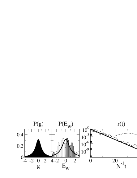
Figure 3: Same as Fig. 2 but for a Lorentzian distribution of the couplings ${g_{k}}$. In this case $r(t)$ decays exponentially. The histogram and the dashed line in $r(t)$ correspond to $N=20$, the straight thin line is a particular case for $N=100$ and the thick line is the average. We note that the convergence is slower than in the Gaussian case of Fig. 2, because realizations of ${g_{k}}$ are more likely to have one or two dominant couplings. Therefore, although the average shows a clear exponential decay, fluctuations are noticeable even for large $N$. Notice also that the logarithmic scale confirms the long time saturation of $r(t)$ at $\sim 2^{-N/2}$, Eq (7).

Possible experimental applications of our considerations are in nuclear magnetic resonance, but also in other situations where two-level systems interact with spin environments. We note that a Gaussian time dependence has been seen in the NMR setting DiffusionNMR but it is usually explained by spin diffusion models (which have rather different character and employ a different set of assumptions). Moreover, there is a substantial body of work Dobrovitski ; deRaedt ; Loss on decoherence due to spin environments, stimulated in part by the interests of quantum computation. The relation between the decoherence factor and the strength function might prove useful in the physical setting of strongly interacting fermions, where it has been shown that the strength function takes a Gaussian shape Kota . It is our hope that the simple analytic model described here will assist in gaining further insights into these fascinating problems.

We acknowledge fruitful discussions with R. Blume-Kohout and G. Raggio. We also acknowledge partial support from ARDA/NSA grant. JPP received also partial support from a grant by Fundación Antorchas.

References

- (1) W.H. Zurek, Phys. Rev. D 26, 1862 (1982)
- (2) W.H. Zurek, Phys. Today 44, 36 (1991); J. P. Paz and W. H. Zurek, in Coherent matter waves, Les Houches Session LXXII, R Kaiser, C Westbrook and F David eds., EDP Sciences (Springer Verlag, Berlin, 2001) 533-614; W.H. Zurek, Rev. Mod. Phys. 75, 715 (2003).
- (3) M. A. Nielsen and I. L. Chuang, Quantum computation and quantum information (Cambridge University Press, Cambridge, New York, 2000).
- (4) A. Kossakowski, Bull. Acad. Pol. Sci., Ser. Sci., Math. Astron. Phys. 21, 649 (1973); G. Lindblad, Commun. Math. Phys. 48, 119 (1976)
- (5) J. Preskill, Phys. Today 52 (6), 24 (1999).
- (6) B.V. Gnedenko, The Theory of Probability, Fourth edition (Chelsea, New York,1968), see Chap. VIII.
- (7) G.Casati, B.V. Chirikov, I. Guarneri and F.M. Izrailev, Phys. Rev. E 48 R1613 (1993); Phys. Lett. A 223, 430 (1996).
- (8) L. Breiman, Probability, Classics in Applied Mathematics (SIAM, Philadelphia, 1992).
- (9) F.M. Cucchietti, W.H. Zurek and J.P. Paz, in preparation.
- (10) V.V. Dobrovitski, H.A. De Raedt, M.I. Katsnelson and B.N. Harmon, quant-ph/0112053.
- (11) R.A. Jalabert and H.M. Pastawski, Phys. Rev. Lett. 86, 2490 (2001); Ph. Jacquod, P. G. Silvestrov, and C. W. J. Beenakker, Phys. Rev. E 64, 055203 (2001); F.M. Cucchietti, H.M. Pastawski, and R.A. Jalabert, cond-mat/0307752.
- (12) F.M. Cucchietti, D. A. R. Dalvit, J.P. Paz, and W. H. Zurek, Phys. Rev. Lett. 91, 210403 (2003).
- (13) E. Heller in Chaos and Quantum Physics, Proceedings of Session LII of the Les Houces Summer School, edited by A. Voros and M.J. Giannoni (North-Holland, Amsterdam, 1990).
- (14) A. Abragam, The principles of nuclear magnetism, Clarendon Press, Oxford (1978); T.T.P. Cheung, Phys. Rev. B 23, 1404 (1981).
- (15) V.V. Dobrovitski and H. A. De Raedt, Phys. Rev. E 67, 056702 (2003); H.A. De Raedt and V.V. Dobrovitski, quant-ph/0301121.
- (16) J. Schliemann, A.V. Khaetskii and D. Loss, Phys. Rev. B 66, 245303 (2002).
- (17) V.K.B. Kota, Phys. Rep. 347, 223 (2001); V.V. Flambaum and F.M. Izrailev, Phys. Rev. E 61, 2539 (2000).