Partial Wave Analysis of Scattering with Nonlocal Aharonov-Bohm Effect and Anomalous Cross Section Induced by Quantum Interference

Abstract

Partial wave theory of a three dmensional scattering problem for an arbitray short range potential and a nonlocal Aharonov-Bohm magnetic flux is established. The scattering process of a “hard shere” like potential and the magnetic flux is examined. An anomalous total cross section is revealed at the specific quantized magnetic flux at low energy which helps explain the composite fermion and boson model in the fractional quantum Hall effect. Since the nonlocal quantum interference of magnetic flux on the charged particles is universal, the nonlocal effect is expected to appear in quite general potential system and will be useful in understanding some other phenomena in mesoscopic phyiscs.

I Introduction

Since the global structure of magnetic flux was discovered about 40 years ago 1 , it had great contribution to our comprehension of the foundation of quantum theory 2 , the phenomenon of quantum Hall effect 3 , superconductivity 4 , repulsive Bose gases 6 , and, recently, help to explore the quantum computers, quantum cryptography communication systems 7 ; 8 . Nevertheless, to my knowledge, a general partial wave analysis for a scattering of a charged particle moving in an arbitrary short range potential plus a magnetic flux in three dimensions is still not done until now 8a . In this paper we discuss partial wave method of a charged particle moving in an arbitrary short range potential with scattering center located at the origin, and the AB magnetic flux along z-axis in the three dimensional space. Special attention is paid to the problem of the “hard sphere” like potential plus the magnetic flux with the incident direction of particles restricted in $x$-$y$ plane. Several interesting results are concluded as follows: (1) In the long wave length limit ( equivalently, short range potential) the total cross section is drastically suppressed at quantized magnetic flux $\Phi=(2n+1)\Phi_{0}/2,$ where $n=0,1,2,\cdots$, and $\Phi_{0}$ is the fundamental magnetic flux quantum $hc/e$. The global influence of the magnetic flux on the cross section is manifested with $\Phi_{0}$ periodicity. The result provides another possibility to explain the anomalous total cross section given in Ref. 9 , where the quantum entanglement is supposedly responsible for the suppression of total cross section in the condensed system. On the other hand, the cross section approaches the flux-free case in the short wave length limit, i.e. the quantum interference feature of the nonlocal effect gradually disappears, and the cross section approaches the classical limit. (2) If the hard sphere is used to simulate the boson (fermion) moving in $x$-$y$ plane, the scattering process of identical particles carrying the magnetic flux shows that the total cross section is suppressed at quantized magnetic flux $\Phi=(2n+1)\Phi_{0}$ for bosons ($\Phi=2n\Phi_{0}$ for fermions) and exhibits the global structure with $2\Phi_{0}$ periodicity. These results shed light on the model of composite bosons and fermions in the fractional quantum Hall effect 3 ; 11 ; 12 , superconductivity, and transport phenomena in nanostructures 13a ; 13b . Furthermore, since the nonlocal influence of the magnetic flux on the charged particle are universal, the implication should be general in similar systems.

This paper is organized as follows. In section II, the partial wave method of scattering with AB effect in three dimensions is established. The nonintegrable phase factor (NPF) 13 is used to couple the magnetic flux with the particle angular momentum such that the partial wave method can be conveniently developed. In section III, special attention is paid to the specific condition of the incident direction restricted in the $x$-$y$ plane. The total cross section of a charged particle with its path in $x$-$y$ plane scattered by a hard sphere potential plus an AB magnetic flux is discussed in some detail. Our discussions are summarized in section V.

II Partial Wave Analysis of Scattering With Nonlocal Aharonov-Bohm Effect

We consider a three-dimensional model. The fixed-energy Green’s function $G^{(0)}({\bf x,x}^{\prime};E)$ for a charged particle with mass $\mu$ propagating from ${\bf x}^{\prime}$ to ${\bf x}$ satisfies the Schrödinger equation

$$\left\{E-\left[-\frac{\hbar^{2}\nabla^{2}}{2\mu}+V({\bf x})\right]\right\}G^{(0)}({\bf x,x}^{\prime};E)=\delta({\bf x-x}^{\prime}),$$ (1)

where $V({\bf x})$ is the scalar potential and ${\bf x}$ is the three dimensional coordinate vector. In the spherically symmetric system, the Green’s function can be decomposed as 13c

$$G^{(0)}({\bf r,r}^{\prime};E)=\sum_{l=0}^{\infty}\sum_{m=-l}^{l}G_{l}^{(0)}(r{\bf,}r^{\prime};E)Y_{lm}(\theta,\varphi)Y_{lm}^{\ast}(\theta^{\prime},\varphi^{\prime})$$ (2)

with $Y_{lm}(\theta,\varphi)$ the well-known spherical harmonics and $G_{l}^{(0)}(r{\bf,}r^{\prime};E)$ the radial Green’s function for the specific angular momentum channel $l$. The left-hand side of Eq. (1) can then be cast into

$$\sum_{l=0}^{\infty}\sum_{m=-l}^{l}\left\{E+\left[\frac{\hbar^{2}}{2\mu}\left(\frac{d^{2}}{dr^{2}}+\frac{2}{r}\frac{d}{dr}\right)-\frac{l(l+1)\hbar^{2}}{2\mu r^{2}}\right]-V(r)\right\}$$

$$\times G_{l}^{(0)}(r{\bf,}r^{\prime};E)Y_{lm}(\theta,\varphi)Y_{lm}^{\ast}(\theta^{\prime},\varphi^{\prime}).$$ (3)

For a charged particle affected by a magnetic field, the Green’s function $G({\bf x,x}^{\prime};E)$ is different from $G^{(0)}({\bf x,x}^{\prime};E)$ by a global NPF 13 ; 13c ; 14 ; 15 ; 16 ; 17 ; 18

$$G({\bf x},{\bf x}^{\prime};E)=G^{(0)}({\bf x},{\bf x}^{\prime};E)\exp\left\{\frac{ie}{\hbar c}\int_{{\bf x}^{\prime}}^{{\bf x}}{\bf A(\tilde{x}})\cdot d{\bf\tilde{x}}\right\}.$$ (4)

Here the vector potential ${\bf A(x})$ is used to represent the magnetic field. For an infinitely thin tube of finite magnetic flux along the $z$-direction, the vector potential can be described by

$${\bf A(x})=2g\frac{-y{\hat{e}}_{x}+x{\hat{e}}_{y}}{x^{2}+y^{2}},$$ (5)

where ${\hat{e}}_{x},{\hat{e}}_{y}$ stand for the unit vector along the $x,y$ axis respectively. Introducing the azimuthal angle $\varphi({\bf x})=\tan^{-1}(y/x)$ around the AB tube, the components of the vector potential can be expressed as $A_{i}=2g\partial_{i}\varphi({\bf x}).$ The associated magnetic field lines are confined to an infinitely thin tube along the $z$-axis,

$$B_{3}=2g\epsilon_{3ij}\partial_{i}\partial_{j}\varphi({\bf x})=4\pi g\delta({\bf x}_{\bot}),$$ (6)

where ${\bf x}_{\bot}$ stands for the transverse vector ${\bf x}_{\bot}\equiv(x,y).$ Since the magnetic flux through the tube is defined by the integral $\Phi=\int d^{2}xB_{3}$, the coupling constant $g$ is related to the magnetic flux by $g=\Phi/4\pi$. By using the expression of $A_{i}=2g\partial_{i}\varphi$, the angular difference between the initial point ${\bf x}^{\prime}$ and the final point ${\bf x}$ in the exponent of the NPF is given by

$$\varphi-\varphi^{\prime}=\int_{t}^{t^{\prime}}d\tau\dot{\varphi}(\tau)=\int_{t}^{t^{\prime}}d\tau\frac{-y\dot{x}+x\dot{y}}{x^{2}+y^{2}}=\int_{{\bf x}^{\prime}}^{{\bf x}}\frac{{\bf\tilde{x}\times}d{\bf\tilde{x}}}{{\bf\tilde{x}}^{2}},$$ (7)

where $\dot{\varphi}=d\varphi/d\tau$. Given two paths $C_{1}$ and $C_{2}$ connecting ${\bf x}^{\prime}$ and ${\bf x}$, the integral differs by an integer multiple of $2\pi$. The winding number is thus given by the contour integral over the closed difference path $C$:

$$n=\frac{1}{2\pi}\oint_{C}\frac{{\bf\tilde{x}\times}d{\bf\tilde{x}}}{{\bf\tilde{x}}^{2}}.$$ (8)

The magnetic interaction is therefore purely nonlocal and topological 18a . Its action takes the form ${\cal A}_{{\rm mag}}=-\hbar\mu_{0}2\pi n,$ where $\mu_{0}\equiv-2eg/\hbar c=-\Phi/\Phi_{0}$ is a dimensionless number with the customarily minus sign. The NPF now becomes $\exp\left\{-i\mu_{0}(2\pi n+\varphi-\varphi^{\prime})\right\}$. With the help of the equality between the associated Legendre polynomial $P_{l}^{m}(z)$ and the Jacobi function $P_{n}^{\left(\alpha,\beta\right)}(z)$ 17 ; 18 ,

$$P_{l}^{m}(\cos\theta)=(-1)^{m}\frac{\Gamma(l+m+1)}{\Gamma(m+1)}\left(\cos\frac{\theta}{2}\sin\frac{\theta}{2}\right)^{m}P_{l-m}^{\left(m,m\right)}(\cos\theta),$$ (9)

the angular part of the Green’s function in the expression (2) can be turned into the following form

$$\sum_{m{\bf=-}l}^{l}Y_{lm}(\theta,\varphi)Y_{lm}^{\ast}(\theta^{\prime},\varphi^{\prime})=\sum_{m{\bf=-}l}^{l}\frac{2l+1}{4\pi}\frac{\Gamma\left(l-m+1\right)}{\Gamma\left(l+m+1\right)}P_{l}^{m}(\cos\theta)P_{l}^{m}(\cos\theta^{\prime})e^{im(\varphi-\varphi^{\prime})}$$

$$=\sum_{m{\bf=-}l}^{l}\left[\frac{2l+1}{4\pi}\frac{\Gamma\left(l-m+1\right)\Gamma\left(l+m+1\right)}{\Gamma^{2}\left(l+1\right)}\right]\left(\cos\frac{\theta}{2}\cos\frac{\theta^{\prime}}{2}\sin\frac{\theta}{2}\sin\frac{\theta^{\prime}}{2}\right)^{m}$$

$$\times P_{l-m}^{\left(m,m\right)}(\cos\theta)P_{l-m}^{\left(m,m\right)}(\cos\theta^{\prime})e^{im\left(\varphi-\varphi^{\prime}\right)}.$$ (10)

In order to include the NPF due to the AB effect, we will change the index $l$ into $q$ related by the definition $l-m=q$. As a result Eq. (3) can be rewritten as

$$\sum_{q=0}^{\infty}\sum_{m=-\infty}^{\infty}\left\{E+\left[\frac{\hbar^{2}}{2\mu}\left(\frac{d^{2}}{dr^{2}}+\frac{2}{r}\frac{d}{dr}\right)-\frac{(q+m)(q+m+1)\hbar^{2}}{2\mu r^{2}}\right]-V(r)\right\}$$

$$\times G_{q+m}^{(0)}(r{\bf,}r^{\prime};E)\left[\frac{2(q+m)+1}{4\pi}\frac{\Gamma\left(q+1\right)\Gamma\left(q+2m+1\right)}{\Gamma^{2}\left(q+m+1\right)}\right]\left(\cos\frac{\theta}{2}\cos\frac{\theta^{\prime}}{2}\sin\frac{\theta}{2}\sin\frac{\theta^{\prime}}{2}\right)^{m}$$

$$\times P_{q}^{\left(m,m\right)}(\cos\theta)P_{q}^{\left(m,m\right)}(\cos\theta^{\prime})e^{im\left(\varphi-\varphi^{\prime}\right)}.$$ (11)

The Green’s function $G_{n}(r,r^{\prime};E)$ for a specific winding number $n$ can be obtained by converting the summation over $m$ in Eq. (11) into an integral over $z$ and another summation over $n$ by the Poisson’s summation formula (e.g. Ref. 19 p.469)

$$\sum_{m=-\infty}^{\infty}f(m)=\int_{-\infty}^{\infty}dz\sum_{n=-\infty}^{\infty}e^{2\pi nzi}f(z).$$ (12)

So the expression (3) when includes the NPF can be written as

$$\sum_{q=0}^{\infty}\int dz\sum_{n=-\infty}^{\infty}\left\{E+\left[\frac{\hbar^{2}}{2\mu}\left(\frac{d^{2}}{dr^{2}}+\frac{2}{r}\frac{d}{dr}\right)+\frac{(q+z)(q+z+1)\hbar^{2}}{2\mu r^{2}}\right]-V(r)\right\}$$

$$\times G_{q+z}(r{\bf,}r^{\prime};E)\left[\frac{2(q+z)+1}{4\pi}\frac{\Gamma\left(q+1\right)\Gamma\left(q+2z+1\right)}{\Gamma^{2}\left(q+z+1\right)}\right]\left(\cos\frac{\theta}{2}\cos\frac{\theta^{\prime}}{2}\sin\frac{\theta}{2}\sin\frac{\theta^{\prime}}{2}\right)^{z}$$

$$\times P_{q}^{\left(z,z\right)}(\cos\theta)P_{q}^{\left(z,z\right)}(\cos\theta^{\prime})e^{i(z-\mu_{0})\left(\varphi+2n\pi-\varphi^{\prime}\right)},$$ (13)

where the superscript $(0)$ in $G_{q+m}^{(0)}$ has been suppressed to denote that the AB effect is included. Obviously, the number $n$ in the right-hand side is precisely the winding number by which we want to classify the Green’s function. Employing the special case of the Poisson formula $\sum_{n=-\infty}^{\infty}\exp\{ik(\varphi+2n\pi-\varphi^{\prime})\}=\sum_{m=-\infty}^{\infty}\delta(k-m)\exp\{im(\varphi-\varphi^{\prime})\},$ the summation over all indices $n$ forces $z=\mu_{0}$ modulo an arbitrary integer number. Thus, we obtain

$$\sum_{q=0}^{\infty}\sum_{m=-\infty}^{\infty}\left\{E+\left[\frac{\hbar^{2}}{2\mu}\left(\frac{d^{2}}{dr^{2}}+\frac{2}{r}\frac{d}{dr}\right)-\frac{(q+\left|m+\mu_{0}\right|)(q+\left|m+\mu_{0}\right|+1)\hbar^{2}}{2\mu r^{2}}\right]-V(r)\right\}$$

$$\times G_{q+\left|m+\mu_{0}\right|}(r{\bf,}r^{\prime};E)\left\{\frac{\left[2\left(q+\left|m+\mu_{0}\right|\right)+1\right]}{4\pi}\frac{\Gamma\left(q+1\right)\Gamma\left(2\left|m+\mu_{0}\right|+q+1\right)}{\Gamma^{2}\left(\left|m+\mu_{0}\right|+q+1\right)}\right\}e^{im\left(\varphi-\varphi^{\prime}\right)}$$

$$\times\left(\cos\frac{\theta}{2}\cos\frac{\theta^{\prime}}{2}\sin\frac{\theta}{2}\sin\frac{\theta^{\prime}}{2}\right)^{\left|m+\mu_{0}\right|}P_{q}^{\left(\left|m+\mu_{0}\right|,\left|m+\mu_{0}\right|\right)}(\cos\theta)P_{q}^{\left(\left|m+\mu_{0}\right|,\left|m+\mu_{0}\right|\right)}(\cos\theta^{\prime}).$$ (14)

We see that the influence of the AB effect to the radial Green’s function is to replace the integer quantum number $l$ with a real one $(q+\left|m+\mu_{0}\right|)$ which depends on the magnitude of magnetic flux. Analogously the same procedure can be applied to the delta function $\delta({\bf r-r}^{\prime})$ in the  r.h.s. of Eq. (1) by employing the solid angle representation of the $\delta$ function

$$\delta\left(\Omega-\Omega^{\prime}\right)=\sum_{l=0}^{\infty}\sum_{m=-l}^{l}Y_{lm}(\theta,\varphi)Y_{lm}^{\ast}(\theta^{\prime},\varphi^{\prime}).$$ (15)

With the help of orthogonal property of the angular part 18 ,

$$\int_{0}^{2\pi}d\varphi\int_{-1}^{1}(d\cos\theta)P_{q}^{\left(\left|m+\mu_{0}\right|,\left|m+\mu_{0}\right|\right)}(\cos\theta)P_{q^{\prime}}^{\left(\left|m^{\prime}+\mu_{0}\right|,\left|m^{\prime}+\mu_{0}\right|\right)}(\cos\theta)$$

$$\left(\cos\frac{\theta}{2}\sin\frac{\theta}{2}\right)^{\left|m+\mu_{0}\right|}\left(\cos\frac{\theta}{2}\sin\frac{\theta}{2}\right)^{\left|m^{\prime}+\mu_{0}\right|}e^{i(m-m^{\prime})\varphi}$$

$$=\frac{\Gamma^{2}\left(q+\left|m+\mu_{0}\right|+1\right)}{\Gamma\left(q+1\right)\Gamma\left(q+2\left|m+\mu_{0}\right|+1\right)}\frac{4\pi}{2\left(q+\left|m+\mu_{0}\right|\right)+1}\delta_{q,q^{\prime}}\delta_{m,m^{\prime}},$$ (16)

one can show that the radial Green’s function for the set of the fixed quantum numbers $(q,m)$ satisfies

$$\left\{E+\left[\frac{\hbar^{2}}{2\mu}\left(\frac{d^{2}}{dr^{2}}+\frac{2}{r}\frac{d}{dr}\right)-\frac{\alpha(\alpha+1)\hbar^{2}}{2\mu r^{2}}\right]-V(r)\right\}$$

$$\times G_{\alpha}(r{\bf,}r^{\prime};E)=\delta(r{\bf-}r^{\prime}).$$ (17)

Here we have defined $\alpha\equiv(q+\left|m+\mu_{0}\right|)$ for convenience. The corresponding radial wave equation then reads

$$\left[\frac{d^{2}}{dr^{2}}+\frac{2}{r}\frac{d}{dr}+\left(k^{2}-U(r)-\frac{\alpha(\alpha+1)}{r^{2}}\right)\right]R_{k\alpha}(r)=0,$$ (18)

where $U(r)\equiv 2\mu V(r)/\hbar^{2}$ and the subscript set $(k,\alpha)$ with $k\equiv\sqrt{2\mu E}/\hbar$ in the radial wave function $R_{k\alpha}(r)$ denotes the state of scattering particle. For a short range potential, say $V(r)$ vanishes as $r>a$, the exterior solution is the linear combination of 1st and 2nd kind spherical Bessel functions $j_{\alpha}(kr)$, and $n_{\alpha}(kr)$, and may be given by

$$R_{\alpha k}(r)=\left[C_{\alpha}(k)j_{\alpha}(kr)+D_{\alpha}(k)n_{\alpha}(kr)\right]$$

$$=A_{\alpha}(k)\left[\cos\delta_{\alpha}(k)j_{\alpha}(kr)-\sin\delta_{\alpha}(k)n_{\alpha}(kr)\right],$$ (19)

where $\delta_{\alpha}(k)$ is the phase shift defined by $-D_{\alpha}(k)/C_{\alpha}(k)\equiv\tan\delta_{\alpha}(k)$ and $A_{\alpha}(k)=$ $C_{\alpha}(k)/\cos\delta_{\alpha}(k)$ which can be used to measure the interaction strength of potential. Thus the general solution $\Psi_{{\bf k}}({\bf x})$ of a scattering particle with arbitrary incident direction $(\theta^{\prime},\varphi^{\prime})$ is given by superposition of partial waves $\Psi_{k\alpha}(r)$, which reads

$$\Psi_{{\bf k}}({\bf x})=\sum_{q=0}^{\infty}\sum_{m=-\infty}^{\infty}A_{\alpha}(k)\left[\cos\delta_{\alpha}(k)j_{\alpha}(kr)-\sin\delta_{\alpha}(k)n_{\alpha}(kr)\right]{\cal Y}_{qm}^{\ast}(\theta^{\prime},\varphi^{\prime}){\cal Y}_{qm}(\theta,\varphi)$$ (20)

in which ${\cal Y}_{qm}(\theta,\varphi)$ is defined by

$${\cal Y}_{qm}(\theta,\varphi)=\sqrt{\frac{\Gamma(q+1)\Gamma(\alpha+\left|m+\mu_{0}\right|+1)}{\Gamma^{2}(\alpha+1)}}$$

$$\times\left(\cos\frac{\theta}{2}\sin\frac{\theta}{2}\right)^{\left|m+\mu_{0}\right|}P_{q}^{(\left|m+\mu_{0}\right|,\left|m+\mu_{0}\right|)}(\cos\theta)e^{im\varphi}.$$ (21)

Since it must describe both the incident and the scattered waves at large distance, we naturally expect it to become

$$\Psi_{{\bf k}}({\bf x})\stackrel{{\scriptstyle\left|{\bf x}\right|\rightarrow\infty}}{{\longrightarrow}}{\cal F}_{\infty}\left(\exp\{i{\bf k\cdot x}\}\exp\left\{\frac{ie}{\hbar c}\int_{C}^{{\bf x}}{\bf A(\tilde{x}})\cdot d{\bf\tilde{x}}\right\}\right)+f(\theta,\varphi)\frac{\exp\{ikr\}}{r},$$ (22)

where $\exp\{i{\bf k\cdot x}\}$ describes the incident plane wave of a charged particle with momentum ${\bf p}=\mu{\bf k}$ and ${\cal F}_{\infty}(\cdot)$ stands for its asymptotic form. The phase modulation of the NPF comes from the fact that the field ${\bf A(x})$ of AB magnetic flux affects the charged particle globally. The subscript $C$ in the integral is used to represent the nature of the NPF which depends on the different paths. To find the amplitude $f(\theta,\varphi)$ we first note that the plane wave in Eq. (22) can be expanded in terms of the spherical harmonics

$$e^{i{\bf k\cdot x}}=\sum_{l=0}^{\infty}\sum_{m=-l}^{l}4\pi i^{l}j_{l}(kr)Y_{lm}^{\ast}(\theta^{\prime},\varphi^{\prime})Y_{lm}(\theta,\varphi).$$ (23)

The parameters ${\bf(}k,\theta^{\prime},\varphi^{\prime})$ and ${\bf(}r,\theta,\varphi)$ denote the corresponding components of ${\bf k}$ and ${\bf r}$ in spherical coordinates respectively. Using the same procedure as in Eqs. (10)$\sim$(14), we combine the nonlocal flux effect into the partial wave expansion, and obtain the result

$$e^{i{\bf k\cdot x}}e^{\frac{ie}{\hbar c}\int_{C}^{{\bf x}}{\bf A(\tilde{x}})\cdot d{\bf\tilde{x}}}=\sum_{q=0}^{\infty}\sum_{m=-\infty}^{\infty}(2\alpha+1)i^{\alpha}j_{\alpha}(kr){\cal Y}_{qm}^{\ast}(\theta^{\prime},\varphi^{\prime}){\cal Y}_{qm}(\theta,\varphi).$$ (24)

By employing approximations of spherical Bessel functions [see Eq. (42)],

$$j_{\alpha}(kr)\stackrel{{\scriptstyle r\rightarrow\infty}}{{\longrightarrow}}\frac{1}{kr}\sin(kr-\alpha\pi/2),$$ (25)

$$n_{\alpha}(kr)\stackrel{{\scriptstyle r\rightarrow\infty}}{{\longrightarrow}}-\frac{1}{kr}\cos(\alpha\pi)\cos(kr+\alpha\pi/2),$$ (26)

we can find that

$$R_{\alpha k}(r)\stackrel{{\scriptstyle r\rightarrow\infty}}{{\longrightarrow}}\frac{A_{\alpha}(k)}{kr}\left\{\sin\left[kr-\alpha\pi/2+\delta_{\alpha}(k)\right]-\sin(\alpha\pi)\sin\delta_{\alpha}(k)\sin(kr+\alpha\pi/2)\right\}.$$ (27)

Substituting the result for $R_{\alpha k}(r)$ in (20), and comparing both asymptotic forms of (20) and (22), the scattering amplitude is found to be

$$f(\theta,\varphi)=\frac{1}{k}\sum_{q=0}^{\infty}\sum_{m=-\infty}^{\infty}\left(2\alpha+1\right)\left[\frac{e^{i\delta_{\alpha}}\sin\delta_{\alpha}\cos^{2}(\alpha\pi)}{1-e^{i(\delta_{\alpha}-\alpha\pi)}\sin\delta_{\alpha}\sin(\alpha\pi)}\right]{\cal Y}_{qm}^{\ast}(\theta^{\prime},\varphi^{\prime}){\cal Y}_{qm}(\theta,\varphi).$$ (28)

Here $(\theta^{\prime},\varphi^{\prime})$ is the incident direction of a charged particle, and $(\theta,\varphi)$ is the scattering direction. It is easy to see that when the magnetic flux disappears, with $\theta^{\prime}=0$, i.e. ${\bf k}$ is along the z-axis, and $P_{l}(1)=1$, the result reduces to the well-known amplitude

$$f(\theta)=\frac{1}{k}\sum_{l=0}^{\infty}\left(2l+1\right)e^{i\delta_{l}}\sin\delta_{l}P_{l}(\cos\theta)$$ (29)

Let us consider the case of the incident direction perpendicular to the magnetic flux, i.e. $(\theta^{\prime}=\pi/2,\varphi^{\prime}=0)$. We have the function

$${\cal Y}_{qm}(\pi/2,0)=\sqrt{\frac{\Gamma(q+1)\Gamma(\alpha+\left|m+\mu_{0}\right|+1)}{\Gamma^{2}(\alpha+1)}}\left(\frac{1}{2}\right)^{\left|m+\mu_{0}\right|}P_{q}^{(\left|m+\mu_{0}\right|,\left|m+\mu_{0}\right|)}(0).$$ (30)

With the help of the formulas (p.218$\sim$219 19 )

$$P_{q}^{(\beta,\beta)}(z)=\frac{\Gamma(2\beta+1)\Gamma(q+\beta+1)}{\Gamma(\beta+1)\Gamma(q+2\beta+1)}C_{q}^{\beta+1/2}(z),$$ (31)

$$C_{q}^{\beta+1/2}(0)=\left\{\begin{array}[]{l}0\text{ \ if \ }q=\text{odd numbers}\\ (-1)^{\tilde{q}}\frac{\Gamma(\tilde{q}+\beta+1/2)}{\Gamma(\beta+1/2)\Gamma(\tilde{q}+1)}\text{ if }q=\text{even numbers}\end{array}\right.,$$ (32)

here $\tilde{q}\equiv q/2=0,1,2,\cdots$, and $C_{q}^{\beta+1/2}(z)$ is the Gegenbauer polynomials, we can find that $P_{q}^{(\beta,\beta)}(0)=0$ if $q=$odd numbers, and

$$P_{q}^{(\beta,\beta)}(0)$$

$$=(-1)^{\tilde{q}}\frac{\Gamma(2\beta+1)\Gamma(2\tilde{q}+\beta+1)\Gamma(\tilde{q}+\beta+1/2)}{\Gamma(\beta+1)\Gamma(2\tilde{q}+2\beta+1)\Gamma(\beta+1/2)\Gamma(\tilde{q}+1)},\text{ if\ }q=\text{even numbers,}$$ (33)

where $\beta\equiv\left|m+\mu_{0}\right|$. Thus the function ${\cal Y}_{qm}(\pi/2,0)$ is given by

$${\cal Y}_{qm}(\pi/2,0)=(-1)^{\tilde{q}}\frac{1}{\sqrt{\pi}}\sqrt{\frac{\Gamma(\tilde{q}+1/2)\Gamma(\tilde{q}+\beta+1/2)}{\Gamma(\tilde{q}+\beta+1)\Gamma(\tilde{q}+1)}}.$$ (34)

In most cases, the total cross section of our major concern is defined by $\sigma_{t}=\int\sigma(\theta,\varphi)d\Omega$, where $d\Omega$ is the solid angle. By employing (16), the partial wave representation of total cross section for a charged particle scattered by a short range potential plus the nonlocal AB effect is given by

$$\sigma_{t}=\frac{4\pi}{k^{2}}\sum_{\tilde{q}=0}^{\infty}\sum_{m=-\infty}^{\infty}F_{\tilde{q}m}(\delta_{\tilde{\alpha}})$$ (35)

with

$$F_{\tilde{q}m}(\delta_{\tilde{\alpha}})=\left[\frac{(2\tilde{\alpha}+1)\sin^{2}\delta_{\tilde{\alpha}}\cos^{4}(\tilde{\alpha}\pi){\cal Y}_{\tilde{q}m}^{2}}{1-2\sin\delta_{\tilde{\alpha}}\sin(\tilde{\alpha}\pi)\cos(\tilde{\alpha}\pi-\delta_{\tilde{\alpha}})+\sin^{2}\delta_{\tilde{\alpha}}\sin^{2}(\tilde{\alpha}\pi)}\right],$$

where we have defined $\tilde{\alpha}\equiv(2\tilde{q}+\beta)$, and

$${\cal Y}_{\tilde{q}m}^{2}\equiv\frac{\Gamma\left(\tilde{q}+1/2\right)\Gamma(\tilde{q}+\beta+1/2)}{\left[\pi\Gamma\left(\tilde{q}+1\right)\Gamma(\tilde{q}+\beta+1)\right]}.$$ (36)

It is obvious that the cross section is completely determined by the scattering phase shifts which are concluded by the potential of different types. Furthermore, when a nonlocal AB magnetic flux exists, both the phase shift and the cross section are affected globally. A relation between the total cross section $\sigma_{t}$ and the scattering amplitude is obtained if we set $\varphi=0$, and then take the imaginary part. It gives $\sigma_{t}=\left(4\pi/k\right)\mathop{\rm Im}f(\theta=\pi/2,\varphi=0)$. This is the optical theorem and is essentially a consequence of the conservation of particles. For the scattering of identical bosons (fermions) carrying the magnetic flux, the differential cross section is given by $\sigma(\theta,\varphi)=\left|f(\theta,\varphi)\pm f(\pi-\theta,\varphi+\pi)\right|^{2}$, where the plus sign is for bosons as usual. The total cross sections are given by the integral $\int_{-\pi}^{\pi}\sigma(\theta,\varphi)d\Omega$, which yield

$$\sigma_{t}({\rm bosons})=\frac{16\pi}{k^{2}}\sum_{\tilde{q}=0}^{\infty}\sum_{m=-\infty,{\rm even}}^{\infty}F_{\tilde{q}m}(\delta_{\tilde{\alpha}}),$$ (37)

and

$$\sigma_{t}({\rm fermions})=\frac{16\pi}{k^{2}}\sum_{\tilde{q}=0}^{\infty}\sum_{m=-\infty,{\rm odd}}^{\infty}F_{\tilde{q}m}(\delta_{\tilde{\alpha}}).$$ (38)

Here the subscript “odd” (“even”) is used to indicate the summation over odd (even) numbers only.

III Anomalous Cross Section induced by Quantum Interference

As a realization of the nonlocal influence of the AB flux on the cross section, let us consider a charged particle scattered by a hard sphere potential and a magnetic flux. The potential is given by $V(r)=\infty,$ for $r\leq a$, and $V(r)=0,$ for $r\leq a$. Using the boundary condition of the wave function $R_{k\alpha}(a^{+})=0$, we find that the phase shift is given by

$$\tan\delta_{\tilde{\alpha}}=j_{\tilde{\alpha}}(ka)/n_{\tilde{\alpha}}(ka).$$ (39)

Substituting this expression into (35), the total cross section is found to be

$$\sigma_{t}=\frac{4\pi}{k^{2}}\sum_{\tilde{q}=0}^{\infty}\sum_{m=-\infty}^{\infty}\frac{(2\tilde{\alpha}+1)\cos^{2}(\tilde{\alpha}\pi)J_{\tilde{\alpha}+1/2}^{2}(ka){\cal Y}_{\tilde{q}m}^{2}}{J_{{}_{\tilde{\alpha}+1/2}}^{2}(ka)+J_{{}_{-\tilde{\alpha}-1/2}}^{2}(ka)+2\sin(\tilde{\alpha}\pi)J_{\tilde{\alpha}+1/2}(ka)J_{{}_{-\tilde{\alpha}-1/2}}(ka)}.$$ (40)

To obtain the result, we have applied the following relations between the Bessel functions and spherical Bessel functions

$$j_{\nu}(z)=\sqrt{\frac{\pi}{2z}}J_{\nu+1/2}(z),$$ (41)

and

$$n_{\nu}(z)=\left[\cos(\nu+1)\pi\right]\sqrt{\frac{\pi}{2z}}J_{-\nu-1/2}(z).$$ (42)

The asymptotic behavior in (26) can be found by the equality. Note that the result will reduce to the pure hard sphere case

$$\sigma_{t}=\frac{4\pi}{k^{2}}\sum_{l=0}^{\infty}\frac{(2l+1)j_{l}^{2}(ka)}{j_{l}^{2}(ka)+n_{l}^{2}(ka)}$$ (43)

if the flux disappears, i.e. $\mu_{0}=0$. In this case the low energy limit $k\rightarrow 0$ (assuming the radius $a$ is finite) of phase shift can be found by the asymptotic expansion of Bessel functions, which yields

$$\tan\delta_{l}=j_{l}(ka)/n_{l}(ka)\stackrel{{\scriptstyle k\rightarrow 0}}{{\longrightarrow}}-\frac{(ka)^{2l+1}}{[(2l-1)!!]^{2}(2l+1)}.$$ (44)

Obviously, only index $l=0$ survives. The phase shift becomes

$$\tan\delta_{0}(k)=j_{0}(ka)/n_{0}(ka)\approx-ka<0.$$ (45)

So the total cross section

$$\sigma_{t}\approx\frac{4\pi}{k^{2}}\sin^{2}\delta_{0}\approx\frac{4\pi}{k^{2}}\delta_{0}^{2}\approx 4\pi a^{2}.$$ (46)

At the high energy limit $k\rightarrow\infty$, we may use the formulas of spherical Bessel functions of the large argument to turn Eq. (43) into

$$\sigma_{t}\approx\frac{4\pi}{k^{2}}\sum_{l=0}^{[ka]}(2l+1)\sin^{2}(ka-l\pi/2)$$

$$=\lim_{ka\rightarrow\infty}\frac{4\pi}{k^{2}}\left\{\sum_{l=0,2,\cdots}^{[ka]}(2l+1)\sin^{2}\left(ka\right)+\sum_{l=1,3,\cdots}^{[ka]}(2l+1)\cos^{2}\left(ka\right)\right\}$$

$$=\lim_{ka\rightarrow\infty}\frac{4\pi}{k^{2}}\left\{\frac{ka(ka+1)}{2}\sin^{2}\left(ka\right)+\frac{(ka-1)(ka+2)}{2}\cos^{2}\left(ka\right)\right\}\approx 2\pi a^{2}.$$ (47)

The numerical result for $\alpha$ with noninteger value is plotted in Fig. 1, where the normalization $\sigma_{0}$ is chosen as $2\pi a^{2}$. There are two main results which are caused by the quantum interference of the AB effect: (1) The cross section $\sigma_{t}$ is drastically suppressed at the low energy limit (equivalently, the short range potential), say $ka\leq 1$, at quantized magnetic flux $\Phi=(2n+1)\Phi_{0}/2$, $n=0,1,2,\cdots$, with $\Phi_{0}$ periodicity as shown in Fig. 1 and Fig. 2. (2) A more interesting consideration is given by the scattering of identical particles simulated by the hard spheres carrying the magnetic flux. In Fig. 3, we plot the total cross sections of identical bosons carrying the magnetic flux via Eq. (37). The outcome shows that the cross section approaches zero ($\sigma_{t}\rightarrow 0$) when the value $ka\rightarrow 0$ if the magnetic flux is at quantized value $(2n+1)\Phi_{0}$. On the contrary, if the magnetic flux is equal to $2n\Phi_{0}$, the cross section becomes maximum and the effect of magnetic flux disappears. Since the decay rate of a current ${\bf j}$ traveling a distance ${\bf x}$ is given by ${\bf j(x)=j(}0{\bf)}\exp(-\sigma_{t}n_{0}{\bf x})$, where $n_{0}$ is the number of the scattering center, the total cross section $\sigma_{t}\rightarrow 0$ at the low energy limit at $\Phi=(2n+1)\Phi_{0}$ means that the resistance $R\rightarrow 0$ and results in the persistence of current. This phenomenon is consistent with the picture of composite boson in fractional quantum Hall states located at the filling factor with odd denominator such as $\nu=1/3$. The composite boson is pictured by an electron carrying the quantized magnetic flux $\Phi=(2n+1)\Phi_{0}$. It dictates the quantized Hall states which exhibit the perfect conduction in the longitudinal direction, i.e. the resistance originated from the collisions between composite bosons disappear 3 . The global structure of the total cross section is given by $2\Phi_{0}$ periodicity as shown in Fig. 4. In the case of identical fermions, the total cross section $\sigma_{t}\rightarrow 0$ is found at the quantized magnetic flux $\Phi=2n\Phi_{0}$ as shown in Fig. 5. Such effect is consistent with the model of composite fermion in the quantum Hall state located at the filling factor with even denominator $\nu=5/2$. The composite fermion is described by an electron carrying the quantized magnetic flux $\Phi=2n\Phi_{0}$. In Ref. 21 , a quantitative explanation of quantum Hall state at the filling factor $\nu=5/2$ is given by the existence of a shorter range potential between the composite fermions than the case of the filling factor $\nu=1/2$. Here we can see that, in Fig. 5, a sufficiently short range potential, say $ka<0.5$, between the fermions carrying the quantized magnetic flux $\Phi=2n\Phi_{0}$ will cause negligible cross section and thus agree with the composite fermions model. Similar to the boson case, the oscillating period is given by $2\Phi_{0}$ as shown in Fig. 6.

IV Discussion

1. Symmetries

When the incident direction is perpendicular to the magnetic flux,i.e. $(\theta^{\prime}=\pi/2,\varphi^{\prime}=0)$, we see from (32) that $q$ must be equal to even numbers so that these channels have nonvanishing contributions. In this case we have

$$P_{2\tilde{q}}^{(\beta,\beta)}(\cos(\pi-\theta))=P_{2\tilde{q}}^{(\beta,\beta)}(\cos\theta).$$ (48)

On the other hand, from (21) we have

$${\cal Y}_{qm}(\pi-\theta,\varphi)={\cal Y}_{qm}(\theta,\varphi).$$ (49)

These two equalities give us the relation in (28)

$$f(\theta,\varphi)=f(\pi-\theta,\varphi)$$ (50)

which means that the amplitude, and thus the cross section, is symmetric about the $x$-$y$ plane. If we make the condition $\varphi\rightarrow-\varphi,$ which is equivalent to $m\rightarrow-m$, the effect is equal to reverse the direction of flux form $+z$ to $-z$ since $\left|m+\mu_{0}\right|\rightarrow\left|-m+\mu_{0}\right|=\left|m-\mu_{0}\right|$.

2. Anomalous Cross Section Induced by the Quantum Interference

By way of Fig. 1, we see that the total cross section may be anomalous due to the quantum interference which provides another possibility to explain the depression of the total cross section discussed in recent papers 9 , where the quantum entanglement is supposedly responsible for the suppression of total cross section in the condensed matter. However, issues do exist regarding that the lifetime of the entanglement in condensed system is much shorter than the present-day time-resolution techniques can resolve, and therefore it is commonly expected to have no experimental significance.

3. The effects of magnetic flux and dimensions

The quantum interference features in Fig. 1$\sim$Fig. 6 were observed in 23 where a two dimensional partial wave analysis of scattering with nonlocal AB effect was constructed, and a “hard disk” with the AB magnetic flux was used to simulate the dynamics of a charged particle with magnetic flux. Although the dominate picture of the quantum interference can be found in the hard disk model, it is somewhat too simple to yield a “wave packet like” object. In the paper, with the hard sphere model, we see from Fig. 1$\sim$Fig. 6 that quantum interference features at the quantized magnetic flux $\Phi=(2n+1)\Phi_{0}/2$, $2n\Phi_{0}$, and $(2n+1)\Phi_{0}$ are apparent.

4. Extension the potential to more general case

Although in the procedure of our proof we assume $V(r)=0$ for $r>a$, we do not specify the radius $a$ beyond which $V(r)=0$. Hence we expect that the theorem given in the article should be valid for a very general potential as long as the potential decrease rapidly enough when $r\rightarrow\infty$.

5. A possible experimental test

In Ref. 22 , a general fractional (non-quantized) magnetic flux is observed in the superconducting film. Because of the inevitable pinning of flux in superconductor, the flux finally attaches to the defect or impurity such that they become models of a finite range interaction with flux as mentioned in point 4. The system scattered by the other low energy charged particle can be as the test ground of the anomalous cross section presented in the paper.

ACKNOWLEDGMENTS

The author would like to thank professor Pi-Guan Luan for helpful discussions, Professors Der-San Chuu, and Jang-Yu Hsu for reading the manuscript.

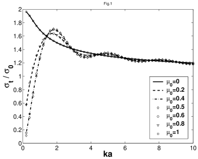
Figure 1: The total cross section for a charged particle scattered by a hard sphere with radius $a$ and a magnetic flux along the z-axis. The normalization $\sigma_{0}=2\pi a^{2}$ has been selected. Due to the existence of magnetic flux, at the limit of the long wave (equivalently, the short range potential), say $ka\leq 1$, the total corss section is drastic suppressed at quantized magnetic flux $\Phi=(2n+1)\Phi_{0}/2$, where $n=0,1,2,\cdots$, with $\Phi_{0}$ periodicity, see Fig. 2. The magnetic flux effect disappears when the flux is quantized at $\Phi=n\Phi_{0}$.

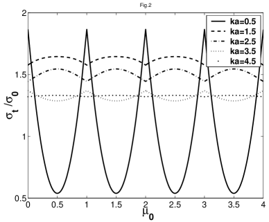
Figure 2: Periodic structures of total cross sections of a charged particle scattered by a hard sphere plus a magnetic flux along the z-axis. At quantized values of magnetic flux $\Phi=(2n+1)\Phi_{0}/2$, $n=0,1,2,\cdots$, the cross section reduces to the minimum for $ka\leq 0.5$.

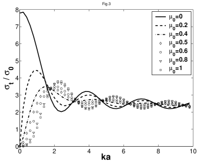
Figure 3: Total cross sections for identical bosons carrying the magnetic flux with various $\mu_{0}$. The cross section at the long wave length limit (equivalently, the sufficient short range potential), say $ka\leq 0.5$, approaches zero at the quantized magnetic flux $\Phi=(2n+1)\Phi_{0}$. On the contrary, the cross section becomes maximum and the effect of magnetic flux disappears when $\Phi=2n\Phi_{0}$. The periodic structure is $2\Phi_{0}$ as shown in Fig. 4.

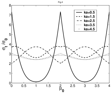
Figure 4: Periodic structures of cross sections of identical bosons carrying the magnetic flux. The cross section approaches zero when the magnetic flux is quantized at $\Phi=(2n+1)\Phi_{0}$ for $ka\leq 0.5$.

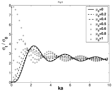
Figure 5: Total cross sections of identical fermions carrying the magnetic flux with various $\mu_{0}$. The cross section approaches zero for $ka\leq 0.5$ when the flux becomes $2n\Phi_{0}$. The magnetic flux effect disappears when the magnitude of flux is at $(2n+1)\Phi_{0}$. The global periodic structures in cross sections is $2\Phi_{0}$ as shown in Fig. 6.

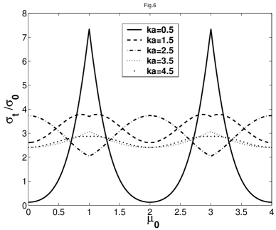
Figure 6: Periodic structures of total cross sections for identical fermions carrying the magnetic flux. The cross section approaches zero when the magnetic flux is quantized at $\Phi=2n\Phi_{0}$ for $ka\leq 0.5$.

References

- (1) Y. Aharonov and D. Bohm, Phys. Rev. 115, 485 (1959).
- (2) S. Nakajima, Y. Murayama, and A. Tonomura (Editors), Foundations of Quantum Mechanics (World Scientific, Singapore, 1996).
- (3) Z.F. Ezawa, Quantum Hall Effects (World Scientific, Singapore, 2000).
- (4) F. Wilczek, Fractional Statistics and Anyon Superconductivity (World Scientific, Singapore, 1990).
- (5) I.V. Barashenkov, and A.O. Harin, Phys. Rev. Lett. 72, 1575 (1994); Phys. Rev. D 52, 2471 (1995).
- (6) W. Hofstetter, J. König, and H. Schoeller, Phys. Rev. Lett. 87, 1568031 (2001).
- (7) D. Vion, A. Aassime, A. Cottet, P. Joyez, H. Pothier, C. Urbina, D. Esteve, and M.H. Devoret, Nature 296, 886 (2002).
- (8) A magnetic flux shielded by reflecting barriers in two dimensions were also considered by S. Olariu, and I. Iovitzu Popescu [Rev. Mod. Phys. 57, 339, 1985], but they did not consider the total cross section in terms of phase shifts.
- (9) C.A. Chatzidimitriou-Dreismann, T Abdul-Redah, R.M.F. Streffer, and J. Mayers, Phys. Rev. Lett. 79, 2839 (1997); C.A. Chatzidimitriou-Dreismann, M. Vos, C. Kleiner, and T Abdul-Redah, Phys. Rev. Lett. 91, 0574031 (2003).
- (10) R. Jackiw, Phys. Rev. Lett. 50, 555 (1983).
- (11) R. Jackiw, Phys. Rev. D 29, 2375 (1984).
- (12) A.K. Geim, S.J. Bending, and I.V. Grigorieva, Phys. Rev. Lett. 69, 2252 (1992).
- (13) S.T. Stoddart, S.J. Bending, A.K. Geim, and M. Henini, Phys. Rev. Lett. 71, 3854 (1993).
- (14) P.A.M. Dirac, Proc. Roy. Soc., Ser. A, 133, 60 (1931).
- (15) H. Kleinert, Path Integrals in Quantum Mechanics, Statistics, and Polymer Physics, 2nd edition (World Scientific, Singapore, 1995), Ch. 9.
- (16) L.S. Schulmann, J. Math. Phys. 12, 304 (1971).
- (17) T.T. Wu, and C.N. Yang, Phys. Rev. D12, 3845 (1975).
- (18) C.N. Yang, Phys. Rev. Lett. 33, 445 (1974).
- (19) D.H. Lin, J. Phys. A31, 4785 (1998); A32, 6783 (1999); A34, 2561 (2001).
- (20) D.H. Lin, J. Math. Phys. 41, 2723 (2000); W.F. Kao, P.G. Luan, and D.H. Lin, Phys. Rev. A 65, 0521081 (2002).
- (21) C.N. Yang, in Foundations of Quantum Mechanics, edited by S. Nakajima, Y. Murayama, and A. Tonomura (World Scientific, Singapore, 1996).
- (22) W. Magnus, F. Oberhettinger, R.P. Soni, Formulas and Theorems for the Special Functions of Mathematical Physics (Springer, Berlin, 1966).
- (23) V.W. Scarola, K. Park, and J.K. Jain, Nature 406, 863 (2000).
- (24) A.K. Geim, S.V. Dubonos, I.V. Grigorieva, K.S. Novoselov, F.M. Peeters, and V.A. Schweigert, Nature 407, 55 (2000).
- (25) D.H. Lin, Phys. Lett. A. 320, 207 (2003).