Bayesian Approach to Inverse Quantum Statistics: Reconstruction of Potentials in the Feynman Path Integral Representation of Quantum Theory

Abstract

The Feynman path integral representation of quantum theory is used in a non–parametric Bayesian approach to determine quantum potentials from measurements on a canonical ensemble. This representation allows to study explicitly the classical and semiclassical limits and provides a unified description in terms of functional integrals: the Feynman path integral for the statistical operator, and the integration over the space of potentials for calculating the predictive density. The latter is treated in maximum a posteriori approximation, and various approximation schemes for the former are developed and discussed. A simple numerical example shows the applicability of the method.

PACS. 02.50.Tt Inference methods - 31.15.Kb Path–integral methods - 05.30.-d Quantum statistical mechanics

1 Introduction

The solution of the quantum many–body problem requires both techniques for solving the Schrödinger equation and knowledge of the underlying forces, often to be deduced from observational data. In the field of nuclear physics, forces are extracted from scattering data and ground state properties of the two–nucleon system, since no practicable basic theory of nuclear forces exists up to date. Given a data–based phenomenological nucleon–nucleon potential, one can, in principle, construct the related potential between two colliding nuclei. However, this is a formidable task which has been attacked only for a few simple cases in an approximate way, and a direct calculation of the nucleus–nucleus potential from observational data is highly desirable for practical applications like, e.g., in nuclear astrophysics. In solid state physics the basic force is known to be the Coulomb force, however, for a straight problem like the motion of a single electron under the influence of a crystal surface, one would prefer to deduce the respective potential directly from observational data rather than going through the full many–body problem of electrons and nuclei of the crystal.

The reconstruction of such two–body forces or single–particle potentials from experimental data constitutes a typical inverse problem of quantum theory. Such problems are notoriously ill–posed in the sense of Hadamard [1] and require additional a priori information to obtain a unique, stable solution. Well–knowm examples are inverse scattering theory [2] and inverse spectral theory [3]. They describe the kind of data which are necessary, in addition to a given spectrum, to identify the potential uniquely. For example, such data can be a second spectrum for different boundary conditions, knowledge of the potential on a half–interval or the phase shifts as a function of energy. However, neither a complete spectrum nor specific values of the potential or phase shifts at all energies can be inferred by a finite number of measurements. Hence any practical algorithm for extracting two–body forces or single–particle potentials from experimental data must rely on additional a priori assumptions like symmetries, smoothness, or asymptotic behaviour. If the available data refer to a system at finite temperature $T\neq 0$, one is led to the inverse problem of quantum statistics. In such a case, non–parametric Bayesian statistics [4] is especially well suited to include both observational data and a priori information in a flexible way.

In a series of papers [5], the Bayesian approach to inverse quantum statistics has been applied to reconstruct potentials (or two–body interactions) from particle–position measurements on a canonical ensemble. A priori information was imposed through approximate symmetries (translational, periodic) or smoothness of the potential or by fixing the mean energy of the system. The likelihood model of quantum statistics (defining the probability for finding the particle at some position $x$ for a system with potential $V$ at temperature $T$) was treated in energy representation.

In the present paper we apply the Feynman path integral representation of quantum mechanics [6] to calculate the statistical operator $\rho$ and related quantities in coordinate space. This representation is of interest in the context of inverse problems in Bayesian statistics for two reasons: First, it allows to study the transition to the semiclassical and classical limits, relevant for example to atomic force microscopy [7] so far treated on the level of classical mechanics. However, scales may soon be reached where the inclusion of quantum effects will be mandatory. Second, one obtains a unified description of Bayesian statistics in terms of path integrals. These are on one side the Feynman path integrals, needed in the likelihood model, and on the other side the functional integral over the space of potential functions $V$ when calculating the predictive density as integral over the product of likelihood and posterior for all possible potentials.

Our paper is organized as follows: An introduction to Bayesian statistics is presented in section 2, showing how Bayes’ theorem about the decomposition of joint probabilities can be used for the inverse problem of quantum statistics. A general expression is given for the likelihood of a quantum system with given potential $V$ for a canonical ensemble, and the prior density is chosen as Gaussian process to implement a bias towards smoothness and/or periodicity of the potential $V$. This potential can be calculated from a non–linear differential equation which results from the maximum posterior approximation for the predictive density. Two approximation schemes for solving the inverse problem of quantum statistics in path integral representation are developed. In the first variant (sections 3 and 4), the path integral in the likelihood is treated in stationary phase approximation. The resulting stationarity equations with respect to the path are classical equations of motion for a particle in potential $-V$. These equations are to be solved simultaneously with the stationarity equations with respect to the potential, following from the maximum posterior approximation in the above classical approximation of the path integral. In the second variant (section 5), the basic stationarity equations of the maximum posterior approximation are treated in terms of the Feynman integrals. These equations which involve the logarithmic derivatives of the statistical operator and the partition function are still exact in the sense of quantum theory. Approximation schemes for the statistical operator in coordinate representation and the corresponding partition function and their derivatives are developed in sections 6 and 7. In section 6, the quadratic fluctuations for the statistical operator and the partition function around the classical paths of section 4 are determined, while section 7 deals with the respective derivatives. Three approximation schemes are studied under the general strategy that the statistical operator drops out in the logarithmic derivative. A simple numerical example is added in section 8 to show that the path integral formalism can actually be used for problems of inverse quantum statistics.

2 Bayesian Approach to Inverse Quantum Statistics

The aim of this paper is to determine the dynamical laws of quantum systems from measurements on a canonical ensemble. The method used is non-parametric Bayesian inference combined with the path integral representation of quantum theory which allows to study the transition to the classical limit. To be specific, we aim at reconstructing the potential $V$ of the system from measurements of the position coordinate $\hat{x}$ of the particle for a canonical ensemble at temperature $1\,/\,\beta$.

The general Bayesian approach, tailored to the above problem, is based on two probability densities:

1. a likelihood $p\,(x|O,\,V)$ for the probability of outcome $x$ when measuring observable $O$ for given potential $V$, not directly observable, and

2. a prior density $p\,(V)$ defined on the space ${\cal{V}}$ of possible potentials $V$.

This prior gives the probability for $V$ before data have been collected. Hence it has to comprise all a priori information available for the potential, like symmetries or smoothness. The need for a prior model, complementing the likelihood model, is characteristic for empirical learning problems which try to deduce a general law from observational data.

These ingredients, likelihood and prior, are combined in Bayes theorem to define the posterior of $V$ for given data $D$ through

$$p\,(V|D)\,=\,\frac{p\,(x_{T}|O_{T},\,V)\,p\,(V)}{p\,(x_{T}|O_{T})}\,\,.$$ (2.1)

Eq. (2.1) is a direct consequence of the decomposition of the joint probability $p\,(A,\,B)$ for two events $A,\,B$ into conditional probabilities $p\,(A|B)$ and $p\,(B|A)$, respectively. Observational data $D$ are assumed to consist of $N$ pairs,

$$D=\{(x_{i},\,O_{i})|1\,\leq\,i\,\leq\,N\}\,\,,$$ (2.2)

where $x_{T}$, $O_{T}$ denote formal vectors with components $x_{i}$, $O_{i}$. Such data are also called training data, hence the label _T. For independent data the likelihood factorizes as

$$p\,(x_{T}|O_{T},\,V)\,=\,\prod\limits_{i}\,p\,(x_{i}|O_{i},\,V)\,\,,$$ (2.3)

where a chosen observable $O_{i}$ may be measured repeatedly to give values $x_{i}$, equal or different among each other. The denominator in (2.1) can be viewed as normalization factor and can be calculated from likelihood and prior by integration over $V$,

$$p\,(x_{T}|O_{T})\,=\,\int\,DV\ p\,(x_{T}|O_{T},\,V)\,p\,(V)\,\,.$$ (2.4)

The $V$-integral in eq. (2.4) stands for an integral over parameters, if we choose a parametrized space ${\cal{V}}$ of potentials, or for a functional integral over an infinite function space.

To predict the results of future measurements on the basis of a data set $D$, one calculates according to the rules of probability theory the predictive density

$$p\,(x|O,\,D)\,=\,\int DV\ p\,(x|O,\,V)\,p\,(V|D)$$ (2.5)

which is the probability of finding value $x$ when measuring observable $O$ under the condition that data $D$ are given. Here we have assumed that the probability of $x$ is completely determined by giving potential $V$ and observable $O$, and does not depend on training data $D$, $p\,(x|O,\,V,\,D)\,=\,p\,(x|O,\,V)$, and that the probability for potential $V$ given the training data $D$ does not depend on observable $O$ selected in the future, $p\,(V|O,\,D)\,=\,p\,(V|D)$.

The integral (2.5) is high-dimensional in general and difficult to calculate in practice. Two approximations are common in Bayesian statistics: The first one is an evaluation of the integral by Monte Carlo technique. The second one, which we will pursue in this paper, is the so called maximum a posteriori approximation. Assuming the posterior to be sufficiently peaked around its maximum at potential $V^{*}$, the integral (2.5) is approximated by

$$p\,(x|O,\,D)\,\approx\,p\,(x|O,\,V^{*})$$ (2.6)

where

$$V^{*}\,=\,\text{argmax}_{V\,\in\,{\cal{V}}}\,p\,(V|D)\,=\,\text{argmax}_{V\,\in\,{\cal{V}}}\,p\,(x_{T}|O_{T},\,V)\,p\,(V)$$ (2.7)

according to eq. (2.1) with the denominator independent of $V$. Maximizing the posterior $p\,(V|D)$ with respect to $V\,\in\,{\cal{V}}$ leads to solving the stationarity equations

$$\delta_{V}\,p\,(V|D)\,=\,0\,=\,\delta_{V}\,(p\,(x_{T}|O_{T},\,V)\,p\,(V))$$ (2.8)

where $\delta_{V}$ denotes the functional derivative $\delta\,/\,\delta\,V$. Equivalent to (2.8) and technically often more convenient is the condition for the log-posterior

$$\delta_{V}\,\ln\,p\,(V|D)\,=\,0\,=\,\delta_{V}\,\ln\,p\,(x_{T}|O_{T},\,V)\,+\,\delta_{V}\,\ln\,p\,(V)$$ (2.9)

which minimizes the energy $E\,(V|D)\,=\,-\ln\,p\,(V|D)$ and will be used in the following.

A convenient choice for prior $p\,(V)$ is a Gaussian process,

$$p\,(V)\,\sim\,\exp\,\left\{-\frac{\gamma}{2}\,\langle V\,-\,V_{0}|K|V\,-\,V_{0}\rangle\right\}\,=\,\mathrm{e}^{-\frac{\gamma}{2}\,\Gamma\,[v]}$$ (2.10)

where

$$\Gamma\,[v]=\langle V-V_{0}|K|V-V_{0}\rangle=\int dx\,dx^{\prime}\,\left[v\,(x)-v_{0}\,(x)\right]\,K\,(x,\,x^{\prime})\,[v\,(x^{\prime})-v_{0}\,(x^{\prime})],$$ (2.11)

assuming a local potential $V\,(x,\,x^{\prime})\,=\,v\,(x)\,\delta\,(x\,-\,x^{\prime})$. The mean $V_{0}$ represents a reference potential or template for $V$, and the real-symmetric, positive (semi-)definite covariance operator $(\gamma\,K)^{-1}$ acts on the potential, measuring the distance between $V$ and $V_{0}$. The hyperparameter $\gamma$ is used to balance the prior against the likelihood term and is often treated in maximum a posteriori approximation or determined by cross–validation techniques. A bias towards smooth functions $v\,(x)$ can be implemented by $K\,=\,-d^{2}\,/\,dx^{2}$ choosing $v_{0}\,(x)\,\equiv\,0$. If some approximate symmetry of $v\,(x)$ is expected, like for a surface of a crystal deviating from exact periodicity due to point defects, one may implement a non-zero periodic reference potential $v_{0}\,(x)$ in eq. (2.11).

The likelihood for our problem follows from the axioms of quantum theory: The probability to find value $x$ when measuring observable $O$ for a quantum system in a state described by a statistical operator $\rho\,=\,\rho\,(V)$ is given by

$$p\,(x|O,\,V)\,=\,{\rm Tr}\,\{P_{O}\,(x)\,\rho\,(V)\}$$ (2.12)

where $P_{O}\,(x)\,=\,\Sigma_{\xi}\,|x,\,\xi\rangle\,\langle x,\,\xi|$ projects on the space spanned by the orthonormalized eigenstates $|x,\,\xi\rangle$ of operator $O$ with eigenvalue $x$, and the label $\xi$ distinguishes degenerate eigenstates with respect to $O$. If the system is not prepared in an eigenstate of observable $O$, a quantum mechanical measurement will change the state of the system, i. e., will change $\rho$. Hence to perform repeated measurements under same $\rho$ requires the restoration of $\rho$ before each measurement. For canonical ensembles at given temperature,

$$\rho=\frac{\exp(-\beta\,H)}{{\rm Tr}\exp(-\beta\,H)}$$ (2.13)

with Hamiltonian $H\,=\,T\,+\,V$ and temperature $1\,/\,\beta$, this means to wait between two consecutive observations until the system is thermalized again. Choosing the particle position operator $\hat{x}$ as observable $O$, the probability for value $x_{i}$ is

$$p\,(x_{i}|\hat{x},\,v)\,=Z^{-1}\,{\rm Tr}\{|x_{i}\rangle\,\langle x_{i}|\exp\,(-\beta\,H)\}=\frac{\langle x_{i}|\mathrm{e}^{-\beta\,H}|x_{i}\rangle}{Z}$$ (2.14)

with partition function

$$Z\,={\rm Tr}\exp\,(-\beta\,H)\,=\,\int dx\ \langle x|\exp\,(-\beta\,H)|x\rangle$$ (2.15)

where we have dropped the label $\xi$ to simplify notation. For $N$ repeated measurements of $\hat{x}$ with results $x_{i}$, $i\,=\,1,\,...\,N$, one has under the above assumptions of independent measurements

$$p\,(x_{T}|O_{T},\,V)\,=\,\prod\limits_{i}\,p\,(x_{i}|\hat{x},\,v)\,=\,\prod\limits_{i}\,\left[\langle x_{i}|\mathrm{e}^{-\beta\,H}|x_{i}\rangle\,Z^{-1}\right]\,\,.$$ (2.16)

Combining eqs. (2.10), (2.11) and (2.16) leads to the posterior

$$p\,(V|D)\,\sim\,\frac{1}{Z^{N}}\,\left(\prod\limits_{i}\,\langle x_{i}|\mathrm{e}^{-\beta\,H}|x_{i}\rangle\right)\,\exp\,\left(-\frac{\gamma}{2}\,\Gamma\,[v]\right)\,=\,\exp\,(-E\,(V|D))$$ (2.17)

with energy functional

$$E\,(V|D)\,=\,-\sum\limits_{i}\,\ln\,\langle x_{i}|\mathrm{e}^{-\beta\,H}|x_{i}\rangle\,+\,N\,\ln\,Z\,+\,\frac{\gamma}{2}\,\Gamma\,[v]\,\,,$$ (2.18)

functional $\Gamma\,[v]$ defined in eq. (2.11). The corresponding stationarity equations (2.9) in explicit form

$$-\sum\limits_{i\,=\,1}^{N}\,\frac{\frac{\delta}{\delta\,v\,(x)}\,\langle x_{i}|\mathrm{e}^{-\beta\,H}|x_{i}\rangle}{\langle x_{i}|\mathrm{e}^{-\beta\,H}|x_{i}\rangle}\,+\,\frac{N}{Z}\,\frac{\delta\,Z}{\delta\,v\,(x)}\,+\,\frac{\gamma}{2}\,\frac{\delta\,\Gamma}{\delta\,v\,(x)}\,=\,0\,\,,$$ (2.19)

with

$$\frac{1}{2}\frac{\delta\,\Gamma}{\delta\,v\,(x)}=\,K\,(v\,(x)\,-\,v_{0}\,(x))\,\,,$$ (2.20)

determine the potential $v\,(x)$.

In a series of papers [5], eqs. (2.19) have been studied successfully in energy representation for a variety of choices for prior $p\,(V)$. This requires solving the Schrödinger equation $H\,|\phi_{\alpha}\rangle\,=\,E_{\alpha}\,|\phi_{\alpha}\rangle$, $\langle\phi_{\alpha}|\phi_{\beta}\rangle\,=\,\delta_{\alpha\beta}$, which allows to calculate the functional derivatives $\delta_{v}\,E_{\alpha}$ and $\delta_{v}\,\phi_{\alpha}$ (cf. appendix) needed in eqs. (2.19). In the following sections we shall apply the path integral formulation of quantum mechanics in order to study the semiclassical as well as classical regimes.

3 Likelihood in path integral representation

The matrix elements appearing in eq. (2.16) can be written as path integrals [6]

$$\langle x_{i}|\mathrm{e}^{-\beta\,H}|x_{i}\rangle\,=\int\limits_{q\,(0)\,=\,x_{i}}^{q\,(\beta\,\hbar)\,=\,x_{i}}Dq\,(\tau)\,\exp\,\Biggl{\{}-\frac{1}{\hbar}\int\limits_{0}^{\beta\,\hbar}d\tau\left(\frac{m}{2}\,(dq\,/\,d\tau)^{2}\,+\,v\,(q)\right)\Biggr{\}}\,\,.$$ (3.1)

They are related to those of the time development operator of quantum mechanics by Wick rotation in the complex time plane. The corresponding variable transformation

$$t\,=\,-i\,\tau$$ (3.2)

replaces real time $t$ by imaginary time $\tau$ and velocity $dq\,/\,dt$ by

$$\frac{dq}{d\tau}=\,-i\frac{dq}{dt}\,,$$ (3.3)

inducing a change of sign in the kinetic energy term.

Representation (3.1) is understood as abbreviation of an infinite dimensional integral when dividing the interval $[0,\,\beta\,\hbar]$ into equidistant segments of length $\varepsilon\,=\,\beta\,\hbar\,/\,M$, coding the path $q\,(\tau)$ at discrete points $\tau_{k}\,=\,\varepsilon\,k$ by $q_{k}\,=\,q\,(\tau_{k})$ and taking the limit $M\,\to\,\infty$

$$\langle x_{i}|\mathrm{e}^{-\beta\,H}|x_{i}\rangle = \!\!\!\begin{array}[]{c}\lim\vspace*{-2mm}\\ \scriptstyle{M\to\infty}\end{array}\left(\frac{m}{2\pi\hbar\varepsilon}\right)^{\frac{M}{2}}\int\Biggl{(}\prod\limits_{k=1}^{M-1}dq_{k}\Biggr{)}$$

$$\times\,\exp\Biggl{\{}-\frac{\varepsilon}{\hbar}\sum\limits_{k=1}^{M}\!\left(\!\frac{m}{2}\left[\frac{q_{k}-q_{k-1}}{\varepsilon}\right]^{2}\!\!+v\,(q_{k})\!\right)\!\Biggr{\}}$$

$$= \int\limits_{q\,(0)\,=\,x_{i}}^{q\,(\beta\,\hbar)\,=\,x_{i}}Dq\,(\tau)\,\exp\,\left\{-\frac{1}{\hbar}\,S\,[q]\right\}\,\,,$$ (3.4)

with

$$\int\limits_{q\,(0)\,=\,x_{i}}^{q\,(\beta\,\hbar)\,=\,x_{i}}Dq\,(\tau)\,=\begin{array}[]{c}\lim\vspace*{-2mm}\\ \scriptstyle{M\to\infty}\end{array}\int\left(\prod\limits_{k\,=\,1}^{M\,-\,1}dq_{k}\right)\,\left(\frac{m}{2\,\pi\,\hbar\,\varepsilon}\right)^{\frac{M}{2}}$$ (3.5)

and Euclidean action

$$S\,[q]\,=\,\int\limits_{0}^{\beta\,\hbar}\,d\tau\,\left[\frac{m}{2}\,\dot{q}^{2}\,+\,v\,(q)\right]$$ (3.6)

where we have introduced $\dot{q}\,=\,dq/d\tau$ for short. The boundary values are fixed, $q_{0}\,=\,q_{M}\,=\,x_{i}$. The partition function $Z$ as trace in coordinate space can be written as path integral over all periodic functions $q\,(\tau)$ of fixed period $\beta\,\hbar$

$$Z={\rm Tr}(\mathrm{e}^{-\beta\,H}) = \int dx\,\langle x|\mathrm{e}^{-\beta\,H}|x\rangle\,=\int dx\int\limits_{q\,(0)\,=\,x}^{q\,(\beta\,\hbar)\,=\,x}Dq\,(\tau)\,\exp\left\{-\frac{1}{\hbar}\,S\,[q]\right\}$$ (3.7)

$$= \int\limits_{q\,(0)\,=\,q\,(\beta\,\hbar)}\!\!\!\!\!\!Dq\,(\tau)\,\exp\,\left\{-\frac{1}{\hbar}\,S\,[q]\right\}\,\,.$$

The path integral for $\langle x|\exp\,(-\beta\,H)|x\rangle$, in lowest order stationary phase approximation, is given by

$$\langle x|\exp\,(-\beta\,H)|x\rangle\,=A_{x}\,\exp\,\left(-\frac{1}{\hbar}\,S\,[q_{x}]\right)$$ (3.8)

with $q_{x}\,(\tau)$ being the solution of the classical equations of motion (4.3) with boundary conditions

$$q_{x}\,(0)\,=\,q_{x}\,(\beta\,\hbar)\,=\,x\,\,,$$ (3.9)

and factor $A_{x}$ comprising the quadratic fluctuations around the classical path $q_{x}\,(\tau)$ (see section 6, eqs. (6.7), (6.9)). The $x$-integral in $Z$, eq. (3.7), can also be treated in stationary phase approximation. The action $S\,[q]$ depends on $x$ through the boundary values of $q\,(\tau)$, and its derivative with respect to the upper (lower) boundary value of $q$ yields the corresponding momentum $\begin{array}[]{c}\scriptstyle{+\vspace*{-2mm}}\\ \scriptstyle{(-)}\end{array}p$. The stationarity condition for $S$ thus poses the additional boundary condition

$$p\,(\beta\,\hbar)\,-\,p\,(0)\,=\,0\,\,.$$ (3.10)

Hence one has to find $x_{0}$ such that the solutions of the classical equations of motion (4.3) fulfill boundary conditions for both coordinate $q\,(\tau)$ and velocity $\dot{q}\,(\tau)$,

$$q\,(0)\,=\,q\,(\beta\,\hbar)\,=\,x_{0}\quad\text{and}\quad\dot{q}\,(0)\,=\,\dot{q}\,(\beta\,\hbar)\,\,.$$ (3.11)

Then

$$Z\,=A_{0}\exp\,\left\{-\frac{1}{\hbar}\,S\,[q_{x_{0}}]\right\}$$ (3.12)

in lowest order stationary phase approximation, with $A_{0}$ the analogue of $A_{x}$, eq. (3.8).

4 Maximum posterior in stationary phase approximation

In the representation (3.1), (3.7), the posterior density reads

$$p\,(V|D)\,\sim\,\int\,\left(\prod\limits_{i\,=\,1}^{N}\,Dq_{i}\,(\tau)\right)\,\exp\,\left\{-\frac{1}{\hbar}\,\sum\limits_{i\,=\,1}^{N}\,F_{i}\,[q_{i},\,v]\right\}$$ (4.1)

with total action

$$F_{i}\,[q_{i},\,v]\,=\,S\,[q_{i},\,v]\,+\,\hbar\,\ln\,Z\,[v]\,+\,\frac{\hbar\,\gamma}{2N}\,\Gamma\,[v]\,\,,$$ (4.2)

inserting eqs. (3.4) and (3.6) into (2.17) and (2.18). Note that to each data point $x_{i}$ is assigned its own path integral.

Following the reasoning in section 2 for the $v$-integration we shall treat the integrals (3.4) in stationary phase approximation, looking for paths $q\,(\tau)$ which minimize the action $S\,[q]$ and account for the main contribution to the integrals. The corresponding stationarity equations,

$$0\,=\frac{\delta\,S}{\delta\,q_{i}}=\,-m\,\ddot{q}_{i}\,+\,\frac{d}{dq_{i}}\,v\,(q_{i})\quad\text{for}\quad i\,=\,1,\,...\,,\,N$$ (4.3)

with boundary conditions

$$q_{i}\,(0)\,=\,q_{i}\,(\beta\,\hbar)\,=\,x_{i}$$ (4.4)

are the classical equations of motion for a fictitious particle of mass $m$ in the inverted potential $-v\,(q)$ with boundary conditions determined by the data points $x_{i}$. Their solutions serve as starting points for a quantum mechanical expansion.

For each path $q_{i}\,(\tau)$ the energy

$$E_{i}\,=\,\frac{1}{2}\,m\,\dot{q}^{2}_{i}\,-\,v\,(q_{i})$$ (4.5)

is conserved. Equations (4.3), (4.4) have to be solved simultaneously with the stationarity equations (2.19), explicitly for $F=\sum_{i}F_{i}$:

$$\begin{array}[]{c}\displaystyle{0\,=\frac{\delta\,F}{\delta\,v\,(x)}=\,\sum\limits_{i\,=\,1}^{N}\,\int\limits_{0}^{\beta\,\hbar}d\tau\,\delta\,(q_{i}\,(\tau)\,-\,x)\,-\,\beta\,\hbar\,N\,\langle x|\frac{\mathrm{e}^{-\beta\,H}}{Z}|x\rangle}\\ \mbox{}\\ \displaystyle{+\,\gamma\,\hbar\,\int\,dx^{\prime}\,K\,(x,\,x^{\prime})\,(v\,(x^{\prime})\,-\,v_{0}\,(x^{\prime}))}\end{array}$$ (4.6)

for the choice (2.10) of the prior $p\,(V)$. For the derivative of $\ln\,Z$ we refer to the appendix, eq. (A.10).

The integral in the first term of (4.6) over $\delta$-distributions can be evaluated, for simple zeroes of the arguments, with the help of eq. (4.5),

$$\int\limits_{0}^{\beta\,\hbar}d\tau\,\delta\,(q_{i}\,(\tau)\,-\,x) = \sum\limits_{j_{i}\,=\,1}^{n_{i}\,(x)}\,\frac{1}{|\dot{q}_{i}\,(\tau_{j_{i}})|}\,=\,\sum\limits_{j_{i}\,=\,1}^{n_{i}\,(x)}\,\frac{1}{\sqrt{\frac{2}{m}\,(E_{i}\,+\,v\,(q_{i}\,(\tau_{j_{i}})))}}$$ (4.7)

$$= \frac{n_{i}\,(x)}{\sqrt{\frac{2}{m}\,(E_{i}\,+\,v\,(x))}},$$

$n_{i}\,(x)$ being the number of times $\tau_{j_{i}}$ with $q_{i}\,(\tau_{j_{i}})\,=\,x$, $0\,\leq\,\tau_{j_{i}}\,\leq\,\beta\,\hbar$. In the second term of (4.6), the path integral for $\langle x|\exp\,(-\beta\,H)|x\rangle$ is in lowest order stationary phase approximation given by (3.8), and analogously $Z$ by (3.12).

A compact and instructive form of condition (4.6) is obtained by multiplying with some arbitrary observable $f\,(x)\,/\,N\,\beta\,\hbar$ and integrating over $x$,

$$0 = \frac{1}{N\,\beta\,\hbar}\sum\limits_{i\,=\,1}^{N}\int\limits_{0}^{\beta\,\hbar}d\tau\,f\,(q_{i}\,(\tau))\,-\int dx\,f\,(x)\,\langle x|\frac{\mathrm{e}^{-\beta\,H}}{Z}|x\rangle$$

$$+\,\frac{\gamma}{N\,\beta}\int dx\,dx^{\prime}\,f\,(x)\,K(x,\,x^{\prime})\,[v\,(x^{\prime})\,-\,v_{0}\,(x^{\prime})]$$

$$= \frac{1}{N}\sum\limits_{i\,=\,1}^{N}\,\overline{f}_{i}\,-\,\langle f\rangle\,+\,\frac{\gamma}{N\,\beta}\,\int\,dx\,dx^{\prime}\,f\,(x)\,K(x,\,x^{\prime})\,[v\,(x^{\prime})\,-\,v_{0}\,(x^{\prime})]\,\,,$$

where $\overline{f}_{i}$ denotes the mean of $f$ with respect to (imaginary) time $\tau$ along path $q_{i}\,(\tau)$ and $\langle f\rangle$ the thermal expectation value of observable $f$. Condition (4) reminds of the ergodic theorem of statistical mechanics [8] concerning time and ensemble average, there are, however, differences in three respects:

1. the time average in (4) is over a finite interval only,

2. paths $q_{i}\,(\tau)$ refer to boundary conditions (4.4) rather than to initial conditions for $q\,(\tau)$, $\dot{q}\,(\tau)$, and

3. the prior gives a contribution to (4), non-zero in general, in contradiction to the ergodic theorem.

In the high temperature limit, $\beta\,\to\,0$, the prior term dominates condition (4), as expected, since the first two terms in (4) become $\beta$-independent. Prior knowledge $p\,(V)$ completely determines the maximum posterior solution. In contrast, the prior on $v$ becomes negligeable at low temperature, corresponding to large $\beta$-values, and the first two terms of (4) fulfill the ergodic theorem. In fact, the potential

$$v\,(x)\,=-\lim_{a\to\infty}a\,\sum\limits_{i\,=\,1}^{N}\,\delta\,(x\,-\,x_{i})$$ (4.9)

is a solution of (4.6), if the prior can be neglected. For the corresponding classical potential $-v\,(q)\,=+\lim_{a\to\infty}a\,\sum\limits_{i\,=\,1}^{N}\,\delta\,(q\,-\,x_{i})$ the equations of motion (4.3) with boundary conditions (4.4) have unstable solutions

$$q_{i}\,(\tau)\,=\,x_{i}\,\,,$$ (4.10)

and the first term in (4.6) reads

$$\sum\limits_{i\,=\,1}^{N}\int\limits_{0}^{\beta\,\hbar}d\tau\,\delta\,(q_{i}\,(\tau)-x)=\int\limits_{0}^{\beta\,\hbar}d\tau\sum\limits_{i\,=\,1}^{N}\delta\,(x_{i}-x)=\beta\,\hbar\sum\limits_{i\,=\,1}^{N}\delta\,(x_{i}-x)\,\,.$$ (4.11)

For large $\beta$-values

$$\langle x|\mathrm{e}^{-\beta\,H}|x\rangle\quad\to\quad\sum\limits_{i\,=\,1}^{N}\,\langle x|\varphi_{0i}\rangle\,\langle\varphi_{0i}|x\rangle\mathrm{e}^{-\beta E_{0}}$$ (4.12)

where the $N$-fold degenerate quantum ground state $\langle x|\varphi_{0i}\rangle$ is strongly localized by potential $v\,(x)$, eq. (4.9), around the data points $x_{i}$ such that

$$|\langle x|\varphi_{0i}\rangle|^{2}\quad\to\quad\delta\,(x\,-\,x_{i})$$ (4.13)

in proper normalization. Hence, with $Z\,=\,\sum\limits_{i\,=\,1}^{N}\,\mathrm{e}^{-\beta E_{0}}\,=\,N\mathrm{e}^{-\beta E_{0}}$, the second term in (4.6),

$$\frac{1}{Z}\,\langle x|\mathrm{e}^{-\beta\,H}|x\rangle\quad\to\quad\frac{1}{N}\,\sum\limits_{i\,=\,1}^{N}\,\delta\,(x\,-\,x_{i})\,\,,$$ (4.14)

cancels the first one, eq. (4.11).

So far we have restricted ourselves to position measurements. If given data refer to other observables, one can use closure relations to calculate the required matrix elements in those observables while retaining the above path integral formalism. A typical example would be particle momenta rather than positions. In this case, Fourier transformation leads to

$$\langle\tilde{p}|\mathrm{e}^{-\beta\,H}|\tilde{p}\rangle = \int dx\,dx^{\prime}\,\langle\tilde{p}|x^{\prime}\rangle\,\langle x^{\prime}|\mathrm{e}^{-\beta\,H}|x\rangle\,\langle x|\tilde{p}\rangle$$ (4.15)

$$\sim \int dx\,dx^{\prime}\int\limits_{q\,(0)\,=\,x}^{q\,(\beta\,\hbar)\,=\,x^{\prime}}Dq\,(\tau)\,\exp\,\left\{-\frac{1}{\hbar}\,\left(S\,[q]\,+\,i\,\tilde{p}\,(x^{\prime}\,-\,x)\right)\right\}$$

$$= \int Dq\,(\tau)\,\exp\,\left\{-\frac{1}{\hbar}\,\Big{(}S\,[q]\,+\,i\,\tilde{p}\,\big{(}q\,(\beta\,\hbar)\,-\,q\,(0)\big{)}\Big{)}\right\}$$

where the integration is over all path $q\,(\tau)$ of the interval $[0,\,\beta\,\hbar]$. Integral (4.15) may then be calculated in saddle point approximation. Before presenting a numerical case study to show that the above formalism is feasible in practice, we will study an alternative approach to the path integral representation.

5 Maximum posterior stationarity equations in path integral representation

In this section we start from the general stationarity equations (2.19) for the posterior, restricting ourselves to the case of position measurements for the sake of definiteness. The terms in (2.19) which result from the likelihood can all be expressed in terms of the basic path integral (3.1). As the matrix elements $\langle x_{i}|\mathrm{e}^{-\beta\,H}|x_{i}\rangle$ and partition function $Z\,=\,\int dx\,\langle x|\mathrm{e}^{-\beta\,H}|x\rangle$ need no further comment, we will directly proceed to evaluate their derivatives with respect to $v$.

According to (3.7), the functional derivative of $Z$ leads to

$$\frac{\delta\,Z}{\delta\,v\,(x^{\prime})} = -\frac{1}{\hbar}\,\int\limits_{q\,(0)\,=\,q\,(\beta\,\hbar)}\!\!\!\!Dq\,(\tau)\,\exp\,\left\{-\frac{1}{\hbar}\,S\,[q]\right\}\int\limits_{0}^{\beta\,\hbar}d\tau^{\prime}\,\delta\,(q\,(\tau^{\prime})\,-\,x^{\prime})$$

$$= -\frac{1}{\hbar}\int\limits_{0}^{\beta\,\hbar}d\tau^{\prime}\int\limits_{q\,(0)\,=\,q\,(\beta\,\hbar)}\!\!\!\!Dq\,(\tau)\,\exp\left\{-\frac{1}{\hbar}\,S\,[q]\right\}\delta\,(q\,(\tau^{\prime})\,-\,x^{\prime})\,,$$

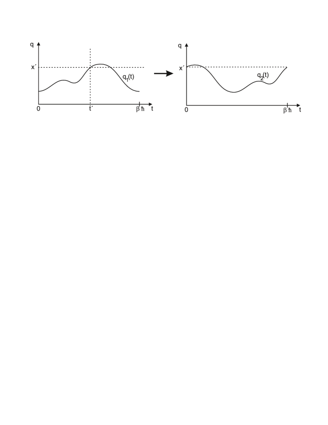
Figure 1: Equivalent paths $q_{1}\,(\tau)$ and $q_{2}\,(\tau)$ in the interval $[0,\,\hbar\,\beta]$, explaining eq. (5.2). (In the figure $\tau$ is denoted $t$.)

interchanging the order of integration in the second step. To evaluate the above path integral we observe that action $S\,[q]$ and measure $Dq\,(\tau)$ are invariant under cyclic shift of each path $q\,(\tau)$ around some arbitrary value $\tau^{\prime}$. This is displayed in Fig. 1 where the two paths $q_{1}\,(\tau)$, $q_{2}\,(\tau)$ cover the same set of values in the interval $[0,\,\beta\,\hbar]$ and thus generate the same value for the integral $\int d\tau\,v\,(q\,(\tau))$. The same reasoning holds for the derivatives $\dot{q}_{1}$, $\dot{q}_{2}$, hence $\int d\tau\,(\dot{q}\,(\tau))^{2}$ also has the same value for the two paths. Therefore the path integral in (LABEL:4.1), running over all periodic paths which go through point $x^{\prime}$ at time $\tau^{\prime}$, can be expressed as the path integral over all paths which start and end at $x^{\prime}$:

$$\int\limits_{q\,(0)\,=\,q\,(\beta\,\hbar)}\!\!\!\!Dq\,(\tau)\,\exp\,\left\{-\frac{1}{\hbar}\,S\,[q]\right\}\delta\,(q\,(\tau^{\prime})\,-\,x^{\prime})$$

$$=\int\limits_{q\,(0)\,=\,x^{\prime}}^{q\,(\beta\,\hbar)\,=\,x^{\prime}}\!\!\!\!Dq\,(\tau)\,\exp\,\left\{-\frac{1}{\hbar}\,S\,[q]\right\}$$

$$=\langle x^{\prime}|\mathrm{e}^{-\beta\,H}|x^{\prime}\rangle\,\,,$$ (5.2)

using eq. (3.1). Note that (5.2) holds independent of the choice of $\tau^{\prime}$. The remaining integral in (LABEL:4.1) is then trivial, $\int\limits_{0}^{\beta\,\hbar}d\tau^{\prime}\,=\,\beta\,\hbar$, confirming the expected result

$$\frac{\delta\,Z}{\delta\,v\,(x^{\prime})}=\,\frac{\delta}{\delta\,v\,(x^{\prime})}\int dx\,\langle x|\mathrm{e}^{-\beta\,H}|x\rangle\,=\,-\beta\,\langle x^{\prime}|\mathrm{e}^{-\beta\,H}|x^{\prime}\rangle\,\,.$$ (5.3)

In the functional derivative of matrix elements $\langle x_{i}|\mathrm{e}^{-\beta\,H}|x_{i}\rangle$ with respect to $v$,

$$\frac{\delta}{\delta\,v\,(x^{\prime})}\,\langle x_{i}|\mathrm{e}^{-\beta\,H}|x_{i}\rangle = \!\!\!\!-\frac{1}{\hbar}\int\limits_{0}^{\beta\,\hbar}d\tau^{\prime}\!\!\!\!\int\limits_{q\,(0)\,=\,x_{i}}^{q\,(\beta\,\hbar)\,=\,x_{i}}\!\!\!\!\!\!Dq\,(\tau)\,\exp\,\left\{-\frac{1}{\hbar}\,S\,[q]\right\}\,\delta\,(q\,(\tau^{\prime})\,-\,x^{\prime})$$ (5.4)

$$= \!\!\!\!-\frac{1}{\hbar}\int\limits_{0}^{\beta\,\hbar}d\tau^{\prime}\!\!\!\!\int\limits_{\begin{array}[]{c}\scriptstyle{q\,(0)\,=\,x_{i}}\\ \scriptstyle{q\,(\tau^{\prime})\,=\,x^{\prime}}\end{array}}^{q\,(\beta\,\hbar)\,=\,x_{i}}\!\!\!\!Dq\,(\tau)\,\exp\,\left\{-\frac{1}{\hbar}\,S\,[q]\right\}\,\,,$$

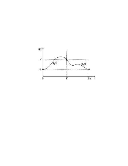
Figure 2: Splitting path $q\,(\tau)$ into parts $q_{1}\,(\tau)$ and $q_{2}\,(\tau)$, explaining the transition from eq. (5.4) to (5.5). (In the figure $\tau$, $\tau^{\prime}$ are denoted $t$, $t^{\prime}$, respectively.)

the path integral is split into two separate integrals according to Fig. 2. Taking into account the boundary conditions for the paths $q_{1}\,(\tau)$, $q_{2}\,(\tau)$ on the $\tau$-axis, one obtains, under the $\tau^{\prime}$-integral, a product of non-diagonal matrix elements of the statistical operator at different temperatures,

$$\begin{array}[]{c}\displaystyle{\frac{\delta\,\langle x_{i}|\mathrm{e}^{-\beta\,H}|x_{i}\rangle}{\delta\,v\,(x^{\prime})}=}\\ \mbox{}\\ \displaystyle{-\frac{1}{\hbar}\!\!\!\int\limits_{0}^{\beta\,\hbar}d\tau^{\prime}\int\limits_{q_{2}\,(\tau^{\prime})\,=\,x^{\prime}}^{q_{2}\,(\beta\,\hbar)\,=\,x_{i}}\!\!\!Dq_{2}\,(\tau)\,\exp\left\{-\frac{1}{\hbar}S_{2}\,[q_{2}]\right\}\!\!\int\limits_{q_{1}\,(0)\,=\,x_{i}}^{q_{1}\,(\tau^{\prime})\,=\,x^{\prime}}\!\!\!Dq_{1}\,(\tau)\,\exp\left\{-\frac{1}{\hbar}\,S_{1}\,[q_{1}]\right\}}\\ \mbox{}\\ \displaystyle{=\,-\frac{1}{\hbar}\int\limits_{0}^{\beta\,\hbar}d\tau^{\prime}\,\langle x_{i}|\exp\,\left\{-\left(\beta\,-\,\frac{\tau^{\prime}}{\hbar}\right)\,H\right\}|x^{\prime}\rangle\,\langle x^{\prime}|\exp\,\left\{-\frac{\tau^{\prime}}{\hbar}\,H\right\}|x_{i}\rangle}\\ \mbox{}\\ \displaystyle{=\,-\int\limits_{0}^{\beta}\,d\beta^{\prime}\,\langle x_{i}|\exp\,\{-(\beta\,-\,\beta^{\prime})\,H\}|x^{\prime}\rangle\,\langle x^{\prime}|\exp\,\{-\beta^{\prime}\,H\}|x_{i}\rangle}\end{array}$$ (5.5)

where the full action $S\,[q]$ is split into parts,

$$\begin{array}[]{c}\displaystyle{S_{1}\,[q_{1}]\,=\int\limits_{0}^{\tau^{\prime}}d\tau\,\left(\frac{m}{2}\,\dot{q}_{1}^{2}\,+\,v_{1}\,(q_{1})\right)}\\ \mbox{}\\ \text{and}\\ \mbox{}\\ \displaystyle{S_{2}\,[q_{2}]\,=\int\limits_{\tau^{\prime}}^{\beta\,\hbar}d\tau\,\left(\frac{m}{2}\,\dot{q}^{2}_{2}\,+\,v_{2}\,(q_{2})\right)\,\,.}\end{array}$$ (5.6)

The results (5.3), (5.5) and (5.6) obtained from the basic path integral (3.1) are still exact, in particular they are strictly equivalent to the respective expressions in energy representation (see appendix). With the above formulae, stationarity equations (2.19) read

$$\begin{array}[]{c}\displaystyle{\sum\limits_{i\,=\,1}^{N}\int\limits_{0}^{\beta}\,d\beta^{\prime}\,\frac{\langle x_{i}|\exp\,(-(\beta\,-\,\beta^{\prime})\,H)|x^{\prime}\rangle\,\langle x^{\prime}|\exp\,(-\beta^{\prime}\,H)|x_{i}\rangle}{\langle x_{i}|\exp\,(-\beta\,H)|x_{i}\rangle}\,-\,N\,\beta\,\langle x^{\prime}|\frac{\mathrm{e}^{-\beta\,H}}{Z}|x^{\prime}\rangle}\\ \mbox{}\\ \displaystyle{=\,-\frac{\gamma}{2}\frac{\delta\,\Gamma}{\delta\,v\,(x^{\prime})}=\,-\gamma\,K\,(v\,(x^{\prime})\,-\,v_{0}\,(x^{\prime}))}\end{array}$$ (5.7)

for the prior of eqs. (2.10), (2.11).

In the following sections we shall study approximation schemes for the above derivatives (5.3) and (5.5). It will be shown under what assumptions the exact (quantum mechanical) result (5.7) approaches the approximate (semiclassical) form (4.6), and how to find corrections to (4.6) taking into account quantum fluctuations around the classical paths $q_{i}\,(\tau)$ of equations (4.3), (4.4).

6 Quadratic fluctuations

Matrix elements

$$\langle x|\mathrm{e}^{-\beta\,H}|x\rangle\,=\int\limits_{q\,(0)\,=\,x}^{q\,(\beta\,\hbar)\,=\,x}Dq\,(\tau)\,\exp\,\left\{-\frac{1}{\hbar}\,S\,[q]\right\}$$ (6.1)

can be handled by standard techniques, starting from the stationarity equations (4.3), (4.4). They read, dropping the label ${i}$ and using $v^{\prime}\,=\,dv/\,dq_{x}$ for simplicity of notation,

$$0\,=\frac{\delta\,S}{\delta\,q}=\,-m\,\ddot{q}\,+\,v^{\prime}\,(q)\quad\text{with}\quad q\,(0)\,=\,q\,(\beta\,\hbar)\,=\,x\,\,.$$ (6.2)

The stationary solutions $q_{x}\,(\tau)$ of (6.2) yield the main contribution to the path integral (6.1); fluctuations around these solutions $q_{x}\,(\tau)$ can be taken care of by a variable transformation

$$q\,(\tau)\,=\,q_{x}\,(\tau)\,+\,r\,(\tau)\quad\text{with}\quad r\,(0)\,=\,r\,(\beta\,\hbar)\,=\,0\,\,.$$ (6.3)

Assuming that only small deviations of $q\,(\tau)$ from $q_{x}\,(\tau)$ are important for the integral (6.1), we approximate

$$v\,(q)\,=\,v\,(q_{x})\,+\,(q\,-\,q_{x})\,v^{\prime}\,(q_{x})\,+\,\frac{1}{2}\,(q\,-\,q_{x})^{2}\,v^{{}^{\prime\prime}}\,(q_{x})$$ (6.4)

and find for the action

$$S\,[q] = \int\limits_{0}^{\beta\,\hbar}\,d\tau\,\left(\frac{m}{2}\,\dot{q}^{2}_{x}\,+\,\frac{m}{2}\,\dot{r}^{2}\,+\,m\,\dot{q}_{x}\,\dot{r}\,+\,v\,(q_{x}\,+\,r)\right)$$ (6.5)

$$= \int\limits_{0}^{\beta\,\hbar}d\tau\,\left(\frac{m}{2}\,\dot{q}^{2}_{x}\,+\,v\,(q_{x})\right)\,+\int\limits_{0}^{\beta\,\hbar}d\tau\,\left(\frac{m}{2}\,\dot{r}^{2}\,+\,\frac{1}{2}\,v^{{}^{\prime\prime}}\,(q_{x})\,r^{2}\right)$$

$$+\,\int\limits_{0}^{\beta\,\hbar}\,d\tau\,\Big{(}m\,\dot{q}_{x}\,\dot{r}\,+\,v^{\prime}\,(q_{x})\,r\Big{)}$$

where the last term vanishes by virtue of (6.2), (6.3) and partial integration

$$\int\limits_{0}^{\beta\,\hbar}d\tau\,[m\,\dot{q}_{x}\,\dot{r}\,+\,v^{\prime}\,(q_{x})\,r]\,=\,\left[m\,\dot{q}_{x}\,r\right]^{\beta\,\hbar}_{0}\,=\,0\,\,.$$ (6.6)

For the additive action (6.5), (6.6) the matrix element (6.1) factorizes

$$\begin{array}[]{c}\displaystyle{\langle x|\mathrm{e}^{-\beta\,H}|x\rangle=A_{x}\exp\left\{-\frac{1}{\hbar}\,S\,[q_{x}]\right\}}\\ \displaystyle{=\exp\,\left\{-\frac{1}{\hbar}\,S\,[q_{x}]\right\}\int\limits_{r\,(0)\,=\,0}^{r\,(\beta\,\hbar)\,=\,0}Dr\,(\tau)}\\ \displaystyle{\times\,\,\exp\,\left\{-\frac{1}{\hbar}\int\limits_{0}^{\beta\,\hbar}\!d\tau\,\left(\frac{m}{2}\,\dot{r}^{2}+\frac{1}{2}\,v^{{}^{\prime\prime}}\,(q_{x})\,r^{2}\right)\right\}}\\ \mbox{}\\ \displaystyle{=\exp\,\left\{-\frac{1}{\hbar}\,S\,[q_{x}]\right\}\int\limits_{r\,(0)\,=\,0}^{r\,(\beta\,\hbar)\,=\,0}Dr\,(\tau)}\\ \displaystyle{\times\,\,\exp\,\left\{-\frac{1}{2\,\hbar}\int\limits_{0}^{\beta\,\hbar}\!\!d\tau\,d\tau^{\prime}\,r\,(\tau^{\prime})\left(\frac{\delta^{2}\,S\,[q]}{\delta\,q\,(\tau^{\prime})\,\delta\,q\,(\tau)}\Bigg{|}_{q\,=\,q_{x}}\right)\,r\,(\tau)\right\}}\end{array}$$ (6.7)

with Hesse-matrix

$$\frac{\delta^{2}\,S\,[q]}{\delta\,q\,(\tau^{\prime})\,\delta\,q\,(\tau)}\Biggr{|}_{q\,=\,q_{x}}\,=\,\delta\,(\tau\,-\,\tau^{\prime})\,\left(-m\,\frac{\partial^{2}}{\partial\,\tau^{2}}\,+\,v^{{}^{\prime\prime}}\,(q_{x}\,(\tau))\right)\,\,,$$ (6.8)

in approximation (6.4). For the integral in (6.7) to be well-defined, the Hesse-matrix (6.8) has to be positive-definite. Under the expansion (6.4) this holds if $v^{{}^{\prime\prime}}\,(x)\,>\,0$ for all $x$.

The remaining path integral (6.7) can be evaluated by the ‘shifting method’. We shall simply recall the result, known in the literature as van Vleck–formula [9]:

$$\langle x|\mathrm{e}^{-\beta\,H}|x\rangle = A_{x}\exp\left\{-\frac{1}{\hbar}\,S\,[q_{x}]\right\}$$ (6.9)

$$= \left(\frac{2\,\pi\,\hbar}{m}\,\kappa_{x}\,(\beta\,\hbar)\,\kappa_{x}\,(0)\int\limits_{0}^{\beta\,\hbar}\frac{d\tau}{\kappa^{2}_{x}\,(\tau)}\right)^{-\frac{1}{2}}\exp\,\left\{-\frac{1}{\hbar}\,S\,[q_{x}]\right\}$$

$$= \left(-\frac{1}{2\,\pi\,\hbar}\,\frac{\partial^{2}\,S\,[q_{x}]}{\partial\,x^{2}}\right)^{\frac{1}{2}}\,\exp\,\left\{-\frac{1}{\hbar}\,S\,[q_{x}]\right\}$$

with $\kappa_{x}\,(\tau)$ a solution of

$$v^{{}^{\prime\prime}}\,(q_{x}\,(\tau))\,=\,m\,\frac{\ddot{\kappa}_{x}\,(\tau)}{\kappa_{x}\,(\tau)}\,\,.$$ (6.10)

If $\dot{q}_{x}$ does not vanish on the path $q_{x}\,(\tau)$, one can choose

$$\kappa_{x}\,(\tau)\,=\,\dot{q}_{x}\,(\tau)\,\,,$$ (6.11)

as is easily seen by differentiating (6.2) with respect to $\tau$. Otherwise we look for a linear combination of the two linearly independent solutions $\kappa^{(1)}_{x}\,(\tau)\,=\,\dot{q}_{x}\,(\tau)$ and

$$\kappa^{(2)}_{x}\,(\tau)\,=\,\dot{q}_{x}\,(\tau)\int\limits^{\tau}\frac{d\tau^{\prime}}{(\dot{q}_{x}\,(\tau^{\prime}))^{2}}\,\,.$$ (6.12)

The latter solution follows from the fact that the Wronski determinant of eq. (6.2) is constant.

For the partition function $Z$ we use the result (6.7), (6.9) for the matrix element of the statistical operator

$$Z=\int dx^{\prime}\,A_{x^{\prime}}\exp\,\left\{-\frac{1}{\hbar}\,S\,[q_{x^{\prime}}]\right\},$$ (6.13)

and the $x^{\prime}$–integration is done numerically. Combining (6.7) and (6.13) results in the normalized matrix element of the statistical operator in coordinate representation

$$\langle x|\mathrm{e}^{-\beta\,H}|x\rangle\,/\,Z\,=\,\frac{A_{x}\exp\,\left\{-\frac{1}{\hbar}\,S\,[q_{x}]\right\}}{\int dx^{\prime}\,A_{x^{\prime}}\exp\,\left\{-\frac{1}{\hbar}\,S\,[q_{x^{\prime}}]\right\}}.$$ (6.14)

For large masses $m$, formula (6.7) reproduces the result of classical statistical mechanics. In this case, the equations of motion (6.2) simplify,

$$\ddot{q}_{x}\,=\,\frac{1}{m}\,v^{\prime}\,(q_{x})\,\to\,0\quad\text{for}\quad m\,\to\,\infty\,\,,$$ (6.15)

and are solved by the static paths

$$q_{x}\,(\tau)\,=\,x$$ (6.16)

for the boundary conditions of (6.2). Then from (6.7)

$$\langle x|\mathrm{e}^{-\beta\,H}|x\rangle\to\exp\,(-\beta\,v\,(x))\!\!\!\int\limits_{r\,(0)\,=\,0}^{r\,(\beta\,\hbar)\,=\,0}\!\!\!Dr\,(\tau)\,\exp\left\{-\frac{1}{\hbar}\int\limits^{\beta\,\hbar}_{0}\!\!d\tau\!\left(\frac{m}{2}\dot{r}^{2}+\frac{1}{2}v^{{}^{\prime\prime}}\,(x)\,r^{2}\!\right)\!\right\}$$ (6.17)

In the limit of large masses, $v^{{}^{\prime\prime}}\,(x)\,/\,m\,\to\,0$, the remaining integral in (6.17) becomes independent of $x$ so that the classical result is obtained:

$$\langle x|\mathrm{e}^{-\beta\,H}|x\rangle\,/\,Z\,=\,\frac{\exp\,(-\beta\,v\,(x))}{\int dx^{\prime}\,\exp\,(-\beta\,v\,(x^{\prime}))}\,\,.$$ (6.18)

7 Matrix elements of the derivative of the statistical operator with respect to the potential

Three variants of approximations for the derivative

$$\frac{\delta}{\delta\,v\,(x^{\prime})}\,\langle x_{i}|\mathrm{e}^{-\beta\,H}|x_{i}\rangle\,=\,-\frac{1}{\hbar}\!\int\limits_{0}^{\beta\,\hbar}d\tau^{\prime}\int\limits_{q\,(0)\,=\,x_{i}}^{q\,(\beta\,\hbar)\,=\,x_{i}}\!\!\!Dq\,(\tau)\,\exp\,\left\{\!-\frac{1}{\hbar}\,S\,[q]\right\}\,\delta\,(q\,(\tau^{\prime})\,-\,x^{\prime})$$ (7.1)

are presented. The general strategy is to find approximations such that in the logarithmic derivative of the statistical operator, needed in (2.19), the statistical operator drops out.

In the first approach, we observe that the main contribution to the path integral stems from the stationary path $q_{x_{i}}\,(\tau)$, solution of eqs. (4.3), (4.4). Hence the distribution $\delta\,(q\,(\tau^{\prime})\,-\,x^{\prime})$ under the path integral in (7.1) may be replaced by $\delta\,(q_{x_{i}}\,(\tau^{\prime})\,-\,x^{\prime})$, referring to the stationary path, in front of the path integral. In this approximation,

$$\frac{\delta}{\delta\,v\,(x^{\prime})}\langle x_{i}|\mathrm{e}^{-\beta\,H}|x_{i}\rangle=-\frac{1}{\hbar}\left\{\!\int\limits_{0}^{\beta\,\hbar}\!d\tau^{\prime}\delta(q_{x_{i}}(\tau^{\prime})-x^{\prime})\!\right\}\!\!\int\limits_{q\,(0)\,=\,x_{i}}^{q\,(\beta\,\hbar)\,=\,x_{i}}\!\!\!\!\!\!\!\!\!Dq\,(\tau)\exp\left\{-\frac{1}{\hbar}S\,[q]\right\},$$ (7.2)

the first term in the stationarity equation (2.19) takes the form

$$\frac{\frac{\delta}{\delta\,v\,(x^{\prime})}\,\langle x_{i}|\mathrm{e}^{-\beta\,H}|x_{i}\rangle}{\langle x_{i}|\mathrm{e}^{-\beta\,H}|x_{i}\rangle}\,=\,-\frac{1}{\hbar}\int\limits_{0}^{\beta\,\hbar}d\tau^{\prime}\,\delta\,(q_{x_{i}}\,(\tau^{\prime})\,-\,x^{\prime})$$ (7.3)

in agreement with the first term in (4.6). One may improve on the result (7.3) by applying approximation (7.2) after the classical action $S\,[q_{x_{i}}]$ has been factored out with the help of the variable transformation (6.3). Then, using (6.7),

$$\begin{array}[]{c}\displaystyle{\frac{\delta}{\delta\,v\,(x^{\prime})}\,\langle x_{i}|\mathrm{e}^{-\beta\,H}|x_{i}\rangle\,=\,-\frac{\exp\,\left\{-\frac{1}{\hbar}\,S\,[q_{x_{i}}]\right\}}{\hbar}\int\limits^{\beta\,\hbar}_{0}d\tau^{\prime}\int\limits_{r\,(0)\,=\,0}^{r\,(\beta\,\hbar)\,=\,0}Dr\,(\tau)}\\ \mbox{}\\ \displaystyle{\times\,\,\delta\,(q_{x_{i}}\,(\tau^{\prime})\,+\,r\,(\tau^{\prime})\,-\,x^{\prime})\,\exp\,\left\{-\frac{1}{\hbar}\,S\,[r]\right\}}\\ \mbox{}\\ \displaystyle{\approx-\frac{\exp\left\{-\frac{1}{\hbar}\,S\,[q_{x_{i}}]\right\}}{\hbar}\!\int\limits_{0}^{\beta\,\hbar}\!\!d\tau^{\prime}\,\delta\,(q_{x_{i}}\,(\tau^{\prime})+r_{x_{i}}\,(\tau^{\prime})-x^{\prime})\!\!\!\!\!\!\int\limits_{r\,(0)\,=\,0}^{r\,(\beta\,\hbar)\,=\,0}\!\!\!\!\!Dr\,(\tau)\exp\left\{-\frac{1}{\hbar}S\,[r]\!\right\}}\end{array}$$ (7.4)

where $r_{x_{i}}\,(\tau)$ is the solution of

$$m\,\ddot{r}_{x_{i}}\,=\,v^{{}^{\prime\prime}}\,(q_{x_{i}}\,(\tau))\,r_{x_{i}}\quad\text{for}\quad r_{x_{i}}\,(0)\,=\,0\,=\,r_{x_{i}}\,(\beta\,\hbar)\,\,,$$ (7.5)

and

$$S\,[r]\,=\int\limits_{0}^{\beta\,\hbar}d\tau\,\left(\frac{1}{2}\,m\,\dot{r}^{2}\,+\,\frac{1}{2}\,\,v^{{}^{\prime\prime}}\,(q_{x_{i}}\,(\tau))\,r^{2}\right)\,\,.$$ (7.6)

With (6.7),

$$\langle x_{i}|\mathrm{e}^{-\beta\,H}|x_{i}\rangle\,=\,\exp\,\left\{-\frac{1}{\hbar}\,S\,[q_{x_{i}}]\right\}\int\limits_{r\,(0)\,=\,0}^{r\,(\beta\,\hbar)\,=\,0}\!\!\!Dr\,(\tau)\,\exp\,\left\{-\frac{1}{\hbar}\,S\,[r]\right\}\,\,,$$ (7.7)

one finally has

$$\frac{\frac{\delta}{\delta\,v\,(x^{\prime})}\langle x_{i}|\mathrm{e}^{-\beta\,H}|x_{i}\rangle}{\langle x_{i}|\mathrm{e}^{-\beta\,H}|x_{i}\rangle}\,=\,-\frac{1}{\hbar}\int\limits_{0}^{\beta\,\hbar}d\tau^{\prime}\,\delta\,\Big{(}q_{x_{i}}\,(\tau^{\prime})\,+\,r_{x_{i}}\,(\tau^{\prime})\,-\,x^{\prime}\Big{)}\,\,.$$ (7.8)

A second possibility to evaluate the derivative of the statistical operator consists of inserting the spectral representation of the $\delta$-distribution into (7.1). With $q\,(\tau)\,=\,q_{x_{i}}\,(\tau)\,+\,r\,(\tau)$ one obtains, in approximation (6.4), for

$$\begin{array}[]{c}\displaystyle{\frac{\delta}{\delta\,v\,(x^{\prime})}\,\langle x_{i}|\mathrm{e}^{-\beta\,H}|x_{i}\rangle=\,-\frac{1}{\hbar}\,\exp\,\left\{-\frac{1}{\hbar}\,S\,[q_{x_{i}}]\right\}\!\!\int\limits_{0}^{\beta\,\hbar}\!\!d\tau^{\prime}\!\!\!\int\!\frac{d\lambda}{2\,\pi}\exp\left\{i\,\lambda\,(q_{x_{i}}\,(\tau^{\prime})-x^{\prime})\right\}}\\ \mbox{}\\ \displaystyle{\times\int\limits_{r\,(0)\,=\,0}^{r\,(\beta\,\hbar)\,=\,0}\!\!\!Dr\,(\tau)\exp\left\{-\frac{1}{\hbar}\!\!\int\limits_{0}^{\beta\,\hbar}\!\!d\tau\left(\frac{m}{2}\,\dot{r}^{2}\,+\,\frac{1}{2}\,v^{{}^{\prime\prime}}\,(q_{x_{i}})\,r^{2}-i\,\lambda\,\hbar\,\delta(\tau-\tau^{\prime})\,r(\tau)\right)\right\}}\end{array}$$ (7.9)

a path integral where a $\delta$-like potential appears in the action in addition to the harmonic potential with time dependent frequency. Looking for saddle points of the path integral leads to the inhomogeneous equation of motion

$$-m\,\ddot{r}_{x_{i}\,\tau^{\prime}\,\lambda}\,(\tau)\,+\,v^{\prime\prime}(q_{x_{i}}(\tau))\,r_{x_{i}\,\tau^{\prime}\,\lambda}\,=\,i\,\lambda\,\hbar\,\delta\,(\tau\,-\,\tau^{\prime})$$ (7.10)

with boundary conditions

$$r_{x_{i}\,\tau^{\prime}\,\lambda}\,(0)\,=\,r_{x_{i}\,\tau^{\prime}\,\lambda}\,(\beta\,\hbar)\,=\,0\,\,.$$ (7.11)

Note that the solutions of (7.10), (7.11) are both $\lambda$- and $\tau^{\prime}$-dependent. The path $r_{x_{i}\,\tau^{\prime}\,\lambda}$ is intimately related to the Green function $R_{x_{i}}\,(\tau,\,\tau^{\prime})$ of the operator $-m\,\frac{d^{2}}{d\tau^{2}}\,+\,v^{{}^{\prime\prime}}\,(q_{x_{i}}\,(\tau))$ with the above boundary conditions,

$$-m\,\ddot{R}_{x_{i}}\,(\tau,\,\tau^{\prime})\,+\,v^{{}^{\prime\prime}}\,(q_{x_{i}}\,(\tau))\,R_{x_{i}}\,(\tau,\,\tau^{\prime})\,=\,\delta\,(\tau\,-\,\tau^{\prime})$$ (7.12)

with

$$R_{x_{i}}\,(0,\,\tau^{\prime})\,=\,R_{x_{i}}\,(\beta\,\hbar,\,\tau^{\prime})\,=\,0\,\,,$$ (7.12’)

namely

$$r_{x_{i}\,\tau^{\prime}\,\lambda}\,(\tau)\,=\,i\,\hbar\,\lambda\,R_{x_{i}}\,(\tau,\,\tau^{\prime})\,\,.$$ (7.13)

Furthermore, multiplying (7.10) by $r_{x_{i}\,\tau^{\prime}\,\lambda}\,(\tau)$ and integrating over $\tau$, one obtains for the quadratic part of the stationary action of (7.9)

$$-\frac{1}{\hbar}\int\limits_{0}^{\beta\,\hbar}\!\!d\tau\left(\frac{1}{2}\,m\,\dot{r}^{2}_{x_{i}\,\tau^{\prime}\,\lambda}+\frac{1}{2}\,v^{{}^{\prime\prime}}\,(q_{x_{i}}\,(\tau))\,r_{x_{i}\,\tau^{\prime}\lambda}^{2}\right)\! = -\frac{i\,\lambda}{2}\,r_{x_{i}\tau^{\prime}\lambda}(\tau^{\prime})$$ (7.14)

$$= \frac{\lambda^{2}\hbar}{2}\,R_{x_{i}}\,(\tau^{\prime},\,\tau^{\prime})$$

Here use has been made of a partial integration, $-\int d\tau\,\dot{r}^{2}\,=\int d\tau\,r\,\ddot{r}$, and of eqs. (7.10) and (7.11). After further variable transformation,

$$r\,(\tau)\,=\,r_{x_{i}\,\tau^{\prime}\,\lambda}\,(\tau)\,+\,l\,(\tau)\,\,,$$ (7.15)

one finds that in the action of eq. (7.9)

$$\begin{array}[]{c}\displaystyle{\int\limits_{0}^{\beta\,\hbar}\!\!d\tau\,\Bigl{(}m\,\dot{r}_{x_{i}\,\tau^{\prime}\,\lambda}\,(\tau)\,\dot{l}\,(\tau)\,+\,v^{{}^{\prime\prime}}\,(q_{x_{i}}\,(\tau))\,r_{x_{i}\,\tau^{\prime}\,\lambda}\,(\tau)\,l\,(\tau)\,-\,i\,\hbar\lambda\,l\,(\tau)\,\delta\,(\tau-\tau^{\prime})\Bigr{)}}\\ \mbox{}\\ =\,[m\,\dot{r}_{x_{i}\,\tau^{\prime}\,\lambda}\,(\tau)\,l\,(\tau)]^{\beta\,\hbar}_{0}\,=\,0\end{array}$$ (7.16)

so that (7.9) reads, under approximation (7.2),

$$\begin{array}[]{c}\displaystyle{\frac{\delta\,\langle x_{i}|\mathrm{e}^{-\beta\,H}|x_{i}\rangle}{\delta\,v\,(x^{\prime})}=-\frac{1}{\hbar}\,\exp\,\left\{-\frac{1}{\hbar}\,S\,[q_{x_{i}}]\right\}\!\!\int\limits_{0}^{\beta\,\hbar}\!\!\!d\tau^{\prime}\,\Biggl{[}\int\frac{d\lambda}{2\,\pi}\exp\Biggl{\{}i\,\lambda\,(q_{x_{i}}\,(\tau^{\prime})\,+}\\ \mbox{}\\ \displaystyle{r_{x_{i}\,\tau^{\prime}\,\lambda}\,(\tau^{\prime})-x^{\prime})\Biggr{\}}\exp\left\{-\frac{1}{\hbar}\,S\,[r_{x_{i}\,\tau^{\prime}\,\lambda}]\right\}\Biggr{]}\!\!\int\limits_{l\,(0)\,=\,0}^{l\,(\beta\,\hbar)\,=\,0}Dl\,(\tau)\,\exp\,\left\{-\frac{1}{\hbar}\,S\,[l]\right\}\,,}\end{array}$$ (7.17)

with abbreviations $S\,[r_{x_{i}\,\tau^{\prime}\,\lambda}]$ and $S\,[l]$ defined according to (7.6). Using (7.14), the integral over $\lambda$ is of Gaussian type and can be carried out:

$$\begin{array}[]{c}\displaystyle{\int\frac{d\lambda}{2\,\pi}\,\exp\,\left\{i\,\lambda\,(q_{x_{i}}\,(\tau^{\prime})\,+\,\frac{1}{2}\,r_{x_{i}\,\tau^{\prime}\,\lambda}\,(\tau^{\prime})\,-\,x^{\prime})\right\}}\\ \mbox{}\\ \displaystyle{=\int\frac{d\lambda}{2\,\pi}\,\exp\,\left\{i\,\lambda\,\left(q_{x_{i}}\,(\tau^{\prime})\,-\,x^{\prime}\right)\,-\,\frac{\lambda^{2}\,\hbar}{2}\,R_{x_{i}}\,(\tau^{\prime},\,\tau^{\prime})\right\}}\\ \mbox{}\\ \displaystyle{=\,\frac{1}{\sqrt{2\,\pi\,\hbar\,R_{x_{i}}\,(\tau^{\prime},\,\tau^{\prime})}}\,\exp\,\left\{-\frac{(q_{x_{i}}\,(\tau^{\prime})\,-\,x^{\prime})^{2}}{2\,\hbar\,R_{x_{i}}\,(\tau^{\prime},\,\tau^{\prime})}\right\}\,\,.}\end{array}$$ (7.18)

The final result for the logarithmic derivative of $\langle x_{i}|\mathrm{e}^{-\beta\,H}|x_{i}\rangle$ is

$$\frac{\frac{\delta}{\delta\,v\,(x^{\prime})}\,\langle x_{i}|\mathrm{e}^{-\beta\,H}|x_{i}\rangle}{\langle x_{i}|\mathrm{e}^{-\beta\,H}|x_{i}\rangle}\,=\,-\frac{1}{\hbar}\int\limits_{0}^{\beta\,\hbar}d\tau^{\prime}\,\frac{\exp\,\left\{-\frac{(q_{x_{i}}\,(\tau^{\prime})\,-\,x^{\prime})^{2}}{2\,\hbar\,R_{x_{i}}\,(\tau^{\prime},\,\tau^{\prime})}\right\}}{\sqrt{2\,\pi\,\hbar\,R_{x_{i}}\,(\tau^{\prime},\,\tau^{\prime})}}\,\,,$$ (7.19)

inserting

$$\langle x_{i}|\mathrm{e}^{-\beta\,H}|x_{i}\rangle=\,$$

$$\exp\,\left\{-\frac{1}{\hbar}\,S\,[q_{x_{i}}]\right\}\exp\left\{-\frac{1}{\hbar}\,S\,[r_{x_{i}\,\tau^{\prime}\,\lambda}]\right\}\int\limits_{l\,(0)}^{l\,(\beta\,\hbar)\,=\,0}Dl\,(\tau)\,\exp\,\left\{-\frac{1}{\hbar}\,S\,[l]\right\}\,$$ (7.20)

according to (6.7). In comparison to (7.3) and (7.8) of the first approach, the $\delta$-distributions in (7.3) and (7.8) are replaced in (7.19) by Gaussians which are normalized with respect to $x^{\prime}$ and whose widths are given by the Green functions $R_{x_{i}}\,(\tau,\,\tau)$. Note that

$$R_{x_{i}}\,(\tau^{\prime},\,\tau^{\prime})\,=\int\limits_{0}^{\beta\,\hbar}d\tau\,\left(\!\frac{1}{2}\,m\!\left(\frac{\partial\,R_{x_{i}}\,(\tau,\,\tau^{\prime})}{\partial\,\tau}\right)^{2}+\,\frac{1}{2}\,v^{{}^{\prime\prime}}\,(q_{x_{i}}\,(\tau))\,R^{2}_{x_{i}}\,(\tau,\,\tau^{\prime})\!\right)>\,0$$ (7.21)

for $v^{{}^{\prime\prime}}\,(q_{x_{i}})\,>\,0$. Eq. (7.21) follows from (7.12) multiplied by $R_{x_{i}}\,(\tau,\,\tau^{\prime})$ and integrated over $\tau$.

Finally, in our third approach we go back to eq. (5.5). The two matrix elements of the statistical operator under the $\beta^{\prime}$-integral can be expressed as path integrals separately. Stationarity of

$$\begin{array}[]{c}\displaystyle{-\int\limits_{0}^{\beta}d\beta^{\prime}\,\langle x_{i}|\exp\,(-(\beta\,-\,\beta^{\prime})\,H)|x^{\prime}\rangle\,\langle x^{\prime}|\exp\,(-\beta^{\prime}\,H)|x_{i}\rangle\,=}\\ \mbox{}\\ \displaystyle{-\int\limits_{0}^{\beta}\!d\beta^{\prime}\!\!\!\int\limits_{q_{2}\,(\beta^{\prime}\,\hbar)\,=\,x^{\prime}}^{q_{2}\,(\beta\,\hbar)\,=\,x_{i}}\!\!\!\!\!Dq_{2}\,(\tau)\,\exp\,\left\{\!-\frac{1}{\hbar}\,S_{2}\,[q_{2}]\right\}\!\!\!\int\limits_{q_{1}\,(0)\,=\,x_{i}}^{q_{1}\,(\beta^{\prime}\,\hbar)\,=\,x^{\prime}}\!\!\!\!\!\!Dq_{1}\,(\tau)\,\exp\,\left\{\!-\frac{1}{\hbar}\,S_{1}\,[q_{1}]\right\},}\end{array}$$ (7.22)

with respect to paths $q_{1}\,(\tau)$ and $q_{2}\,(\tau)$ for $S_{1}\,[q_{1}]$ and $S_{2}\,[q_{2}]$ defined in (5.6), leads to the usual equations of motion and boundary conditions as indicated above. Stationarity with respect to $\beta^{\prime}$ results in

$$0=\frac{\partial}{\partial\,\beta^{\prime}}\,(S_{1}\,[q_{1}]+S_{2}\,[q_{2}])=\frac{m}{2}\,\dot{q}^{2}_{1}\,(\beta^{\prime}\,\hbar)+v\,(q_{1}\,(\beta^{\prime}\,\hbar))-\frac{m}{2}\,\dot{q}^{2}_{2}\,(\beta^{\prime}\,\hbar)-v\,(q_{2}\,(\beta^{\prime}\,\hbar))\,.$$ (7.23)

Since $v\,(q_{1}\,(\beta^{\prime}\,\hbar))\,=\,v\,(q_{2}\,(\beta^{\prime}\,\hbar))$ by virtue of the boundary conditions, we have $\dot{q}_{1}\,(\beta^{\prime}\,\hbar)\,=\,\pm\,\dot{q}_{2}\,(\beta^{\prime}\,\hbar)$ for the velocities, and the energies $E_{j}\,=\,\frac{1}{2}\,m\,\dot{q}^{2}_{j}\,-\,v\,(q_{j})$ are the same for both paths with $j\,=\,1$ and $j\,=\,2$. Our final result is

$$\frac{\frac{\delta}{\delta\,v\,(x^{\prime})}\,\langle x_{i}|\mathrm{e}^{-\beta\,H}|x_{i}\rangle}{\langle x_{i}|\mathrm{e}^{-\beta\,H}|x_{i}\rangle}\,=\,-\frac{A_{\beta}A_{1}\,A_{2}}{A_{x_{i}}}\,\exp\,\left\{-\frac{1}{\hbar}\,(S_{1}\,[q_{1}]\,+\,S_{2}\,[q_{2}]\,-\,S\,[q_{x_{i}}])\right\}$$ (7.24)

where $q_{x_{i}}$ is the solution of (6.2) with $q_{x_{i}}\,(0)\,=\,x_{i}\,=\,q_{x_{i}}\,(\beta\,\hbar)$, $A_{\beta}$ is a norming constant due to the stationary phase approximation of the $\beta^{\prime}$–integral in (7.22) and $A_{1}$, $A_{2}$, $A_{x_{i}}$ stand for the fluctuations around the classical solutions as in (6.7), (6.9).

8 Numerical case study

In this section we present numerical results for a simple, one-dimensional model, which merely serve to demonstrate that the path integral technique can be used in actual practice within the Bayesian approach to inverse quantum statistics. We will discuss in turn the classical equations of motion (4.3) with boundary conditions (4.4) and the stationarity equations (4.6) of the maximum posterior approximation, which eventually have to be solved simultaneously.

For a numerical implementation we discretize both the time $\tau$, parametrizing some classical path $q\,(\tau)$, and the position coordinate $x$, upon which the potential $v\,(x)$ depends. The time interval $[0,\,\beta\,\hbar]$ is divided into $n_{\tau}$ equal steps of length

$$\varepsilon\,=\,\beta\,/\,n_{\tau}$$ (8.1)

choosing units such that $\hbar\,=\,1$. A path $q\,(\tau)$ is then coded as vector $\vec{q}$ with components $q_{k}\,=\,q\,(\tau_{k})$ for $\tau_{k}\,=\,\varepsilon\,k$; $k\,=\,0,\,1,\,...\,,\,n_{\tau}$. The potential $v\,(x)$ is studied on an equidistant mesh of size $n_{x}$ in space, choosing $n_{x}\,=\,n_{\tau}$. To match the equidistant values of coordinate $x$ to the corresponding values of the classical path $q\,(\tau)$ we may either round up or down the function values $q_{k}$ or linearly interpolate the potential between equidistant $x$-values.

In their discretized version, the classical equations of motion of our fictitious particle in potential $-v\,(q)$ read

$$0\,=\,-\frac{m}{\varepsilon^{2}}\,(q_{k\,+\,1}\,-\,2\,q_{k}\,+\,q_{k\,-\,1})\,+\,v^{\prime}\,(q_{k})\,\,;\qquad k\,=\,1,\,2,\,...\,n_{\tau\,-\,1}\,\,,$$ (8.2)

and are to be solved with boundary conditions

$$q_{0}\,=\,x\,=\,q_{n_{\tau}}\,\,.$$ (8.3)

Eqs. (8.2) and (8.3) amount to solving the matrix equation, for given $v\,(q)$,

$$0 = -\frac{m}{\varepsilon^{2}}\,\left(\begin{array}[]{ccccccc}\frac{\varepsilon^{2}}{m}&0&\cdots&&&\cdots&0\\ 1&-2&1&0&\cdots&&0\\ 0&1&-2&1&0&\cdots&\vdots\\ \vdots&&&&&&\\ 0&\cdots&&&1&-2&1\\ 0&\cdots&&&\cdots&0&\frac{\varepsilon^{2}}{m}\end{array}\right)\left(\begin{array}[]{c}q_{0}\\ q_{1}\\ \vdots\\ \mbox{}\\ q_{n_{\tau}\,-\,1}\\ q_{n_{\tau}}\end{array}\right)$$ (8.4)

$$+\left(\begin{array}[]{c}x\\ v^{\prime}\,(q_{1})\\ \vdots\\ \mbox{}\\ v^{\prime}\,(q_{n_{\tau}\,-\,1})\\ x\end{array}\right)$$

$$\equiv A\,\vec{q}\,+\,\vec{t}\,(\vec{q}\,)$$ (8.4)

which is done by iteration according to

$$\vec{q}^{\,(j\,+\,1)}\,=\,\vec{q}^{\,(j)}\,-\,\eta_{q}\,\left(\vec{q}^{\,(j)}\,+\,A^{-1}\,\vec{t}\,\left(\vec{q}^{\,(j)}\right)\right)\,\,.$$ (8.5)

Step length $\eta_{q}$ in (8.5) can be adapted during iteration. Having solved (8.4) for various boundary values $x_{i}$, we can calculate the likelihood $p\,(x_{i}|O_{i},\,V)$, eq. (2.14), in classical (eq. (6.18)) and semiclassical (eq. (3.8)) approximations, and the exact quantum statistical result (see appendix).

As example we consider a potential of the form

$$v\,(x)\,=\,-\frac{1}{1\,+\,\exp\,\left(\frac{1}{2}\,(|x\,-\,15|-4)\right)}$$ (8.6)

on an equidistant mesh with $n_{x}\,=\,n_{\tau}\,=\,30$, shown in Fig. 3., upper left part. The right hand side of Fig. 3 displays the potential $-v\,(q)$ together with the range and energy of solutions $q_{x}\,(\tau)$ of (8.4) for various boundary values $x$ (upper part), and the solutions $q_{x}\,(\tau)$ as functions of $\tau$. Note that solutions $q_{x}\,(\tau)$ refer to a boundary value problem in the fictitious potential $-v\,(q)$ rather than to the initial value problem of classical mechanics in potential $+v\,(q)$. The probabilities $p\,(x_{i}|O_{i},\,V)$, eq. (2.14), in the lower left part of Fig. 3 exhibit the difference of the classical and semiclassical approximations to the exact quantum statistical result. As expected on account of the uncertainty relation, the variance of the probability distribution increases when going from the classical limit to the exact quantum mechanical calculation. The 3 curves coincide in the classical result, if temperature or mass are increased.

To evaluate the first term of stationarity equation (4.6) for one-dimensional models, one should not use eq. (4.7): on every one-dimensional, periodic path the velocity takes the value zero for at least one value of $\tau$. A zero of the argument of the $\delta$-distribution at that value of $\tau$ will not be a simple one. We have, therefore, for the discretized values $\tau_{k}$, replaced the value $q\,(\tau_{k})$ by the nearest integer of the interval $[0,\,n_{x}]$, and the $\delta$-distribution in (4.7) by the Kronecker symbol, hence

$$\int d\tau\,\delta\,(q_{i}\,(\tau)\,-\,x)\quad\to\quad\varepsilon\sum\limits_{j\,=\,1}^{n_{\tau}}\delta_{q_{ij}\,x}\,\,.$$ (8.7)

The matrix elements of the second term $\langle x|\exp\,(-\beta\,H)|x\rangle$ are calculated semiclassically according to (3.8). In the prior (2.10) we use

$$\Gamma\,[v]\,=\,-\sum\limits_{i,\,j}\,v_{i}\,\Delta_{ij}\,v_{j}$$ (8.8)

with

$$\Delta_{ij}\,=\,\frac{1}{\varepsilon^{2}}\,\left(\begin{array}[]{cccccccc}-2&1&0&\cdots&&&&0\\ 1&-2&1&&&&&\vdots\\ \vdots&&\cdots&&&&&\\ &&&\cdots&&&&\\ &&&&&1&-2&1\\ 0&&&\cdots&&0&1&-2\end{array}\right)\,\,,$$ (8.9)

thus demanding smoothness for the potential $v\,(x)$ to be determined. In our actual calculation we have sampled $N\,=\,15$ data from the discretized version $(n_{x}\,=\,30$) of potential

$$v\,(x)\,=\,\left\{\begin{array}[]{cc}\displaystyle{\frac{1}{4}\,\left(\cos\,\left(\frac{2\,\pi}{10}\,(x\,-\,15)\right)\,-\,1\right)}&\text{for}\,\,\,x\,\in\,[5,25]\\ \mbox{}\\ 0&\text{elsewhere}\end{array}\right.$$ (8.10)

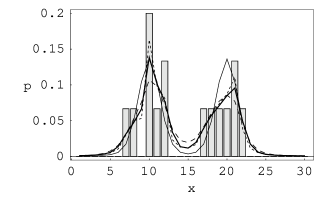
Figure 4: Bayesian reconstruction of potentials using the path integral method. Left part: original potential (thin line) and reconstructed potential (thick line). Right part: relative frequencies of sampled data (bars), likelihood of the true (thin line) potential and of the reconstructed potential: semiclassical density obtained by iteration (thick line), classical (dotted line) and quantum mechanical density (dashed line). Parameters: $\beta\,=\,10$, $m\,=\,1$, $\gamma\,=\,5$, $N\,=\,15$.

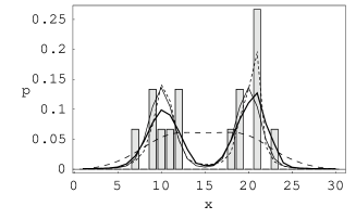
Figure 5: Bayesian reconstruction of potentials, using the path integral method, for small masses: Graphics as in Fig. 4. Parameters: $\beta\,=\,10$, $m\,=\,0.05$, $\gamma\,=\,10$, $N\,=\,15$.

for $\beta\,=\,10$. Eq. (4.6) is then solved, simultaneously with eqs. (8.4), (8.5), by iteration, using the gradient descent algorithm. The hyperparameter $\gamma$ is chosen such that the depths of the reconstructed potential and the true potential (8.10) are approximately equal as shown on the left hand side of Fig. 4. The right hand side shows the empirical density of data together with the likelihood for the true potential and for the classical, semiclassical and quantum mechanical reconstructions. For sufficiently heavy masses the gross shape of the potential is recognized; classical, semiclassical and quantum mechanical likelihoods are approximately the same. With decreasing mass, the differences of classical, semiclassical and quantum mechanical likelihoods become more pronounced, with the double–hump structure of the potential still recognized (Fig. 5). To better reproduce the absolute value of the potential minima one may decrease parameter $\gamma$ at the expense of distorting the symmetrical shape of the potential, like in Fig. 4.

9 Conclusion

In this paper we have developed the inverse problem of quantum statistics in path integral representation which supplements the energy representation used in a number of recent publications. The advantage of the path integral representation in this context turns out to be twofold: First, one can study the semiclassical and classical limits which are of interest for the analysis of experimental data as obtained from atomic force microscopy. Second, with the path integral representation for the likelihood and the functional integration over possible potential fields, one obtains a unified description for the basic equations of Bayesian inverse quantum statistics. Various approximation schemes have been studied for calculating, in this representation, the statistical operator and its derivatives which are the essential quantities in maximum posterior approximation. In particular, the classical limit is obtained and quadratic quantum fluctuations are calculated. A simple numerical example is presented to demonstrate the actual applicability of this approach which is expected to be useful for analysing experimental data when spatial distances are reached which resolve nanostructures like in recent atomic force microscopy.

Appendix

Matrix elements $\langle x^{\prime}|\mathrm{e}^{-\beta\,H}|x\rangle$ of the statistical operator and their functional derivatives with respect to $V$, needed in eq. (2.19), are easily calculated in energy representation. We start from the Schrödinger equation

$$H\,|\phi_{\alpha}\rangle\,=\,(T\,+\,V)\,|\phi_{\alpha}\rangle\,=\,E_{\alpha}\,|\phi_{\alpha}\rangle\,\,,$$ (A.1)

together with orthonormality and closure of eigenfunctions,

$$\langle\phi_{\alpha^{\prime}}|\phi_{\alpha}\rangle\,=\,\delta_{\alpha^{\prime}\alpha}\,\,,\qquad\sum\limits_{\alpha}\,|\phi_{\alpha}\rangle\,\langle\phi_{\alpha}|\,=\,{\rm 1\!l}\,\,.$$ (A.2)

For the derivatives of

$$\langle x^{\prime}|\mathrm{e}^{-\beta\,H}|x\rangle = \sum\limits_{\alpha}\,\langle x^{\prime}|\phi_{\alpha}\rangle\,\mathrm{e}^{-\beta\,E_{\alpha}}\,\langle\phi_{\alpha}|x\rangle$$ (A.3)

$$= \sum\limits_{\alpha}\,\phi^{*}_{\alpha}\,(x)\,\phi_{\alpha}\,(x^{\prime})\,\mathrm{e}^{-\beta\,E_{\alpha}}$$

and of

$$Z = \int dx\,\langle x|\mathrm{e}^{-\beta\,H}|x\rangle\,=\int dx\sum\limits_{\alpha}\,\langle x|\phi_{\alpha}\rangle\,\mathrm{e}^{-\beta\,E_{\alpha}}\,\langle\phi_{\alpha}|x\rangle$$ (A.4)

$$= \sum\limits_{\alpha}\int dx\,\phi^{*}_{\alpha}\,(x)\,\phi_{\alpha}\,(x)\,\mathrm{e}^{-\beta\,E_{\alpha}}\,=\,\sum\limits_{\alpha}\mathrm{e}^{-\beta\,E_{\alpha}}$$

we need $\delta\,E_{\alpha}\,/\,\delta\,v\,(x)$ and $\delta\,\phi_{\alpha}\,(x^{\prime})\,/\,\delta\,v\,(x)$. These derivatives are obtained by variation of the Schrödinger equation,

$$\frac{\delta\,H}{\delta\,V}\,|\phi_{\alpha}\rangle\,+\,H\,|\delta_{V}\,\phi_{\alpha}\rangle\,=\,\frac{\delta\,E_{\alpha}}{\delta\,V}\,|\phi_{\alpha}\rangle\,+\,E_{\alpha}\,|\delta_{V}\,\phi_{\alpha}\rangle$$ (A.5)

where, for a local potential $V\,(x^{\prime},\,x^{{}^{\prime\prime}})\,=\,v\,(x^{{}^{\prime\prime}})\,\delta\,(x^{\prime}\,-\,x^{{}^{\prime\prime}})$,

$$\langle x^{\prime}|\frac{\delta\,H}{\delta\,v\,(x)}|x^{{}^{\prime\prime}}\rangle\,=\,\frac{\delta\,H\,(x^{\prime},\,x^{{}^{\prime\prime}})}{\delta\,v\,(x)}\,=\,\delta\,(x^{\prime}\,-\,x^{{}^{\prime\prime}})\,\delta\,(x\,-\,x^{{}^{\prime\prime}})\,\,,$$ (A.6)

in short

$$\frac{\delta\,H}{\delta\,v\,(x)}=|x\rangle\,\langle x|\,\,.$$ (A.7)

Multiplying (A.5) by $\langle\phi_{\alpha}|$ from the left and using the adjoint of (A.1),

$$\langle\phi_{\alpha}|\,H\,=\,\langle\phi_{\alpha}|\,E_{\alpha}\,\,,$$ (A.8)

yields with normalization (A.2)

$$\frac{\delta\,E_{\alpha}}{\delta\,v\,(x)} = \langle\phi_{\alpha}|\frac{\delta\,H}{\delta\,V}|\phi_{\alpha}\rangle$$ (A.9)

$$= \langle\phi_{\alpha}|x\rangle\,\langle x|\phi_{\alpha}\rangle\,=\,|\phi_{\alpha}\,(x)|^{2}\,\,.$$

Hence our first result, in agreement with (5.3), is

$$\frac{\delta\,Z}{\delta\,v\,(x)} = -\beta\,\sum\limits_{\alpha}\,\mathrm{e}^{-\beta\,E_{\alpha}}\,\frac{\delta\,E_{\alpha}}{\delta\,v\,(x)}=-\beta\sum\limits_{\alpha}\,\mathrm{e}^{-\beta\,E_{\alpha}}\,|\phi_{\alpha}\,(x)|^{2}$$ (A.10)

$$= -\beta\,\sum\limits_{\alpha}\langle x|\phi_{\alpha}\rangle\,\mathrm{e}^{-\beta\,E_{\alpha}}\,\langle\phi_{\alpha}|x\rangle\,=\,-\beta\,\langle x|\mathrm{e}^{-\beta\,H}|x\rangle\,\,,$$

with closure (A.2).

To find the derivative of $\phi_{\alpha}\,(x^{\prime})$ with respect to $v\,(x)$ we rewrite (A.5) as inhomogeneous equation,

$$(E_{\alpha}\,-\,H)\,|\delta_{V}\,\phi_{\alpha}\rangle=\left(\frac{\delta\,H}{\delta\,V}-\frac{\delta\,E_{\alpha}}{\delta\,V}\right)|\phi_{\alpha}\rangle\,\,.$$ (A.11)

Obviously all orbitals $|\phi_{\alpha^{\prime}}\rangle$ with $E_{\alpha^{\prime}}\,=\,E_{\alpha}$ are in the null space of the operator $(E_{\alpha}\,-\,H)$, hence $(E_{\alpha}\,-\,H)$ is not invertible in full Hilbert space. However, the Moore-Penrose method of the pseudo-inverse can be applied to solve (A.11) for $|\delta_{V}\,\phi_{\alpha}\rangle$. The solvability condition states that the right hand side of (A.11) has no component in the null space of $(E_{\alpha}\,-\,H$). This is easily verified, multiplying (A.11) by $\langle\phi_{\alpha^{\prime}}|$ with $E_{\alpha^{\prime}}\,=\,E_{\alpha}$:

$$\langle\phi_{\alpha^{\prime}}|E_{\alpha}\,-\,H|\delta_{V}\,\phi_{\alpha}\rangle\,=\,0\,=\,\langle\phi_{\alpha^{\prime}}|\frac{\delta\,H}{\delta\,V}-\frac{\delta\,E_{\alpha}}{\delta\,V}|\phi_{\alpha}\rangle\,\,,$$ (A.12)

applying $H$ to the left according to (A.8). It is easy to control that

$$G_{\alpha}\,=\,\sum\limits_{\gamma\,\not=\,\alpha}\,\frac{|\phi_{\gamma}\rangle\langle\phi_{\gamma}|}{E_{\alpha}\,-\,E_{\gamma}}$$ (A.13)

is the pseudo-inverse of $(E_{\alpha}\,-\,H$), fulfilling the condition

$$G_{\alpha}\,(E_{\alpha}\,-\,H)\,G_{\alpha}\,=\,G_{\alpha}\,\,.$$ (A.14)

To obtain a unique solution of (A.11), or equivalently (A.5), we demand that $|\delta_{V}\,\phi_{\alpha}\rangle$ has no component in the null space of $(E_{\alpha}\,-\,H)$,

$$\langle\phi_{\alpha^{\prime}}|\delta_{V}\,\phi_{\alpha}\rangle\,=\,0\quad\text{for all}\quad\phi_{\alpha^{\prime}}\quad\text{with}\quad E_{\alpha^{\prime}}\,=\,E_{\alpha}\,\,.$$ (A.15)

This corresponds to fixing norm and phase of the eigenstates $|\phi_{\alpha}\rangle$ and, in case of degeneracy, uses the freedom to work with arbitrary orthonormal linear combinations of the respective eigenstates. Applying the pseudo-inverse $G_{\alpha}$ to (A.11) and using the orthonormality (A.2) we thus find in the subspace where $(E_{\alpha}\,-\,H$) is invertible

$$|\delta_{V}\,\phi_{\alpha}\rangle\,=\,\sum\limits_{\begin{array}[]{c}\scriptstyle{\gamma}\\ \scriptstyle{E_{\gamma}\,\not=\,E_{\alpha}}\end{array}}(E_{\alpha}\,-\,E_{\gamma})^{-1}\,|\phi_{\gamma}\rangle\,\langle\phi_{\gamma}|\delta_{V}\,H|\phi_{\alpha}\rangle\,\,,$$ (A.16)

or explicitly in coordinate representation with eq. (A.6)

$$\frac{\delta\,\phi_{\alpha}\,(x^{\prime})}{\delta\,v\,(x)}=\sum\limits_{\begin{array}[]{c}\scriptstyle{\gamma}\\ \scriptstyle{E_{\gamma}\,\not=\,E_{\alpha}}\end{array}}\frac{1}{E_{\alpha}\,-\,E_{\gamma}}\,\phi_{\gamma}\,(x^{\prime})\,\phi_{\gamma}^{*}\,(x)\,\phi_{\alpha}\,(x)\,\,.$$ (A.17)

With the derivatives (A.9) and (A.17), given in terms of the solutions of the Schrödinger equation, we can now construct the functional derivative of $\langle x^{\prime}|\mathrm{e}^{\beta\,H}|x\rangle$ with respect to $v\,(x^{{}^{\prime\prime}})$ according to (A.3):

$$\frac{\delta}{\delta\,v\,(x^{{}^{\prime\prime}})}\,\langle x^{\prime}|\mathrm{e}^{-\beta\,H}|x\rangle=-\beta\,\mathrm{e}^{-\beta\,E_{\alpha}}\sum\limits_{\alpha}\,\phi_{\alpha}^{*}(x)\,\phi_{\alpha}(x^{\prime})\,|\phi_{\alpha}\,(x^{{}^{\prime\prime}})|^{2}$$

(A.18)

$$+\!\!\!\sum\limits_{\begin{array}[]{c}\scriptstyle{\alpha,\,\gamma}\\ \scriptstyle{\alpha\,\not=\,\gamma}\end{array}}\frac{\exp(-\beta\,E_{\alpha})}{E_{\alpha}-E_{\gamma}}\left\{\phi_{\alpha}^{*}(x)\,\phi_{\gamma}(x^{\prime})\,\phi^{*}_{\gamma}(x^{{}^{\prime\prime}})\,\phi_{\alpha}(x^{{}^{\prime\prime}})+\phi_{\gamma}^{*}(x)\,\phi_{\gamma}(x^{{}^{\prime\prime}})\,\phi_{\alpha}^{*}(x^{{}^{\prime\prime}})\,\phi_{\alpha}(x^{\prime})\right\}.$$

In particular, for diagonal elements with $x^{\prime}\,=\,x$,

$$\begin{array}[]{c}\displaystyle{\frac{\delta}{\delta\,v\,(x^{{}^{\prime\prime}})}\,\langle x|\mathrm{e}^{-\beta\,H}|x\rangle\,=\,-\beta\,\mathrm{e}^{-\beta\,E_{\alpha}}\,\sum\limits_{\alpha}\,|\phi_{\alpha}\,(x)|^{2}\,|\phi_{\alpha}\,(x^{{}^{\prime\prime}})|^{2}}\\ \mbox{}\\ \displaystyle{+\!\!\sum\limits_{\begin{array}[]{c}\scriptstyle{\alpha,\,\gamma}\\ \scriptstyle{\alpha\,\not=\,\gamma}\end{array}}\,\frac{\exp\,(-\beta\,E_{\alpha})}{E_{\alpha}\,-\,E_{\gamma}}\,2\,\text{Re}\,\left\{\phi_{\alpha}^{*}\,(x)\,\phi_{\gamma}\,(x)\,\phi_{\alpha}\,(x^{{}^{\prime\prime}})\,\phi_{\gamma}^{*}\,(x^{{}^{\prime\prime}})\right\}}\end{array}$$ (A.19)

This result, eq. (A.19), is identical with (5.5) as can be shown by carrying out the $\beta^{\prime}$–integration in (5.5) using the energy representation of the matrix elements under the integral:

$$\begin{array}[]{c}\displaystyle{\frac{\delta\,\langle x|\mathrm{e}^{-\beta\,H}|x\rangle}{\delta\,v\,(x^{{}^{\prime\prime}})}\,=-\int\limits_{0}^{\beta}\!\!d\beta^{\prime}\,\langle x|\mathrm{e}^{-(\beta-\beta^{\prime})\,H}|x^{{}^{\prime\prime}}\rangle\langle x^{{}^{\prime\prime}}|\mathrm{e}^{-\beta^{\prime}\,H}|x\rangle\,=}\\ \mbox{}\\ \displaystyle{-\sum\limits_{\alpha,\,\gamma}\phi_{\alpha}(x)\,\phi^{*}_{\alpha}\,(x^{{}^{\prime\prime}})\,\phi_{\gamma}\,(x^{{}^{\prime\prime}})\,\phi_{\gamma}^{*}\,(x)\,\times\,\mathrm{e}^{-\beta\,E_{\alpha}}\int\limits_{0}^{\beta}\!\!d\beta^{\prime}\,\exp\,(-\beta^{\prime}\,(E_{\gamma}-E_{\alpha}))\,\,,}\end{array}$$ (A.20)

inserting the closure relation (A.2). With the $\beta^{\prime}$-integration carried out,

$$\int\limits_{0}^{\beta}\!\!d\beta^{\prime}\,\exp\,(-\beta^{\prime}\,(E_{\gamma}\,-\,E_{\alpha}))\,=\,\left\{\begin{array}[]{ccc}\beta&\text{for}&\alpha\,=\,\gamma\,\,,\text{or else}\\ \mbox{}\\ \displaystyle{\frac{1}{E_{\gamma}\,-\,E_{\alpha}}}&-&\displaystyle{\frac{\exp\,(-\beta\,(E_{\gamma}\,-\,E_{\alpha}))}{E_{\gamma}\,-\,E_{\alpha}}}\,\,,\end{array}\right.$$ (A.21)

one obtains

$$\begin{array}[]{c}\displaystyle{\frac{\delta\,\langle x|\mathrm{e}^{-\beta\,H}|x\rangle}{\delta\,v\,(x^{{}^{\prime\prime}})}\,=\,-\beta\,\mathrm{e}^{-\beta\,E_{\alpha}}\,\sum\limits_{\alpha}\,|\phi_{\alpha}\,(x)|^{2}\,|\phi_{\alpha}\,(x^{{}^{\prime\prime}})|^{2}}\\ \mbox{}\\ \displaystyle{+\sum\limits_{\begin{array}[]{c}\scriptstyle{\alpha,\,\gamma}\\ \scriptstyle{\alpha\,\not=\,\gamma}\end{array}}\frac{\exp\,(-\beta\,E_{\alpha})}{E_{\alpha}\,-\,E_{\gamma}}\,2\,\text{Re}\,\left\{\phi_{\alpha}\,(x)\,\phi_{\alpha}^{*}\,(x^{{}^{\prime\prime}})\,\phi_{\gamma}\,(x^{{}^{\prime\prime}})\,\phi^{*}_{\gamma}\,(x)\right\}\,\,,}\end{array}$$ (A.22)

q. e. d.

Figure 3: Comparison of classical, semiclassical and quantum mechanical likelihood. Upper left part: original potential $v\,(x)$. Upper right part: potential $u\,(x)\,=\,-v\,(x)$, to be used in (8.2); thin horizontal lines indicate range and energy of paths $q_{x}\,(\tau)$. Lower left part: classical (dotted line), semiclassical (full line) and quantum mechanical (dashed line) likelihoods. Lower right part: paths $q_{x}\,(\tau)$ for various $x$-values. Parameters used are $m\,=\,0.1$, $\beta\,=\,6$, $n_{\tau}\,=\,30$, $n_{x}\,=\,30$. (In the figure $\tau$ is denoted $t$.)

References

• [1] A. N. Tikhonov and V. Arsenin, Solution of Ill-posed Problems (John Wiley, New York, 1977); V. N. Vapnik, Statistical Learning Theory (John Wiley, New York, 1998); A. Kirsch, An Introduction to the Mathematical Theory of Inverse Problems (Springer Verlag, New York, 1996).
• [2] R. G. Newton, Inverse Schrödinger Scattering in Three Dimensions (Springer Verlag, Berlin, 1989)
• [3] K. Chadan, D. Colton, L. Päivärinta, and W. Rundell, An Introduction to Inverse Scattering and Inverse Spectral Problems (SIAM, Philadelphia, 1997); B. N. Zakhariev and V. M. Chabanov, Inverse Problems 13 (1997) R47–R79.
• [4] J. C. Lemm, Bayesian Field Theory (The Johns Hopkins University Press, Baltimore, 2003).
• [5] J. C. Lemm, J. Uhlig, and A. Weiguny, Phys. Rev. Lett. 84 (2000) 2068; The European Physical Journal B 20 (2001) 349; J. C. Lemm and J. Uhlig, Few Body Systems 29 (2000) 25; Phys. Rev. Lett. 84 (2000) 4517; J. C. Lemm, Phys. Lett. A 276 (2000) 19.
• [6] J. Zinn–Justin, Quantum Field Theory and Critical Phenomena (Clarendon Press, Oxford 1996); L. S. Schulman, Techniques and Applications of Path Integration (John Wiley, New York, 1981); J. W. Negele and H. Orland, Quantum Many–Particle Systems (Addison–Wesley, Redwood City, CA, 1988).
• [7] B. Gotsmann and H. Fuchs, Phys. Rev. Lett. 86 (2001) 1872
• [8] H. Römer and T. Filk, Statistische Mechanik (VCH, Weinheim, 1994)
• [9] R. F. Dashen, B. Hasslacher, and A. Neveu, Phys. Rev. D 10 (1974) 4114; H. Kleinert, Pfadintegrale (Wissenschaftsverlag, Mannheim, 1993)
Refer to caption