Quantum state transfer between fields and atoms
in Electromagnetically Induced Transparency

Abstract

We show that a quasi-perfect quantum state transfer between an atomic ensemble and fields in an optical cavity can be achieved in Electromagnetically Induced Transparency (EIT). A squeezed vacuum field state can be mapped onto the long-lived atomic spin associated to the ground state sublevels of the $\Lambda$-type atoms considered. The EIT on-resonance situation show interesting similarities with the Raman off-resonant configuration. We then show how to transfer the atomic squeezing back to the field exiting the cavity, thus realizing a quantum memory-type operation.

I
Introduction

If photons are known to be fast and robust carriers of quantum information, a major difficulty is to store their quantum state. In order to realize scalable quantum networks divincenzo quantum memory elements are required to store and retrieve photon states. To this end atomic ensembles have been widely studied as potential quantum memories lukin ; polzik . Indeed, the long-lived collective spin of an atomic ensemble with two ground state sublevels appears as a good candidate for the storage and manipulation of quantum information conveyed by light duan . Various schemes have been studied: first, the recent ”slow-” and ”stopped-light” experiments have shown that it was possible to store a light pulse inside an atomic cloud hau ; phillips in the Electromagnetically Induced Transparency (EIT) configuration harris . EIT is known to occur when two fields are both one- and two-photon resonant with 3-level $\Lambda$-type atoms, which allows one field to propagate without dissipation through the medium. However, the storage has only been demonstrated for classical variables so far.
On the other hand, the stationary mapping of a quantum state of light (squeezed vacuum) onto an atomic ensemble has been experimentally demonstrated, this time in an off-resonant Raman configuration polzik2 and in a single pass scheme. Squeezing transfer from light to atoms is also interesting in relation to ”spin squeezing” wineland and has been widely studied polzik3 ; kuzmich ; kozhekin ; vernac1 ; molmer ; dantan1 .
In this paper, unlike the single-pass approaches, we consider a cavity configuration, allowing a full quantum treatment of the fluctuations for the atom-field system vernac1 . We show that it is possible to continuously transfer squeezing, either in an EIT or Raman configuration, between a cloud of cold 3-level $\Lambda$-type atoms placed in an optical cavity and interacting with two fields: a coherent pump field and a broadband squeezed vacuum field.
The paper is organized as follows: Sec. II briefly describes the system, in Sec. III we develop a simplified model and study the conditions under which the squeezing transfer is optimal. Both EIT and Raman schemes result in a quasi-perfect transfer, which is not true for an arbitrary detuning. In Sec. IV we check that these conclusions are in agreement with full quantum calculations, evaluate the transfer robustness with respect to a detuning from two-photon resonance and generalize to the case of non-zero amplitude fields. Last, we present a simple readout scheme for the atomic squeezing in Sec. V: the squeezing stored in the atomic medium can be retrieved on the vacuum field exiting the cavity by switching off and on the pump field. The efficiency of the readout process is conditioned by the temporal profile of the local oscillator used to detect the outgoing vacuum field fluctuations, and can be close to 100% by an adequate choice of the local oscillator profile.

II Model system

II.1 Atom-fields evolution equations

The system considered in this paper is a set of $N$ $3$-level atoms in a $\Lambda$ configuration, as represented in Fig 1. On each transition $i\longrightarrow 3$ the atoms interact with one mode of the electromagnetic field, $A_{i}$ in an optical cavity ($i=1,2$). The detunings from atomic resonance are $\Delta_{i}$ and the cavity detunings $\Delta_{ci}$. The $3$-level system is described using $9$ collective operators for the $N$ atoms of the ensemble: the populations $\Pi_{i}=\sum\limits_{\mu=1}^{N}\left|i\right\rangle_{\mu}\left\langle i\right|_{\mu}$ ($i=1-3)$, the components of the optical dipoles $P_{i}$ in the frames rotating at the frequency of their corresponding lasers and their hermitian conjugates and the components of the dipole associated to the ground state coherence: $P_{r}=\sum\limits_{\mu=1}^{N}\left|2\right\rangle_{\mu}\left\langle 1\right|_{\mu}$ and $P_{r}^{\dagger}$.

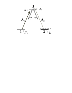
Figure 1: Three-level system in a $\Lambda$ configuration.

The atom-field coupling constants are defined by $g_{i}={\cal E}_{0i}d_{i}/\hbar$, where $d_{i}$ are the atomic dipoles, and ${\cal E}_{0i}=\sqrt{\hbar\omega_{i}/2\epsilon_{0}{\cal S}c}$. With this definition, the mean square value of a field is expressed in number of photons per second. To simplify, the decay constants of dipoles $P_{1}$ and $P_{2}$ are both equal to $\gamma$. In order to take into account the finite lifetime of the two ground state sublevels $1$ and $2$, we include in the model another decay rate $\gamma_{0}$, which is supposed to be much smaller than $\gamma$. Typically, the atoms fall out of the interaction area with the light beam in a time of the order of a few millisecond, whereas $\gamma$ is of the order of a few MHz for excited states. We also consider that the sublevels $1$ and $2$ are repopulated with in-terms $\Lambda_{1}$ and $\Lambda_{2}$, so that the total atomic population is kept constantly equal to $N$.

The system evolution is given by a set of quantum Heisenberg-Langevin equations

$$\dot{\Pi}_{1} = ig_{1}A_{1}^{\dagger}P_{1}-ig_{1}A_{1}P_{1}^{\dagger}+\gamma\Pi_{3}-\gamma_{0}\Pi_{1}+\Lambda_{1}+F_{11}$$

$$\dot{\Pi}_{2} = ig_{2}A_{2}^{\dagger}P_{2}-igA_{2}P_{2}^{\dagger}+\gamma\Pi_{3}-\gamma_{0}\Pi_{2}+\Lambda_{2}+F_{22}$$

$$\dot{\Pi}_{3} = -(ig_{1}A_{1}^{\dagger}P_{1}-ig_{1}A_{1}P_{1}^{\dagger})-(ig_{2}A_{2}^{\dagger}P_{2}-ig_{2}A_{2}P_{2}^{\dagger})$$

$$\hskip 85.35826pt-2\gamma\Pi_{3}+F_{33}$$

$$\dot{P}_{1} = -(\gamma+i\Delta_{1})P_{1}+ig_{1}A_{1}(\Pi_{1}-\Pi_{3})+ig_{2}A_{2}P_{r}^{\dagger}+F_{1}$$

$$\dot{P}_{2} = -(\gamma+i\Delta_{2})P_{2}+ig_{2}A_{2}(\Pi_{2}-\Pi_{3})+ig_{1}A_{1}P_{r}+F_{2}$$

$$\dot{P}_{r} = -(\gamma_{0}-i\delta)P_{r}+ig_{1}A_{1}^{\dagger}P_{2}-ig_{2}A_{2}P_{1}^{\dagger}+f_{r}$$

$$\dot{A}_{1} = -(\kappa+i\Delta_{c1})A_{1}+\frac{ig_{1}}{\tau}P_{1}+\sqrt{\frac{2\kappa}{\tau}}A_{1}^{in}$$

$$\dot{A}_{2} = -(\kappa+i\Delta_{c2})A_{2}+\frac{ig_{2}}{\tau}P_{2}+\sqrt{\frac{2\kappa}{\tau}}A_{2}^{in}$$

where $g_{1,2}$ are assumed real, $\delta=\Delta_{1}-\Delta_{2}$ is the two-photon detuning, $\kappa$ is the intracavity field decay and $\tau$ the round trip time in the cavity. The $F$’s are standard $\delta$-correlated Langevin operators taking into account the coupling with the other cavity modes. From the previous set of equations, it is possible to derive the steady state values and the correlation matrix for the fluctuations of the atom-fields system (see e.g. vernac1 ).

II.2 Decoupled equations for the fluctuations

In the case $\langle A_{2}^{in}\rangle=0$ and $\Lambda_{2}=N\gamma_{0}$, all the atoms are pumped in $|2\rangle$, so that only $\langle\pi_{2}\rangle$ is non zero in steady state. Here, we assume that $\langle A_{2}\rangle$ is zero, even if the number of intracavity photons is non-zero stricto sensu for a squeezed vacuum, this assumption is valid as long as the number of intracavity photons is much smaller than the number of atoms. In this case, the fluctuations for $\delta P_{r}$, $\delta P_{2}$ and $\delta A_{2}$ are then decoupled from the other operators fluctuations

$$\dot{\delta P_{r}} = -(\gamma_{0}-i\delta)\delta P_{r}+i\Omega\delta P_{2}+f_{r}$$ (1)

$$\dot{\delta P_{2}} = -(\gamma+i\Delta)\delta P_{2}+i\Omega\delta P_{r}+igN\delta A_{2}+F_{2}$$ (2)

$$\dot{\delta A_{2}} = -(\kappa+i\Delta_{c})\delta A_{2}+\frac{ig}{\tau}\delta P_{2}+\sqrt{\frac{2\kappa}{\tau}}\delta A_{2}^{in}$$ (3)

To simplify, we omit the subscript $2$ for $g$, $\Delta$ and $\Delta_{c}$, and assume that the Rabi pulsation associated to the pump field $\Omega=g_{1}\langle A_{1}\rangle$ is real. The atomic spin associated to the ground states is aligned along $z$ at steady state: $\langle J_{z}\rangle=\langle\pi_{2}-\pi_{1}\rangle/2=N/2$. We will place ourselves in this situation, which not only allows for analytical calculations and provides simple physical interpretations, but can also be generalized to arbitrary states for fields $A_{1}$ and $A_{2}$, as we will show further.
To characterize the quantum state of the atomic ensemble we look at the fluctuations of the spin components in the plane orthogonal to the mean spin: $J_{x}=(P_{r}+P_{r}^{\dagger})/2$ and $J_{y}=(P_{r}-P_{r}^{\dagger})/2i$. The spin component $J_{\theta}=J_{x}\cos\theta+J_{y}\sin\theta$ in the ($x,y$)-plane is said to be spin-squeezed when its variance is less than the coherent state value $|\langle J_{z}\rangle|/2$, and the degree of spin-squeezing is given by ueda

$$\Delta J^{2}_{min}=\min_{\theta}\frac{\Delta J^{2}_{\theta}}{|\langle J_{z}\rangle|/2}<1$$ (4)

III Adiabatical eliminations in the low frequency limit

III.1 EIT configuration

Since the ground state sublevels have a long lifetime compared to the excited state ($\gamma_{0}\ll\gamma$), and in the bad cavity limit ($\kappa\gtrsim\gamma$), the atomic spin associated to levels 1 and 2 evolves much slowly than the field or the optical coherence. Fourier-transforming Eqs. (1-2-3) and adiabatically eliminating $\delta P_{2}$ and $\delta A_{2}$, one gets a simplified equation for the ground state coherence fluctuations

$$\left[\gamma_{0}-i\delta+\frac{\Omega^{2}(\kappa+i\Delta_{c})}{d}-i\omega\right]\delta P_{r}(\omega)=$$ (5)

$$-\frac{gN\Omega}{d}\sqrt{\frac{2\kappa}{\tau}}\delta A_{2}^{in}(\omega)+\frac{i\Omega(\kappa+i\Delta_{c})}{d}F_{2}(\omega)+ f_{r}(\omega)$$

$$\text{with}\hskip 28.45274ptd=(\kappa+i\Delta_{c})(\gamma+i\Delta)+\frac{g^{2}N}{\tau}$$

In the so-called EIT configuration, the fields are one- and two-photon resonant: $\Delta=\delta=0$. Moreover, for the squeezing transfer to be optimal, one must have a zero-cavity detuning: $\Delta_{c}=0$ vernac1 ; dantan1 . The equations for the spin components in the ($x,y$)-plane are then

$$(\tilde{\gamma}_{0}-i\omega)\delta J_{x} = \frac{-gN\Omega}{\gamma(1+2C)\sqrt{T}}\delta A_{p}^{in}+\tilde{f}_{x}$$ (6)

$$(\tilde{\gamma}_{0}-i\omega)\delta J_{y} = \frac{-gN\Omega}{\gamma(1+2C)\sqrt{T}}\delta A_{q}^{in}+\tilde{f}_{y}$$ (7)

with an effective decay constant $\tilde{\gamma_{0}}=\gamma_{0}+\frac{\Gamma_{E}}{1+2C}$, $\Gamma_{E}=\Omega^{2}/\gamma$ being the one-photon resonant pumping rate. $T=2\kappa\tau$ is the coupling mirror transmission of the single-input cavity and $\tilde{f}_{x}$, $\tilde{f}_{y}$ are effective Langevin operators

$$\tilde{f}_{x}=f_{x}-\frac{\Omega}{\gamma(1+2C)}F_{y},\hskip 8.5359pt\tilde{f}_{y}=f_{y}+\frac{\Omega}{\gamma(1+2C)}F_{x}$$ (8)

$A_{p}=A_{2}+A_{2}^{\dagger}$ and $A_{q}=i(A_{2}^{\dagger}-A_{2})$ are the standard amplitude and phase quadratures for the squeezed vacuum field. Although the two modes $A_{1,2}$ do not need to be orthogonally polarized modes, it is rather convenient for the discussion to consider them as $\sigma_{+}$ and $\sigma_{-}$ modes of the field. In order to stress the similarity between the atomic spin and the Stokes vector which characterize the polarization state of the light, we introduce

$$S_{0} = \hskip 11.38092ptA_{1}^{\dagger}A_{1}+A_{2}^{\dagger}A_{2},\hskip 8.5359ptS_{y}=i(A_{1}^{\dagger}A_{2}-A_{1}A_{2}^{\dagger})$$

$$S_{x} = -(A_{1}^{\dagger}A_{2}+A_{1}A_{2}^{\dagger}),\hskip 5.69046ptS_{z}=A_{1}^{\dagger}A_{1}-A_{2}A_{2}^{\dagger}$$

The Stokes operators obey similar commutation relations $[S_{i},S_{j}]=2\epsilon_{ijk}S_{k}$ ($i=1,2,3$) similar to the atomic spin and therefore provide a useful and intuitive representation of the quantum state of the field in our situation. Since we assumed $\langle A_{2}\rangle=0$, the Stokes vector is parallel to the atomic spin: $\langle S_{z}\rangle=\langle A_{1}\rangle^{2}$ and $\langle S_{x}\rangle=\langle S_{y}\rangle=0$. Let us assume that the incident vacuum is squeezed for the amplitude quadrature $A_{p}$ and that the squeezing bandwidth is broad with respect to the cavity bandwidth, so that its minimal noise spectrum is $\langle(\delta A_{p}^{in})^{2}\rangle=e^{-2r}$. As $\delta S_{x}=-\langle A_{1}\rangle\delta A_{p}$, the field is also said to be $S_{x}$-polarization squeezed.

It is easy to see that the first terms in the r.h.s of (6-7) derive from an effective Hamiltonian

$$H_{E}=-\hbar\frac{2g^{2}}{\gamma(1+2C)\sqrt{T}}\left[J_{x}S_{y}^{in}-J_{y}S_{x}^{in}\right]$$ (9)

The Langevin forces in (6-7) being white noises, their contribution to the atomic noise is the same for any component in the ($x,y$)-plane. By looking at (6-7), one can see that, for a $S_{x}$-squeezed incident field, the least noisy spin component will be the $x$-component. Its normalized variance is

$$\Delta J_{min}^{2} = \frac{1}{|\langle J_{z}\rangle|/2}\left(\frac{1}{2\pi}\int d\omega\langle\delta J^{2}_{x}(\omega)\rangle\right)$$

$$= \frac{2C}{1+2C}\frac{\Gamma_{E}}{(1+2C)\tilde{\gamma}_{0}}e^{-2r}+\frac{\Gamma_{E}}{(1+2C)^{2}\tilde{\gamma}_{0}}+\frac{\gamma_{0}}{\tilde{\gamma}_{0}}$$

We used the fact that $\langle f_{x}(\omega)f_{x}(\omega^{\prime})\rangle=2\pi\delta(\omega+\omega^{\prime})\;N\gamma_{0}/2$ and $\langle F_{y}(\omega)F_{y}(\omega^{\prime})\rangle=2\pi\delta(\omega+\omega^{\prime})\;N\gamma/2$. The three terms in (III.1) can be understood as the coupling with the incident field ($\propto e^{-2r}$), the noise contribution of the optical dipole ($\propto\Gamma_{E}$) and the noise due to the loss of coherence in the ground state ($\propto\gamma_{0}$), respectively. We characterize the transfer efficiency as the ratio of the atomic squeezing created in the ground state to the incident field squeezing

$$\eta \equiv \frac{1-\Delta J_{min}^{2}}{1-e^{-2r}},$$

perfect transfer corresponding to $\eta=1$. In an ideal EIT configuration and in the lower frequency approximation, this parameter thus takes the form

$$\eta_{E}=\frac{2C}{1+2C}\frac{\Gamma_{E}/(1+2C)}{\gamma_{0}+\Gamma_{E}/(1+2C)}$$ (11)

The transfer is almost perfect - $\eta_{E}\sim 1$ - for a good cooperative behavior ($C\gg 1$) and when the effective EIT pumping is much larger than the loss rate in the ground state [$\Gamma_{E}/(1+2C)\gg\gamma_{0}$]. Note that, for a closed system ($\gamma_{0}=0$), the efficiency takes the extremely simple form

$$\eta_{max}=\frac{2C}{1+2C}\sim\frac{\text{Coupling}}{\text{Coupling+Atomic Noise}}$$

which emphasizes the central role played by the cooperativity to quantify the atom/field interaction in cavity. The noise degrading the transfer [$\propto 1/(1+2C)$] can thus be made very small with respect to the coupling [$\propto 2C/(1+2C)$] by increasing the cooperativity, i.e. for large atomic samples ($C\propto N$). In a cavity configuration, the cooperativity easily reaches 100-1000, ensuring in principle a perfect transfer.

III.2 Analogy with the Raman configuration

In a previous work dantan1 , we studied squeezing transfer in a $\Lambda$ system in the case where the fields are strongly detuned with respect to the atomic resonance ($\Delta_{1,2}\gg\gamma$). In such a configuration the three-level system can be reduced to an effective two-level system for the ground state. We denote the Raman optical pumping rate by $\Gamma_{R}=\gamma\Omega^{2}/\Delta^{2}$. When the effective two-photon detuning $\tilde{\delta}=\delta+\Omega^{2}/\Delta$, as well as the effective cavity detuning $\tilde{\Delta}_{c}=\Delta_{c}-g^{2}N/\Delta\tau$ are cancelled, the equations for the $x,y$-spin components read

$$(\tilde{\gamma}_{0}-i\omega)\delta J_{x} = +\frac{g^{2}N}{\Delta\sqrt{T}}\delta S_{y}^{in}+\tilde{f}_{x}$$ (12)

$$(\tilde{\gamma}_{0}-i\omega)\delta J_{y} = -\frac{g^{2}N}{\Delta\sqrt{T}}\delta S_{x}^{in}+\tilde{f}_{y}$$ (13)

with $\tilde{\gamma}_{0}=\gamma_{0}+(1+2C)\Gamma_{R}$ and

$$\tilde{f}_{x}=f_{x}-\frac{\Omega}{\Delta}F_{y},\hskip 8.5359pt\tilde{f}_{y}=f_{y}+\frac{\Omega}{\Delta}F_{x}$$ (14)

These equations were derived from the effective equations given in dantan1 by eliminating the intracavity field and introducing the incident Stokes vector as in the previous Section. As in EIT, one can deduce an effective Raman Hamiltonian

$$H_{R}=\hbar\frac{2g^{2}}{\Delta\sqrt{T}}\left[J_{x}S_{x}^{in}+J_{y}S_{y}^{in}\right]$$ (15)

Assuming again a $S_{x}$-squeezed incident field, the minimal variance is now that of the $y$-component, and one gets the following efficiency

$$\eta_{R}=\frac{2C}{1+2C}\frac{(1+2C)\Gamma_{R}}{\gamma_{0}+(1+2C)\Gamma_{R}}$$ (16)

The similarity between the EIT and Raman configuration appears clearly by comparing (6-7-8-11) to (12-13-14-16). The equations are formally identical by making the substitution

$$(1+2C)\gamma\longleftrightarrow\Delta$$ (17)

The important result is that the transfer efficiency takes the same form in both the on-resonant and strongly off-resonant situations

$$\eta = \frac{2C}{1+2C}\frac{\Gamma}{\gamma_{0}+\Gamma}$$

$$\text{with}\hskip 8.5359pt\Gamma=\frac{\Gamma_{E}}{1+2C}\hskip 8.5359pt\text{or}\hskip 8.5359pt(1+2C)\Gamma_{R}$$

The effective pumping rate, $\Gamma=\Gamma_{E}/(1+2C)$ or $(1+2C)\Gamma_{R}$, is obtained in each case by making the substitution (17), and can be made much larger than $\gamma_{0}$ with an adequate choice of $\Omega$. Note, however, that the EIT and Raman Hamiltonian are identical to a spin rotation by $\pi/2$ in the $(x,y)$-plane. We retrieve a well-known ”$\pi/2$” phase-shift phenomenon when going from ”on-resonance” to ”off-resonance”.

III.3 Transfer for an arbitrary detuning

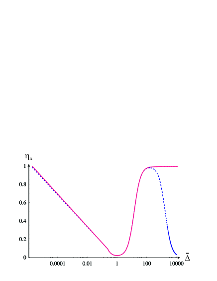
Figure 2: Transfer efficiency versus $\bar{\Delta}$ for $\gamma_{0}=0$ [plain] and $\gamma_{0}=\gamma/1000$ [dash] ($C=100$, $\gamma_{E}=15$).

The predictions given by the low frequency approximation in both the EIT and Raman configurations could lead one to expect squeezing transfer for any value of the one-photon detuning $\Delta$, provided one maintains the optimal transfer conditions $\tilde{\Delta}_{c}=\tilde{\delta}=0$. Moreover, given the $\pi/2$ rotation of the squeezed spin component when going over from on-resonance to off-resonance, one expects the squeezed component to continuously rotate from $0$ to $\pi/2$ when the detuning is increased.
Using (1-3-5) one finds the optimal transfer conditions to be

$$\tilde{\Delta}_{c} = \Delta_{c}-2C\kappa\frac{\gamma\Delta}{\gamma^{2}+\Delta}=0$$ (19)

$$\tilde{\delta} = \delta+\Gamma_{E}\frac{\gamma\Delta^{3}+(1-2C)\gamma^{3}\Delta}{(\gamma^{2}+\Delta^{2})[(1+2C)\gamma^{2}+\Delta^{2}]}=0$$ (20)

Eq. (5) then leads to the general equation for the spin component $J_{\theta}$ with angle $\theta$ in the $(x,y)$ plane

$$(\tilde{\gamma}_{0}-i\omega)\delta J_{\theta} = \alpha\delta A^{in}(\theta-\phi)$$

$$+\beta[e^{-i(\theta-\phi^{\prime})}F_{2}+e^{i(\theta-\phi^{\prime})}F_{2}^{\dagger}]/2$$

$$+[e^{-i\theta}f_{r}+e^{i\theta}f_{r}^{\dagger}]/2$$

with $\alpha$, $\beta$, $\tilde{\gamma}_{0}$, $\phi$ and $\phi^{\prime}$ functions depending on $\Delta$. Starting again with a $S_{x}$-squeezed field, the squeezed spin component will be $J_{\phi}$. After straightforward calculations the optimal efficiency for a given $\Delta$ is

$$\eta_{\Delta} = \frac{2C\gamma_{E}(1+\bar{\Delta}^{2})^{2}}{(1+2C+\bar{\Delta}^{2})}\times$$

$$\frac{1}{\sigma(1+\bar{\Delta}^{2})(1+2C+\bar{\Delta}^{2})+\gamma_{E}(1+(1+2C)\bar{\Delta}^{2})}$$

with $\sigma=\gamma_{0}/\gamma$, $\gamma_{E}=\Gamma_{E}/\gamma$ and $\bar{\Delta}=\Delta/\gamma$. This efficiency is plotted in Fig. 2 for the two cases considered previously: $\gamma_{0}=0$ and $\gamma_{0}\simeq 0$. In the first case the efficiency is optimal in EIT ($\bar{\Delta}=0$, $\eta_{\Delta}=\eta_{max}$), decreases to a minimum for $|\bar{\Delta}|=1$ ($\eta\sim 2/C\ll 1$) and increases again back to its maximal value $\eta_{max}$ when $\bar{\Delta}\gg 1$. The squeezed component angle can be shown to be $\theta_{sq}=\text{Arctan}\;\bar{\Delta}$, which varies as expected by $\pi/2$ when $\bar{\Delta}$ goes from 0 to infinity. One retrieves that the transfer is optimal either in an EIT or a Raman configuration. However, the transfer is really degraded in the intermediate regime $\bar{\Delta}\sim 1$.
If one takes into account losses in the ground state ($\gamma_{0}\neq 0$), the efficiency now reaches a maximum for $\bar{\Delta}\gg 1$

$$\eta_{\Delta} \simeq \eta_{max}\left(1-2\sqrt{\frac{\gamma_{0}}{\Gamma_{E}}}\right)\hskip 14.22636pt(C\gg 1,\;\gamma_{0}\ll\Gamma_{E})$$

for $$\bar{\Delta}\simeq\sqrt{2C}\left(\frac{\Gamma_{E}}{\gamma_{0}}\right)^{1/4}$$

before decreasing when the coupling in $(1+2C)\Gamma_{R}$ becomes too small as $\bar{\Delta}$ is increased ($\Omega$ being fixed) to compensate for the noise associated to the loss of coherence $\gamma_{0}$ [see Eq. (16)]. These effects stress the fragility of the squeezing transfer with respect to dissipation and explain why dissipation-less situations like EIT or Raman are favorable.

IV Full three-level calculation

From the Heisenberg-Langevin equations given at the beginning we calculated without approximation the spin covariance matrix and now compare it with the analytical model used in the previous Sections.

IV.1 Exact calculation in EIT

In the previous sections we neglected the frequencies larger than the atomic fluctuations evolution constant $\tilde{\gamma}_{0}$, assuming that $\kappa,\gamma\gg\tilde{\gamma}_{0}$. We therefore neglected high atom-field coupling frequencies due to the cavity. However, the analytical calculation of the minimal spin variance in EIT is possible using the Fourier transforms of (1-2-3). In EIT ($\Delta=\tilde{\Delta}_{c}=\tilde{\delta}=0$), the resulting equation for the $x$-component reads

$$\left[\gamma_{0}-i\omega+\frac{\Omega^{2}(\kappa-i\omega)}{D(\omega)}\right]\delta J_{x}=$$

$$+\frac{g^{2}N}{D(\omega)}\sqrt{\frac{2\kappa}{\tau}}\delta S_{x}^{in}+f_{x}- \frac{\Omega(\kappa-i\omega)}{D(\omega)}F_{y}$$

$$\text{with}\hskip 8.5359ptD(\omega)=(\kappa-i\omega)(\gamma-i\omega)+\frac{g^{2}N}{\tau}$$

If the incident field is $S_{x}$-squeezed, we know the $x$-component will be squeezed. However, a well-know coupling frequency ($\omega_{c}\simeq\sqrt{2C/\rho}\gamma$) appears at high frequency vernac1 , resulting in an increase of atomic noise, and, consequently, in a degradation of the atomic squeezing. After integration, the exact efficiency is

$$\eta_{E}= \frac{2C\gamma_{E}}{(1+2C)\sigma+\gamma_{E}}$$

$$\times \frac{1+\rho+\sigma\rho}{2C(1+\rho)+(1+\sigma)(1+\rho+\sigma\rho+\sigma\rho^{2}+\gamma_{E}\rho^{2})}$$

with $\gamma_{E}=\Gamma_{E}/\gamma$, $\rho=\gamma/\kappa$ and $\sigma=\gamma_{0}/\gamma$. Three regimes can be distinguished: for very small values of the effective pumping $\Gamma=\Gamma_{E}/(1+2C)$ compared to the loss rate in the ground state $\gamma_{0}$, one retrieves the low frequency (11) result as can be seen from Fig. 3: the efficiency is bad as long as the loss of coherence in the ground state $\gamma_{0}$ is not overcome by the pumping. In an intermediate regime $\gamma_{0}\ll\Gamma\ll\gamma,\kappa$ the efficiency reaches its maximum. The optimal pumping rate $\gamma_{E}^{*}$ can be shown to be proportional to $\sqrt{\sigma}$

$$\frac{\gamma_{E}^{*}}{1+2C}\simeq\frac{\sqrt{1+\rho}}{\rho}\sqrt{\sigma}\hskip 14.22636pt(C\gg 1,\sigma\ll 1)$$

in good agreement with the results shown in Fig. 3. For values of $\Gamma$ comparable to $\gamma$, $\kappa$, the efficiency is no longer well reproduced by the low frequency approximation, since the adiabatical eliminations are no longer valid. In this regime, the efficiency asymptotically reaches that of a closed system ($\gamma_{0}=0$), for which (IV.1) reduces to a monotonously decreasing function of $\gamma_{E}$

$$\eta_{E}^{0}=\frac{2C}{1+2C+\gamma_{E}\frac{\rho^{2}}{1+\rho}}$$ (24)

The optimal transfer is naturally obtained by making a compromise between the coupling and the atomic noise, and occurs in the intermediate regime II between regime I, for which the coupling is small and the atomic noise due to ground state coherence losses dominates, and regime III, in which the coupling is large, but the atomic noise due to spontaneous emission is more important.

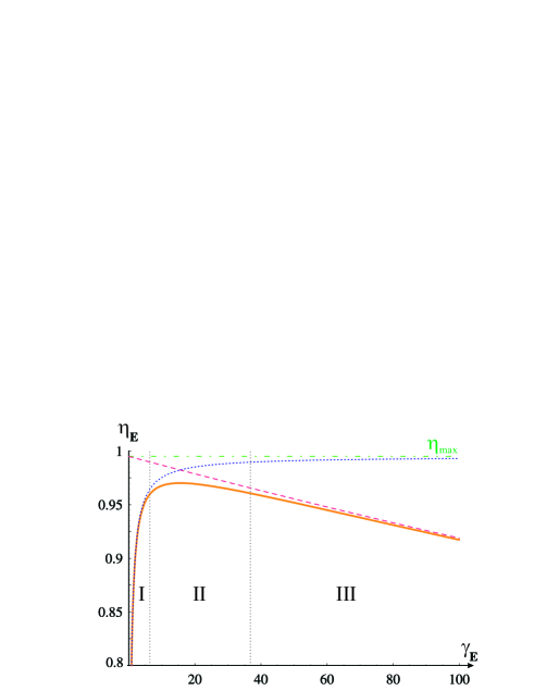
Figure 3: EIT Transfer efficiency versus EIT pumping rate: analytical (IV.1) [plain], low frequency approximation (11) [dots] and lossless system (24) [dashed]. The three regimes are I ($\Gamma\ll\gamma_{0}$), II ($\gamma_{0}\ll\Gamma\ll\gamma,\kappa$) and III ($\Gamma\gtrsim\gamma,\kappa$). Parameters: $C=100$, $\sigma=1/1000$, $\rho=1/2$. The optimal pumping rate is then $\gamma_{E}^{*}\simeq 15$.

IV.2 Robustness with respect to two-photon detuning

In a $\Lambda$ scheme, the coherence created between the ground state sublevels strongly depends on the two-photon resonance, the width of which is given by the effective atomic decay constant $\tilde{\gamma}_{0}$. In Fig. 4 we plot the transfer efficiency for the least noisy spin component as a function of the two-photon detuning for a zero-cavity detuning, that is, when (19) is fulfilled, but not (20). In addition to rotating the maximally squeezed component in the $(x,y)$-plane, the spin squeezing is clearly destroyed as soon as $\tilde{\delta}\sim\tilde{\gamma}_{0}$. We would like to emphasize that both EIT and Raman configurations are equally sensitive to this two-photon resonance condition. This similarity adds to the resemblance already stressed in Sec. III.2.

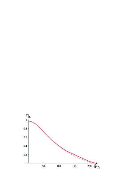
Figure 4: Transfer efficiency versus $\tilde{\delta}/\gamma_{0}$ in EIT [plain] and Raman [dash] schemes. Parameters: $C=100$, $\sigma=1/1000$, $e^{-2r}=0.5$. With these values, $\Gamma_{E}$ and $\Gamma_{R}$ are chosen so that, in both cases, $\tilde{\gamma}_{0}\simeq 75\gamma_{0}$.

IV.3 Transformation to the ”$\langle A_{2}\rangle=0$” basis

In this Section we show that any incident field state can actually be transferred to the atoms in EIT. To simplify the discussion let us assume again that the modes $A_{1,2}$ interacting with the transitions of the $\Lambda$ system are orthogonally polarized modes. Because of the similarities existing between the Stokes vector and the atomic spin, the results obtained in the special case $\langle A_{2}\rangle=0$ and $\langle J_{z}\rangle=N/2$ considered previously can be applied to any polarization state of the incident field. The Hamiltonian for a $\Lambda$ system in EIT reads

$$H=\hbar[g_{1}A_{1}^{\dagger}P_{1}+g_{2}A_{2}^{\dagger}P_{2}+\text{h.c.}]$$

If both $\langle A_{1}\rangle$ and $\langle A_{2}\rangle$ are non-zero, one can always turn to a basis $(A_{1}^{\prime},A_{2}^{\prime})$ for which $\langle A_{2}^{\prime}\rangle=0$ via a rotation R in the Poincaré sphere. The Hamiltonian is invariant under the same rotation performed on the atomic spin, the atoms are pumped into the dark state $|D\rangle=\textrm{R}|2\rangle$ and the $A^{\prime}_{2}$ field state will thus imprint on the atomic spin. Let us assume, for instance, that $A_{1}$ and $A_{2}$ have minimal noises $e^{-2r_{i}}$ for the same quadratures and take $\Omega_{i}=g_{i}\langle A_{i}\rangle$ ($i=1,2)$ as real numbers. The dark state is then

$$|D\rangle=\frac{-\Omega_{2}|1\rangle+\Omega_{1}|2\rangle}{\sqrt{\Omega_{1}^{2}+\Omega_{2}^{2}}}$$

The minimal atomic variance is then a weight of the $A_{1,2}$ modes squeezings

$$\Delta J^{2}_{min}\simeq\frac{\Omega_{2}^{2}e^{-2r_{1}}+\Omega_{1}^{2}e^{-2r_{2}}}{\Omega_{1}^{2}+\Omega_{2}^{2}}$$

One finds naturally that one cannot transfer more than the squeezing of one mode.

V Reading scheme and quantum memory

We have shown how the quantum state of the incident field could be transferred to the atomic spin in the ground state. Note that the lifetime associated to the ground state is quite long for cold atoms, and therefore the quantum information can be stored for a long time (several ms). Let us start with our spin squeezed atomic ensemble and switch off the fields at time $t=0$. The spin squeezing then decreases on a time scale given by the ground state lifetime $\gamma_{0}^{-1}$. After a variable delay, we rapidly switch on again the pump field, field $A_{2}^{in}$ being in a coherent vacuum state, and we look at the fluctuations of the field exiting the cavity $A^{out}_{2}=\sqrt{T}A_{2}-A_{2}^{in}$. Let us assume an EIT configuration for simplicity and start with a $J_{x}$-squeezed atomic spin; one expects its fluctuations to imprint on the $S_{x}$ component of the outgoing field [see (9)].

V.1 Standard homodyne detection

We assume a standard homodyne detection scheme with a constant local oscillator and calculate the noise power of $A^{out}_{q}$ measured by a spectrum analyzer integrating during a time $T_{0}$ over a frequency bandwidth $\Delta\omega$ centered around zero-frequency

$$P(t)=\int_{-\frac{\Delta\omega}{2}}^{\frac{\Delta\omega}{2}}\frac{d\omega}{T_{0}}\int_{t}^{t+T_{0}}d\tau\int_{t}^{t+T_{0}}d\tau^{\prime}e^{-i\omega(\tau-\tau^{\prime})}\mathcal{C}(\tau,\tau^{\prime})$$

where $\mathcal{C}(\tau,\tau^{\prime})=\langle\delta A_{p}^{out}(\tau)\delta A_{p}^{out}(\tau^{\prime})\rangle$ is the correlation function of $A_{p}^{out}$. Note that $T_{0}$ and $\Delta\omega$ must satisfy $T_{0}\Delta\omega\geq 2\pi$. In the low frequency approximation and in the ”good” regime for transfer ($\gamma_{0}\ll\Gamma_{E}/(1+2C)\ll\gamma,\kappa$; see Sec. IV.1), the correlation function of $A_{p}^{out}$ may be calculated via the Laplace-transforms of Eqs. (1-2-3)

$$\mathcal{C}(\tau,\tau^{\prime})=\delta(\tau-\tau^{\prime})-\frac{4C\Gamma_{E}}{(1+2C)^{2}}R_{at}e^{-\tilde{\gamma}_{0}(\tau+\tau^{\prime})}$$ (25)

where $R_{at}=1-\Delta J^{2}_{min}$ represents the atomic squeezing when the pump field is switched on again. After some algebra, one gets

$$\frac{1}{\Delta\omega}P(t)=1-S(a,b)R_{at}e^{-2\tilde{\gamma}_{0}t}$$

where $S$ is an integral depending on two dimensionless parameters: $a=T_{0}\tilde{\gamma}_{0}$ and $b=\Delta\omega/\tilde{\gamma}_{0}$, which, for large values of $C$, is equal to

$$S(a,b)=2\int_{-b/2}^{b/2}\frac{d\bar{\omega}}{ab}\frac{1+e^{-2a}-2e^{-a}\cos(\bar{\omega}a)}{1+\bar{\omega}^{2}}$$

with $\bar{\omega}=\omega/\tilde{\gamma}_{0}$. This integral, which can be understood as the signal-to-noise ratio of the readout process, is also the ratio of the measured field squeezing $R_{out}=1-P(0)/\Delta\omega$ to the initial atomic squeezing $R_{at}$. Squeezing may thus be transferred back from the atoms to the field. This squeezing decreases back to a coherent vacuum state on a time scale $\tilde{\gamma}_{0}^{-1}$ given by the atoms. $S(a,b)$ is optimal when the spectrum analyzer is Fourier-limited: $b=2\pi/a$, and when the time measurement is of the order of the inverse of the atomic spectrum width: $a\simeq 1.3$. Under these conditions, the integral is about 0.64, and about two-third of the atomic squeezing is transferred to the field exiting the cavity: $R_{out}\simeq 0.64R_{at}$.

V.2 Temporal matching

This imperfect readout comes from the fact that the local oscillator detecting the fluctuations of vacuum mode exiting the cavity is not perfectly matched with the atomic squeezing spectrum molmer . It is possible to reach a perfect readout by choosing the right temporal profile for the local oscillator: $E_{LO}(\tau)=e^{-\zeta\tilde{\gamma}_{0}\tau}$, with $\zeta$ a dimensionless adjustable parameter. The spectrum analyzer now measures

$$P(t)=\int_{-\frac{\Delta\omega}{2}}^{\frac{\Delta\omega}{2}}\frac{d\omega}{T_{0}} \int_{t}^{t+T_{0}}d\tau\int_{t}^{t+T_{0}}d\tau^{\prime}e^{-i\omega(\tau-\tau^{\prime})}$$

$$\times E_{LO}(\tau)E_{LO}(\tau^{\prime})\mathcal{C}(\tau,\tau^{\prime})$$

Using the correlation function (25), one gets

$$\frac{1}{\Delta\omega}P(t) = N(a,\zeta)-S(a,b,\zeta)e^{-2\tilde{\gamma}_{0}t}R_{at}$$

with $$N(a,\zeta)=\frac{1-e^{-2\zeta a}}{2\zeta a}$$

$$S(a,b,\zeta) = \frac{2}{ab}\int_{-b/2}^{b/2}d\bar{\omega}\frac{1+e^{-2a(1+\zeta)}-2e^{-a(1+\zeta)}\cos(a\bar{\omega})}{(1+\zeta)^{2}+\bar{\omega}^{2}}$$

$N(a,\zeta)$ represents the noise level in the absence of atomic squeezing and $S(a,b,\zeta)$ the amplitude of the atomic squeezing transferred to the field. The field squeezing can be expressed as

$$R_{out}(t)\equiv 1-\frac{P(t)}{\Delta\omega N(a,\zeta)}=\frac{S(a,b,\zeta)}{N(a,\zeta)}e^{-2\tilde{\gamma}_{0}t}R_{at}$$

and, for short times, the readout efficiency is $\mu\equiv R_{out}(0)/R_{at}=S(a,b,\zeta)/N(a,\zeta)$. This efficiency is optimized when the spectrum analyzer is Fourier limited and when the integration time is larger than the inverse of the atomic spectrum width: $b=2\pi/a$ and $a\gg 1$. In this case, one has $N(a,\zeta)\sim 1/(2a\zeta)$ and $S(a,b,\zeta)\sim 2/a(1+\zeta)^{2}$, so that the efficiency reads

$$\mu\sim\frac{4\zeta}{(1+\zeta)^{2}}$$

It is maximal and equal to 1 when $\zeta=1$, i.e. when the temporal profile of the local oscillator perfectly matches the atomic noise spectrum. It is thus possible to fully retrieve the atomic squeezing stored into the atoms in an EIT configuration. Note that the same results can be obtained in a Raman configuration, in the regime $\gamma_{0}\ll(1+2C)\Gamma_{R}\ll\gamma,\kappa$. In both schemes, to ensure that the retrieved squeezing indeed originates from the atoms, one may vary the delay between the switching on and off, and check the exponential decay of the squeezing with $\gamma_{0}$.

VI Conclusion

To conclude, we have shown that a quasi-ideal squeezing transfer should be possible between a broadband squeezed vacuum and the ground state spin of $\Lambda$-type atoms. The cavity interaction allows for good transfer Our results for a cavity configuration are consistent with those obtained in single pass schemes with thick atomic ensembles lukin ; polzik ; kuzmich ; kozhekin ; molmer , although efforts are still being conducted to develop a full free-space quantum treatment duan2 . The most favorable schemes are those minimizing dissipation, such as EIT or Raman dantan1 , for the fluctuations of the intracavity field imprint on the atomic spin, thus mapping the incident field state onto the atoms. The relevant physical parameter for the transfer efficiency is the cooperativity, which quantifies the collective spin-field interaction and which can be large in a cavity scheme. The mapping efficiency was evaluated taking into account possible losses in the ground state. Its robustness with respect to a detuning from the two-photon resonance is shown to be the same in EIT and in the Raman scheme. We also generalized the EIT results to the case in which both fields have non-zero intensity. The atomic squeezing is in this case a combination of the incident field squeezings. This is related to the fact that, in EIT, the atoms are pumped into a dark-state and the atomic medium is then transparent for a certain combination of the fields. Such a dark-state pumping was exploited for double-$\Lambda$ atoms in dantan2 to generate ”self spin-squeezing” using only coherent fields.

Last, we propose a simple reading scheme for the atomic state, allowing a quantum memory-type operation. When the pump field is switched back on, the outgoing vacuum is squeezed by the atoms, and the atomic squeezing can be fully transferred back by temporally matching the local oscillator used to detect the outgoing vacuum fluctuations with the atomic spectrum. To our knowledge, it is the first instance in which the conservation of quantum variables is predicted in an EIT scheme within a full quantum model.

References

- (1) D.P. Di Vincenzo, Fortschr. Phys. 48, 771 (2000).
- (2) M.D. Lukin, S.F. Yelin, and M. Fleischhauer, Phys. Rev. Lett. 84, 4232 (2000); M.D. Lukin and M. Fleischhauer, Phys. Rev. Lett. 84, 5094 (2000); M. Fleischhauer and M.D. Lukin, Phys. Rev. A 65, 022314 (2002). For a review, see M.D. Lukin, Rev. Mod. Phys. 75, 457 (2003).
- (3) J. Hald, J.L. Sørensen, C. Schori, and E.S. Polzik, Phys. Rev. Lett. 83, 1319 (1999); B. Julsgaard, A. Kozhekin, and E.S. Polzik, Nature 413, 400 (2001).
- (4) L.M. Duan, J.I. Cirac, P. Zoller, and E.S. Polzik, Phys. Rev. Lett. 85, 5643 (2000); L.M. Duan, M.D. Lukin, J.I. Cirac, and P. Zoller, Nature 414, 413 (2001).
- (5) S.E. Harris and L.V. Hau, Phys. Rev. Lett. 82, 4611 (1999); C. Liu, Z. Dutton, C.H. Behroozi, and L.V. Hau, Nature 409, 490 (2001).
- (6) D.F. Phillips, A. Fleischhauer, A. Mair, and R.L. Walsworth, and M.D. Lukin, Phys. Rev. Lett. 86, 783 (2001).
- (7) S.E. Harris, Phys. Today 50, 36 (1997).
- (8) C. Schori, B. Julsgaard, J.L Sørensen, and E.S. Polzik, Phys. Rev. Lett. 89, 057903 (2002).
- (9) D.J. Wineland, J.J. Bollinger, W.M. Itano, and D.J. Heinzen, Phys. Rev. A 50, 67 (1994).
- (10) A. Kuzmich, K. Mølmer, and E.S. Polzik, Phys. Rev. Lett. 79, 4782 (1997).
- (11) A. Kuzmich, L. Mandel, and N.P. Bigelow, Phys. Rev. Lett. 85, 1594 (2000).
- (12) L. Vernac, M. Pinard, and E. Giacobino, Phys. Rev. A 62, 063812 (2000); L. Vernac, M. Pinard, and E. Giacobino, Eur. Phys. J. D 17,125 (2001).
- (13) A.E. Kozhekin, K. Mølmer, and E.S. Polzik, Phys. Rev. A 62, 033809 (2000).
- (14) U.V. Poulsen and K. Mølmer, Phys. Rev. Lett. 87, 123601 (2001).
- (15) A. Dantan, M. Pinard, V. Josse, N. Nayak, and P.R. Berman, Phys. Rev. A 67, 045801 (2003).
- (16) M. Kitawaga and M. Ueda, Phys. Rev. A 47, 5138 (1993).
- (17) L.M. Duan, J.I. Cirac, and P. Zoller, Phys. Rev. A 66, 023818 (2002).
- (18) A. Dantan, M. Pinard, and P.R. Berman, Eur. Phys. J. D 27, 193 (2003).