Observation of Exceptional Points in Electronic Circuits

Abstract

Two damped coupled oscillators have been used to demonstrate the occurrence of exceptional points in a purely classical system. The implementation was achieved with electronic circuits in the kHz-range. The experimental results perfectly match the mathematical predictions at the exceptional point. A discussion about the universal occurrence of exceptional points – connecting dissipation with spatial orientation – concludes the paper.

A surprising phenomenon occurring in systems described by non-hermitian Hamiltonians has been observed in a number of experiments: the coalescence of two eigenmodes. If the system depends on some interaction parameter $\lambda\,,$ the value $\lambda_{\rm EP}$ at which the coalescence occurs is called an exceptional point (EP) Kato . At an EP, the eigenvalues and eigenvectors show branch point singularities Kato ; Hesa ; BerryEP ; Mondragon ; kors as functions of $\lambda\,.$ This stands in sharp contrast to two-fold degeneracies, where no singularity but rather a diabolic point BerryDP occurs. EPs have been described in laser induced ionization of atoms Latinne , in acoustical systems Shuva , and have actually been observed in microwave cavities BrentanoEP ; DemboEP ; DemboCh , in optical properties of certain absorptive media Pancha ; BerryPancha , and in “crystals of light” Oberthaler . The broad variety of physical systems showing EPs indicates that their occurrence is generic. So far EPs have been analyzed for the special case of a complex symmetric effective Hamiltonian he99 used for the description of dissipative wave mechanical systems such as in microwave cavities.

The physical interest in EPs is not only due to their universal occurrence in virtually all problems of matrix diagonalization. It is in particular the chiral character associated with the wave functions at the EP heha . This has been experimentally confirmed recently DemboCh and also thoroughly discussed in optics for anisotropic absorptive media beden . The fascinating point is the the wave function at the EP: not only is there – at the point of the two coalescing energies – one and only one state vector, but – for a complex symmetric matrix – its form is given by

$$|\psi^{+}_{{\rm EP}}\rangle=\begin{pmatrix}0\cr\vdots\cr i\cr 1\cr 0\cr\vdots\end{pmatrix}\quad{\rm or}\quad|\psi^{-}_{{\rm EP}}\rangle=\begin{pmatrix}0\cr\vdots\cr-i\cr 1\cr 0\cr\vdots\end{pmatrix}.$$ (1)

Only one EP of the pair is accessible in the laboratory as only one is associated with a negative sign of the imaginary part of the energy. The labels of the non-vanishing components in Eq.(1) are the labels of the two coalescing energies. Note that there is no parameter dependence; the form of the state vector is robust. We may associate this form with a circularly polarized wave. For a general non-hermitian matrix the ratio of the two relevant components is no longer $\pm i$ but an arbitrary complex number that can in general be associated with an elliptic polarisation beden .

In this letter we report the results of a plain classical experiment where an EP has been identified and so has the orientation that goes with it. It is the case of two coupled damped oscillators. This has been proposed in he03 for two mechanical oscillators. In the quoted paper a discussion of the EPs is extended to general matrices being no longer complex symmetric. In fact, the classical equations of motion for the momenta $p_{j}$ and coordinates $q_{j}$ read for the two mechanical oscillators

$$\frac{{\rm d}}{{\rm d}t}\begin{pmatrix}p_{1}\cr p_{2}\cr q_{1}\cr q_{2}\end{pmatrix}={\cal M}\begin{pmatrix}p_{1}\cr p_{2}\cr q_{1}\cr q_{2}\end{pmatrix}+\begin{pmatrix}c_{1}\cr c_{2}\cr 0\cr 0\end{pmatrix}\exp(i\omega t)$$ (2)

with

$${\cal M}=\begin{pmatrix}-2g-2k_{1}&2g&-f-\omega_{1}^{2}&f\cr 2g&-2g-2k_{2}&f&-f-\omega_{2}^{2}\cr 1&0&0&0\cr 0&1&0&0\end{pmatrix}$$ (3)

where $\omega_{j}-ik_{j},\;j=1,2$ are essentially the damped frequencies without coupling and $f$ and $g$ are the coupling spring constant and damping of the coupling, respectively. The driving force is assumed to be oscillatory with one single frequency and acting on each particle with amplitude $c_{j}$. Here we are interested only in the stationary solution being the solution of the inhomogeneous equation which reads

$$\begin{pmatrix}p_{1}\cr p_{2}\cr q_{1}\cr q_{2}\end{pmatrix}=(i\omega-{\cal M})^{-1}\begin{pmatrix}c_{1}\cr c_{2}\cr 0\cr 0\end{pmatrix}\exp(i\omega t).$$ (4)

Resonances occur for the real values $\omega$ of the complex solutions of the secular equation

$$\det|i\omega-{\cal M}|=0$$ (5)

and EPs occur for the complex values $\omega$ where

$${{\rm d}\over{\rm d}\omega}\det|i\omega-{\cal M}|=0$$ (6)

is fulfilled together with Eq.(5). Note that ${\cal M}$ is non-symmetric.

For easy implementation electronic circuits are used rather than the mechanical oscillators. The momenta and coordinates are replaced by voltage and current, respectively. The unperturbed undamped frequencies are given by $\omega_{j}^{2}=1/(L_{j}C_{j})$ with $L$ and $C$ being the inductance and capacitance, while damping and coupling are effected by resisters and mutual inductance. To allow for complex values of the effective inductance, resisters have been used in parallel to the inductance.

The actual experimental set-up is shown in Figure 1. The two circuit parameters that can be changed are the circuit capacitance $C_{p}$ and the parallel resistance $R_{p}$. Standard electronic components were used to construct the circuit. The component values are summarized in Table 1. The two inductors consist of multi-layer cylindrical air core windings wound onto PVC plastic coil formers. The coils are placed next to each other with their geometric axes aligned. The distance between them can be varied in order to change the coupling, i.e. the mutual inductance of the two coils.

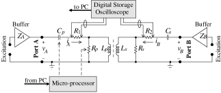
Figure 1: Measurement set-up.

Table 1: Component Values

Component	Value	Unit	Tolerance
$C_{p}$	65	nF	5 %
$R_{1}$	3.0	$\Omega$	10 %
$R_{p}$	520	$\Omega$	5 %
$L_{p}$	1.80	mH	5 %
$L_{s}$	2.55	mH	5 %
$R_{s}$	10.0	k$\Omega$	5 %
$R_{2}$	3.0	$\Omega$	10 %
$C_{s}$	47	nF	5 %
$M$	$0.14\sqrt{L_{p}L_{s}}=0.3$	mH	5 %

Input voltage signals $v_{A}$ and $v_{B}$ are connected to ports $A$ and $B$ of the circuit and are used to excite the system. The circuit response is given by the input currents $i_{A}$ and $i_{B}$ into ports $A$ and $B$, respectively. The two input currents can be determined by measuring the voltage drop over the series resistances $R_{1}$ and $R_{2}$. Using Ohm’s Law the currents can be calculated.

The input ports $A$ and $B$ of the circuit have to be excited by ideal voltage sources. In a practical set-up the excitation voltage sources must have output impedances, $Z_{A}$ and $Z_{B}$, that are much lower than the input impedances of the two circuit ports. The minimum input impedance of ports $A$ and $B$ are approximately $R_{1}$ and $R_{2}$, respectively. Buffers are used to reduce the signal impedance, such that $Z_{A}\ll R_{1}$ and $Z_{B}\ll R_{2}$.

A microprocessor is used to enable automatic multiple data collection. The microprocessor interfaces to a PC and varies the values of two circuit components $C_{p}$ and $R_{p}$. The input currents are measured with a digital oscilloscope. The oscilloscope is connected to the same PC as the microprocessor. The data from the oscilloscope is read directly into the PC where it is processed. The complete experiment is controlled with a software package called LabVIEW. A program written in LabVIEW is responsible for communicating with the microprocessor and the digital oscilloscope and processing the measurement data.

The first step in the measurement process is to determine the system Eigenvalues. The Eigenvalues can be determined from the system’s frequency response, i.e. the system’s spectrum. The frequency response $F_{A}(\omega)$ of the system at port $A$ is given by nilss

$$F_{A}(\omega)=\frac{I_{A}(\omega)}{V_{A}(\omega)}=\frac{\displaystyle\sum_{i=0}^{M}a_{i}\omega^{i}}{\displaystyle\sum_{i=0}^{N}b_{i}\omega^{i}}\,\,,$$ (7)

with $M\leq N$. Here $V_{A}(\omega)$ and $I_{A}(\omega)$ are the spectra of the applied voltage signal and the input current response at port $A$, respectively. A similar expression holds for the frequency response at port $B$. For the circuit in Figure 1, it is $N=M=4$. The resonance frequencies are the zeros of the denominator in Eq.(7).

The system’s frequency response can be determined by either performing measurements in the frequency or time domain. Time domain measurements yield more accurate results compared to frequency domain measurements. For a time domain measurement the system is excited by a short voltage pulse. The resulting response of the input current at a port is the impulse response of the system for that port. The Fourier transform of the impulse response is equal to the system’s frequency response. The frequency response depends on the measurement configuration, i.e. the port where the impulse response is measured and the relative amplitude of the excitation pulse at ports $A$ and $B$. In Eq.(7) only the roots of the numerator are dependent on the measurement configuration. The roots of the denominator, i.e. the eigenvalues, are independent of different measurement configurations.

In a practical set-up it is not possible to generate infinitely short pulses. However, the pulse width $t_{p}$ must be small compared to the response time of the system. A valid impulse response must obey

$$t_{p}\ll\frac{1}{\max(|\omega_{i}|)}\,\,,$$ (8)

with $\max(|\omega_{i}|)$ the eigenvalue with the largest modulus.

For this experiment both ports $A$ and $B$ where excited by the same voltage pulse. The input current into port $A$ was measured. Applying a Fourier transform to the measured impulse response current the frequency response of the system is obtained. By fitting Eq.(7) to the measured data the coefficients $a_{i}$ and $b_{i}$ can be determined and the resulting eigenvalues of the system calculated.

The measured eigenvalues for different values of $R_{p}$ and $C_{p}$ are plotted on the complex energy plane in Figure 2. Only two of the four eigenvalues of the system are plotted for each $R_{p}$ and $C_{p}$ value pair. The other two eigenvalues are mirrored with respect to the imaginary axis. Three resistance values were used, $R_{p}=430$, $R_{p}=470$ and $R_{p}=510$. For each resistance value the capacitance was changed from $57.0\,\mathrm{nF}$ to $72.0\,\mathrm{nF}$ in steps of $0.22\,\mathrm{nF}$. The resulting locus of eigenvalues repel from a point in the energy plane, which is the singular point of the system. The direction of each locus for an increasing value of $C_{p}$ is indicated in Figure 2. We denote the value of the frequency at the singular point by $S_{1}$ and find $S_{1}\approx 92000-i11500$ as indicated by a cross in Figure 2. A second singular point $S_{2}$ (not shown) is also measured and is mirrored with respect to the imaginary axis of the complex energy plane, i.e. $iS_{1}=(iS_{2})^{*}$. The measurement error is less than $6\,\%$.

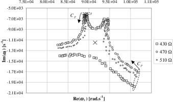
Figure 2: Measured system eigenvalues.

In order to measure the system phase, the system has to be excited with a steady-state sinusoidal signal. A real sinusoidal signal always consists of two frequency components $\omega_{1}$ and $\omega_{2}$ for which $i\omega_{1}=(i\omega_{2})^{*}$. Hence, to measure the system phase at the singular point, the system is excited with two complex frequencies equal to the two singular point values $S_{1}$ and $S_{2}$. Furthermore, the circuit values of $R_{p}$ and $C_{p}$ are set to obtain eigenvalues as close as possible to the two singular points. The excitation signals at port $A$ and $B$ have the form:

$$v(t)=C\sin(\omega_{0}t+\phi_{v})e^{-\gamma_{0}t}\,\,,$$ (9)

with $\omega_{0}=|\Re(S_{1})|=|\Re(S_{2})|$ and $\gamma_{0}=-\Im(S_{1})=-\Im(S_{2})$. The phase of the signal is $\phi_{v}$ and the amplitude $C$. For the measured system the value of $\gamma_{0}$ is positive ($\gamma\approx 11500\,s^{-1}$). This implies a decaying sinusoidal signal.

The aim of the experiment is to measure the steady-state phase difference $\Delta\phi_{i}$ between the two input currents $i_{A}$ and $i_{B}$. This is achieved by measuring the steady-state current response at the two ports simultaneously. The system is linear and the current response will have the same form as the excitation voltage in Eq.(9). The phase of the two input currents, $\phi_{iA}$ and $\phi_{iB}$, can be extracted by fitting Eq.(9) to each of the measured current responses. The amplitude and phase are the fitting parameters. The phase difference is then simply $\Delta\phi_{i}=\phi_{iA}-\phi_{iB}$.

However, the signal in Eq.(9) is not a power signal, i.e. it does not have a finite power content. It is therefore not possible in practice to generate such a signal. To perform the phase measurement the excitation is switched on at $t=t_{0}$. For $t<t_{0}$ the signal is zero. The on-set of the signal at $t=t_{0}$ introduces a decaying transient response. A reliable measurement of the steady-state phase can only be performed at $t-t_{0}\ll\gamma_{0}^{-1}$, where the transient response has decayed and can be neglected compared to the steady-state response.

To generate signals as described by Eq.(9) the circuit values of the circuit in Figure 1 were so chosen that singular points and eigenvalues are obtained within the audible frequency range. This enables the excitation signals to be generated with a standard computer sound card. LabVIEW is again used to drive the sound card of the PC and generate any arbitrary signal within the audible frequency range ($20\,\mathrm{Hz}$ to $20\,\mathrm{kHz}$). The stereo output of a computer sound card can be used to generate two different signals simultaneously.

Finally, the steady-state phase difference $\Delta\phi_{i}$ between the input currents was measured while exciting both ports. The phase difference $\Delta\phi_{v}$ between the two excitation signals was varied from 0 to $2\pi$ radians. In Figure 3 the measured current phase difference $\Delta\phi_{i}$ is plotted as a function of the excitation phase difference $\Delta\phi_{v}$. Also shown is the phase difference between the two input currents, $i_{A}$ and $i_{B}$, and the excitation voltage $v_{B}$ at port B. The measured phase difference $\Delta\phi_{i}$ is largely independent of the excitation phase difference $\Delta\phi_{v}$ with a value of approximately $\frac{\pi}{2}$ and a measurement error of $5\,\%$.

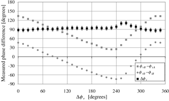
Figure 3: Measured system phase.

As far as the results are concerned we emphasize in particular two points: (i) the similarity of Fig.2 with the corresponding figure for instance in Latinne or DemboEP is striking; here it refers to electronic circuits, in the quoted papers to atomic physics or microwave cavities, respectively; (ii) the measured phase difference $\pi/2$ which is independent of the phase of the excitation, underlines once again the universal and robust chiral character of the state vector at the EP. We mention, that owing to the non-symmetric nature of the matrix considered (see Eq.(3)) there is in fact a slight deviation he03 . For the parameters chosen the precise quotient of the amplitudes actually is $-0.08+i1.99\ldots$ and not $i$ as in Eq.(1). In other words, there is a slight deviation from the circular toward an elliptic polarization. Yet an orientation prevails.

In this, like in all other experiments where EPs have been observed, dissipation is playing a foremost role. In fact, in quantum mechanics or optics, only absorption enables access in the laboratory to the singularity in the complex plane. And even in the experiment described in the present paper, where the underlying matrices are no longer symmetric, dissipation is crucial to give rise to an EP. The decay of the states provides a direction of the time axis. In classical and quantum systems absorption – and decoherence in the latter case legzu – occurs due to the interaction with the environment, the presence of the open channels is effectively described by complex interaction parameters he99 ; weid or, as in the present case, explicitly by Ohmic resisters.

In turn, the wave function at the EP is usually chiral in character as has been discussed in heha and confirmed experimentally the first time in DemboCh . We see here an intrinsic connection – provided by the mathematics of an EP – between the direction of time and a given direction in space. In fact, the present experiment can serve to define a direction in one dimensional space. At the EP, it is the one oscillator whose phase is leading while the phase of the other is lagging. These roles are fixed unequivocally for a given parameter set, unrelated to space. Viewing the oscillators placed along a straight line an orientation is defined along this line. This is not trivial and is caused by the mechanism at an EP: one, and only one-and-the-same oscillator has the leading phase, and this feature is cast in stone by a system that has no a priory spatial orientation. It is dissipation that brings about spatial orientation.

This does not mean, at this stage, that a classical set-up can provide a distinction between left and right. One is tempted to find a truly three-dimensional setting where one EP might do just that.

The authors ackowledge financial support by the South African National Research Foundation. They are grateful to H.B. Geyer for a critical reading of the manuscript.

References

- (1) T. Kato, Perturbation theory of linear operators (Springer, Berlin, 1966).
- (2) W.D. Heiss and A.L. Sannino, J. Phys. A 23, 1167 (1990); Phys. Rev. A 43, 4159 (1991).
- (3) M.V. Berry and D.H.J. O’Dell, J. Phys. A 31, 2093 (1998).
- (4) E. Hernández et al., J. Phys. A 33, 4507 (2000).
- (5) H.J. Korsch and S. Mossmann, J.Phys.A:Math.Gen. 36, 2139 (2003).
- (6) M.V. Berry and M. Wilkinson, Proc. R. Soc. Lond. A 392, 15 (1984).
- (7) O. Latinne et al., Phys. Rev. Lett. 74, 46 (1995).
- (8) A.L. Shuvalov and N.H. Scott, Acta Mech. 140, 1 (2000).
- (9) P.v. Brentano and M. Philipp, Phys. Lett. B 454, 171 (1999); M. Philipp et al., Phys. Rev. E 62, 1922 (2000).
- (10) C. Dembowski et al., Phys. Rev. Lett. 86, 787 (2001).
- (11) C Dembowski et.al., Phys. Rev. Lett. 90, 034101 (2003)
- (12) S. Pancharatnam, Proc. Ind. Acad. Sci. XLII, 86 (1955).
- (13) M.V. Berry, Curr. Sci. 67, 220 (1994).
- (14) M.K. Oberthaler et al., Phys. Rev. Lett. 77, 4980 (1996).
- (15) W.D. Heiss, Eur. Phys. J. D 7, 1 (1999); Phys. Rev. E 61, 929 (2000).
- (16) W.D. Heiss and H.L. Harney, Eur. Phys. J. D 17, 149 (2001).
- (17) M.V. Berry and M.R. Dennis, Proc.Roy.Soc. A 459, 1261 (2003).
- (18) W.D. Heiss, J.Phys.A: Mathematical and General, in press
- (19) J.W. Nilsson and S.A. Riedel, Electric Circuits, Addision Wesley, Massachusetts, 1996.
- (20) A.J. Leggett and W.H. Zurek in Fundamentals of Quantum Information, W.D. Heiss (Ed.), LNP587, Springer 2002
- (21) C. Mahaux and H.A. Weidenmuller Shell Model Approach to Nuclear Reactions, North-Holland, Amsterdam (1969).