Two-qubit Quantum Logic Gate in Molecular Magnets

Abstract

We proposed a scheme to realize a controlled-NOT quantum logic gate in a dimer of exchange coupled single-molecule magnets, $[\textrm{Mn}_{4}]_{2}$. We chosen the ground state and the three low-lying excited states of a dimer in a finite longitudinal magnetic field as the quantum computing basis and introduced a pulsed transverse magnetic field with a special frequency. The pulsed transverse magnetic field induces the transitions between the quantum computing basis so as to realize a controlled-NOT quantum logic gate. The transition rates between the quantum computing basis and between the quantum computing basis and other excited states are evaluated and analyzed.
PACS number(s): 03.67.Lx, 75.50.Xx, 75.10.Jm
Key words:Quantum computation, controlled-NOT gate, molecular magnets.

In recent years, quantum computation remarkably attracts the interests of the theoretical and experimental physicists because of its extensive prospects for the practical applications. With the development of the integration techniques, computational devices get smaller, eventually, the physical principles of quantum mechanics must be taken into account. The quantum algorithmsgrover ; shor discovered show that quantum computation is more effective than classical one. Many systems are investigated theoretically and experimentally to realize quantum computing, such as trapped ionscirac , solid state NMRgershenfeld ; cory , quantum dotsbarenco2 ; loss , SQUIDaverin ; makhin and spin clustersloss1 ; loss2 . Recently, quantum computation in molecular magnets is addressed. Leuenberger and Loss proposed a scheme to realize Grover’s algorithms in molecular magnets such as $\textrm{Fe}_{8}$ and $\textrm{Mn}_{12}$leuenberger .

Any quantum logic gate can be decomposed into one-qubit rotation and two-qubit controlled-NOT gate operationbarenco , so the key point for quantum computing is how to realize an arbitrary single-qubit operation gate and a two-qubit controlled-NOT gate(or controlled-phase gate), which are assembled together to realize a universal quantum computing. Realizing a two-qubit quantum logic gate in molecular magnets requires that there are interactions between different molecular particles. But for most molecular magnets such as $\textrm{Fe}_{8}$ and $\textrm{Mn}_{12}$, the interactions between molecules are relatively weak and have been neglected in most studies. Fortunately, the recent study of a dimerized single-molecule magnets, $[\textrm{Mn}_{4}]_{2}$, showed that intermolecular exchange interactions are not always negligiblewernsdorfer . This system is $[\textrm{Mn}_{4}\textrm{O}_{3}\textrm{Cl}_{4}(\textrm{O}_{2}\textrm{CEt})_{3}(\textrm{py})_{3}]_{2}$(called $[\textrm{Mn}_{4}]_{2}$), a member of the $[\textrm{Mn}_{4}\textrm{O}_{3}\textrm{Cl}_{4}(\textrm{O}_{2}\textrm{C}\textbf{R})_{3}(\textrm{py})_{3}]_{2}$ family, with $\textbf{R}=\textrm{Et}$. The supramolecular linkage within $[\textrm{Mn}_{4}]_{2}$ introduces exchange interactions between the $\textrm{Mn}_{4}$ molecules via the six C–H$\cdots$Cl pathways and the Cl$\cdots$Cl approach, which lead to noticeable antiferromagnetic coupling between the $\textrm{Mn}_{4}$ units. Each $\textrm{Mn}_{4}$ can be modelled as a ‘giant spin’ of $S=9/2$ with Ising-like anisotropy.

In this paper,we proposed a scheme to realize a controlled-NOT quantum logic gate in a dimer of exchange coupled single-molecule magnets. First, we don’t consider the transverse exchange interactions between two $\textrm{Mn}_{4}$ units, and choose the ground state and the three low-lying excited states as quantum computing basis. Then, we introduce an oscillating transverse magnetic field, which can induce transitions between the quantum computing basis so as to realize a controlled-NOT gate in molecular magnets. In our scheme, the two dipole-allowed transitions are at different resonance frequencies, while the oscillating magnetic field is in resonance with only one of them. Finally, we evaluate the amplitudes of transitions between quantum computing basis and the decaying rates of them due to the transverse exchange interactions.

The model– The corresponding Hamiltonian of each $\textrm{Mn}_{4}$ unit is given bywernsdorfer

$$H_{i}=DS_{zi}^{2}+g\mu_{B}B_{z}S_{zi},$$ (1)

where $i=1$ or $2$(referring to the two $\textrm{Mn}_{4}$ units of the dimer) , $D$ is the axial anisotropy constant, $\mu_{B}$ is the Bohr magneton, $S_{z}$ is the easy-axis spin operator, $g$ is the electronic g-factor, and $B_{z}$ is the applied longitudinal field. The last term in Eq.(1) is the Zeeman energy associated with an applied field. The $\textrm{Mn}_{4}$ units within $[\textrm{Mn}_{4}]_{2}$ are coupled by a weak superexchange via both the six C–H$\cdots$Cl pathways and the Cl$\cdots$Cl approach. Thus, the Hamiltonian of a dimer of exchange coupled molecular magnets, $[\textrm{Mn}_{4}]_{2}$, can be written aswernsdorfer

$$H_{dimer}=H_{1}+H_{2}+J_{z}S_{z1}S_{z2}+\frac{J_{xy}}{2}(S^{+}_{1}S^{-}_{2}+S^{-}_{1}S^{+}_{2}),$$ (2)

where $J_{z}$ and $J_{xy}$ are respectively the longitudinal and the transverse superexchange interaction constants, $S^{+}_{i}$ and $S^{-}_{i}$ are the usual spin raising and lowering operators respectively.

Firstly we don’t consider the transverse exchange interaction term in Eq.(2). Then the corresponding Hamiltonian can be simplified to the form

$$H_{0}=H_{1}+H_{2}+J_{z}S_{z1}S_{z2}.$$ (3)

For this simplification, every eigenstate of $[\textrm{Mn}_{4}]_{2}$ can be labelled by two quantum numbers $(m_{1},m_{2})$ for two $\textrm{Mn}_{4}$ units, with $m_{1}=9/2,7/2,\cdots,-9/2$ and $m_{2}=9/2,7/2,\cdots,-9/2$. The corresponding eigenvalues are given by

$$E^{(0)}_{m_{1}m_{2}}=(m_{1}^{2}+m_{2}^{2})D+(m_{1}+m_{2})g\mu_{B}B_{z}+m_{1}m_{2}J_{z},.$$ (4)

To realize a controlled-NOT gate, we introduce a pulsed time-depending transverse magnetic field $V(t)=B_{\bot}(t)[\cos(\omega t)\textbf{e}_{x}-\sin(\omega t)\textbf{e}_{y}]$, where $\textbf{e}_{x}$ and $\textbf{e}_{y}$ are respectively the unit vectors pointing along the $x$ and $y$ axes. Thus, we obtain the Hamiltonian due to the interactions with the transverse magnetic field asberman

$$H_{\bot}(t) = -\sum_{i}g\mu_{B}B_{\bot}(t)[\cos(\omega t)S_{xi}-\sin(\omega t)S_{yi}]$$ (5)

$$= -\sum_{i}\frac{g\mu_{B}B_{\bot}(t)}{2}[e^{i\omega t}S^{+}_{i}+e^{-i\omega t}S^{-}_{i}].$$

The pulsed transverse magnetic field rotates clockwise and thus produces left circularly polarized $\sigma^{-}$ photons. Absorption (emission) of $\sigma^{-}$ photons give rise to $\Delta m=-1(\Delta m=+1)$ transitions of spin states.

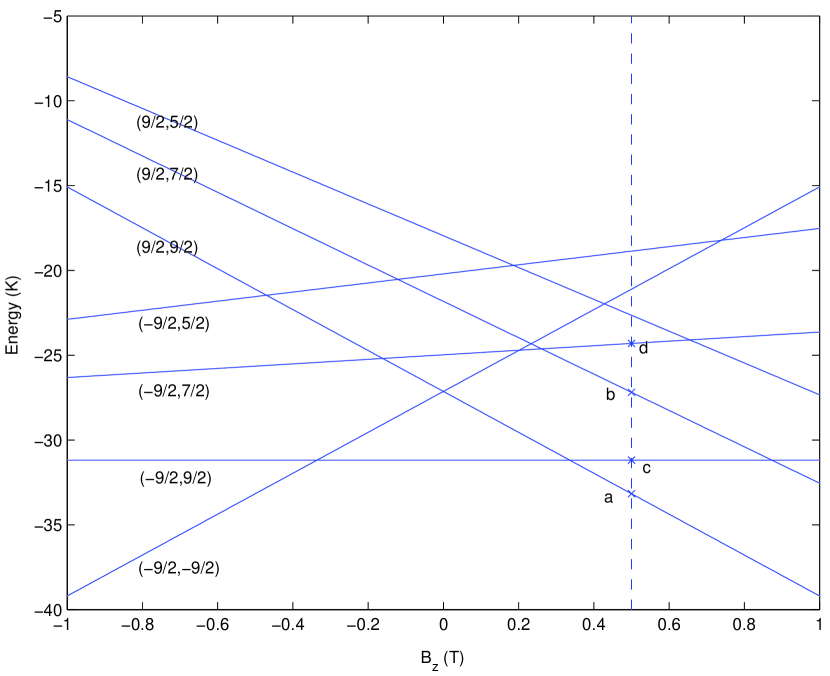
Figure 1: The spin states energies of $[\textrm{Mn}_{4}]_{2}$ for the low-lying states as a function of applied longitudinal magnetic field. The diagram is drawn according to the data calculated when $D=-0.72K$ and $J_{z}=0.1K$. Here, the states marked by the symbol $\times$ and labelled by the letters ‘a, b, c’ and ‘d’ are chosen as the quantum computing basis in our scheme.

A controlled-NOT gate– We choose the ground state and the three low-lying excited states in a finite longitudinal magnetic field as the basis for quantum computing, which are marked by the symbol ‘$\times$’ and labelled respectively by the letters ‘a,b,c’ and ‘d’ in Figure 1. These states are $(9/2,9/2),(9/2,7/2),(-9/2,9/2),(-9/2,7/2)$ in a 0.5T longitudinal magnetic field.

From the Eq.(4), we obtain the energy gaps between the quantum computing basis or between them and neighboring excited states, which are shown in Table 1. The energy gap $E^{(0)}_{-9/2,7/2}-E^{(0)}_{-9/2,9/2}$ between the states (-9/2,9/2) and (-9/2,7/2) is different from others, which is important to realize a controlled-NOT gate in our scheme.

Table 1: The energy gaps between the states chosen for quantum computing basis or between them and the neighboring excited states

Energy gaps between states	Values of energy gaps
$E^{(0)}_{-9/2,7/2}-E^{(0)}_{-9/2,9/2}$	$-8D-g\mu_{B}B_{z}+\frac{9}{2}J_{z}$
$E^{(0)}_{9/2,7/2}-E^{(0)}_{9/2,9/2}$	$-8D-g\mu_{B}B_{z}-\frac{9}{2}J_{z}$
$E^{(0)}_{-9/2,5/2}-E^{(0)}_{-9/2,7/2}$	$-6D-g\mu_{B}B_{z}+\frac{9}{2}J_{z}$
$E^{(0)}_{9/2,5/2}-E^{(0)}_{9/2,7/2}$	$-6D-g\mu_{B}B_{z}-\frac{9}{2}J_{z}$
$E^{(0)}_{7/2,9/2}-E^{(0)}_{9/2,9/2}$	$-8D-g\mu_{B}B_{z}-\frac{9}{2}J_{z}$
$E^{(0)}_{7/2,7/2}-E^{(0)}_{9/2,7/2}$	$-8D-g\mu_{B}B_{z}-\frac{7}{2}J_{z}$
$E^{(0)}_{7/2,9/2}-E^{(0)}_{9/2,7/2}$	$0$
$E^{(0)}_{-7/2,7/2}-E^{(0)}_{-9/2,9/2}$	$-16D+8J_{z}$
$E^{(0)}_{-7/2,5/2}-E^{(0)}_{-9/2,7/2}$	$-14D+7J_{z}$

Now we consider the pulsed transverse magnetic field introduced and evaluated the transition rates between the states by considering the Hamiltonian term about the transverse magnetic field, i.e. Eq.(5), as a perturbation. Using a rectangular pulse shapes with $B_{\bot}(t)=B_{\bot}$, if $-T/2<t<T/2$, and $0$ otherwise, we obtain the quantum amplitude for the transition from the state $(l,l^{\prime})$ to $(k,k^{\prime})$ induced by the magnetic field pulse,

$$C_{kk^{\prime};ll^{\prime}} = \frac{\pi g\mu_{B}B_{\bot}}{i\hbar}\sum_{i}\left[\langle kk^{\prime}|S^{+}_{i}|ll^{\prime}\rangle\delta^{(T)}(\omega_{kk^{\prime},ll^{\prime}}+\omega)+\langle kk^{\prime}|S^{-}_{i}|ll^{\prime}\rangle\delta^{(T)}(\omega_{kk^{\prime},ll^{\prime}}-\omega)\right]$$ (6)

where $\delta^{(T)}(\omega)={1}/{2\pi}\int_{-T/2}^{+T/2}e^{i\omega t}dt={\sin(\omega T/2)}/{\pi\omega}$ is the delta-function of the width $1/T$, ensuring overall energy conservation for $\omega T\gg 1$. For convenience, we denote the energy gaps between the quantum computing basis as $\omega_{1}=(E^{(0)}_{-9/2,7/2}-E^{(0)}_{-9/2,9/2})/\hbar$ and $\omega_{2}=(E^{(0)}_{9/2,7/2}-E^{(0)}_{9/2,9/2})/\hbar$. From the Table 1, we obtain $\Delta\omega\equiv\omega_{1}-\omega_{2}=9J_{z}/\hbar$. In our scheme, we choose the frequency of the magnetic pulse $\omega=\omega_{1}$. Then,the transition rate $w_{-9/2,7/2;-9/2,9/2}=|C_{-9/2,7/2;-9/2,9/2}|^{2}/T$ from the states $(-9/2,9/2)$ to $(-9/2,7/2)$ by absorbing a $\sigma^{-}$ photon is

$$w_{-9/2,7/2;-9/2,9/2}\simeq\frac{9T(g\mu_{B}B_{\bot})^{2}}{4\hbar^{2}},$$ (7)

where the relations $|\delta^{(T)}(\omega)|^{2}\approx(T/2\pi)\delta^{(T)}(\omega)$ and $\delta^{(T)}(0)=T/2\pi$ are used. The transition rate $w_{-9/2,9/2;-9/2,7/2}$ from the states $(-9/2,7/2)$ to $(-9/2,9/2)$ by emitting a $\sigma^{-}$ photon is identical to $w_{-9/2,7/2;-9/2,9/2}$. Since the magnetic pulse frequency $\omega$ isn’t equal to the energy gap $\omega_{2}$ between the states (9/2,9/2) and (9/2,7/2), i.e., $\omega_{1}\neq\omega_{2}$, which is shown in Figure 2, the transition rate between the two states is very small and can be negligible. From Reference wernsdorfer , the parameters $D$ and $J_{z}$ are chosen as $-0.72K$ and $0.1K$ respectively in this paper. We insert the parameters $T=10^{-8}\textrm{s}$ and $B_{\bot}=3.8\textrm{G}$ into Eq.(7) giving the transition rates $w_{-9/2,7/2;-9/2,9/2}=w_{-9/2,9/2;-9/2,7/2}=1.0\times 10^{8}\textrm{s}^{-1}$, while $w_{9/2,7/2;9/2,9/2}=w_{9/2,9/2;9/2,7/2}=2.4\times 10^{2}\textrm{s}^{-1}$. If we set $T=10^{-7}\textrm{s}$ and $B_{\bot}=0.38\textrm{G}$, then the transition rates $w_{-9/2,7/2;-9/2,9/2}=w_{-9/2,9/2;-9/2,7/2}=1.0\times 10^{7}\textrm{s}^{-1}$, while $w_{9/2,7/2;9/2,9/2}=w_{9/2,9/2;9/2,7/2}=0.23\textrm{s}^{-1}$. Here the values of $T$ and $B_{\bot}$ are chosen to guarantee $Tw_{-9/2,7/2;-9/2,9/2}=1$, i.e., the transverse magnetic pulse introduced is a $\pi$ pulse. From the data above, we can neglect the transitions between the states $(9/2,9/2)$ and $(9/2,7/2)$ compared with that between $(-9/2,9/2)$ and $(-9/2,7/2)$. In addition, the pulsed transverse magnetic field can induce transitions from the states as quantum computing basis to the other excited states, which lead to the decaying of quantum computing basis. When $T=10^{-8}\textrm{s}$ and $B_{\bot}=3.8\textrm{G}$, the transition rates $w_{-9/2,5/2;-9/2,7/2},w_{9/2,5/2;9/2,7/2}$ and $w_{7/2,7/2;9/2,7/2}$ are $4.4\times 10^{1}\textrm{s}^{-1},8.8\textrm{s}^{-1}$ and $3.6\times 10^{2}\textrm{s}^{-1}$ respectively; when $T=10^{-7}\textrm{s}$ and $B_{\bot}=0.38\textrm{G}$, transition rates $w_{-9/2,5/2;-9/2,7/2},w_{9/2,5/2;9/2,7/2}$ and $w_{7/2,7/2;9/2,7/2}$ are $2.5\times 10^{-2}\textrm{s}^{-1}$, $4.3\times 10^{-2}\textrm{s}^{-1}$ and $3.6\times 10^{-1}\textrm{s}^{-1}$ respectively. These transition rates are smaller several orders than the transition rates $w_{-9/2,7/2;-9/2,9/2}$ and $w_{-9/2,9/2;-9/2,7/2}$, so they are also negligible.

From the above discussion, we know that, when introducing the special frequency transverse magnetic field, only coherent transition between the spin states $(-9/2,9/2)$ and $(-9/2,7/2)$ is prominent and others are negligible. So we can interpret it as Rabi oscillation of two level atom. With $|a\rangle$ and $|b\rangle$ denote the spin states $(-9/2,9/2)$ and $(-9/2,7/2)$ respectively, simplify the Hamiltonian as

$$H_{rabi}(t) = \hbar\omega_{a}|a\rangle\langle a|+\hbar\omega_{b}|b\rangle\langle b|$$ (8)

$$-\frac{\hbar}{2}\Omega(e^{i\omega t}|a\rangle\langle b|+e^{-i\omega t}|b\rangle\langle a|).$$

where $\omega_{a}=E^{(0)}_{-9/2,9/2}/\hbar$, $\omega_{b}=E^{(0)}_{-9/2,7/2}/\hbar$ and $\Omega=g\mu_{B}B_{\bot}\hbar$ is Rabi frequency. The coherent wave function of the two states can be written in the form

$$|\psi(t)\rangle=c_{a}(t)e^{-i\omega_{a}t}|a\rangle+c_{b}(t)e^{-i\omega_{b}t}|b\rangle.$$ (9)

From Eqs.(8) and(9), we obtain the solution

$$c_{a}(t)=c_{a}(0)\cos\left(\frac{\Omega t}{2}\right)+ic_{b}(0)\sin\left(\frac{\Omega t}{2}\right),$$ (10)

$$c_{b}(t)=c_{b}(0)\cos\left(\frac{\Omega t}{2}\right)+ic_{a}(0)\sin\left(\frac{\Omega t}{2}\right),$$ (11)

where $c_{a}(0)$ and $c_{b}(0)$ are the initial values of $c_{a}$ and $c_{b}$ respectively when $t=0$. From this solution, we know that, if the transverse magnetic field introduced is $\pi$ pulse, i.e. $\Omega t=\pi$, we realize a NOT gate between the two states. Simultaneously, other states of computing basis do not vary.

Table 2: The comparisons of the physical quantum states and the quantum logic states of qubits for a controlled-NOT gate

Physical quantum states	Quantum logic states
$(9/2,9/2)\longrightarrow(9/2,9/2)$	$|00\rangle\longrightarrow|00\rangle$
$(9/2,7/2)\longrightarrow(9/2,7/2)$	$|01\rangle\longrightarrow|01\rangle$
$(-9/2,9/2)\longrightarrow(-9/2,7/2)$	$|10\rangle\longrightarrow|11\rangle$
$(-9/2,7/2)\longrightarrow(-9/2,9/2)$	$|11\rangle\longrightarrow|10\rangle$

Therefore,the pulsed magnetic field gives rise to the state transitions shown in the left column of Table 2. We choose the first $\textrm{Mn}_{4}$ unit as the control qubit and the second one as the target qubit. Here the quantum states $m_{1}=9/2$ and $-9/2$ of the first $\textrm{Mn}_{4}$ unit correspond to the quantum logic state $|0\rangle$ and $|1\rangle$ of the control qubit respectively, while the quantum states $m_{2}=9/2$ and $7/2$ of the second $\textrm{Mn}_{4}$ unit correspond to the quantum logic state $|0\rangle$ and $|1\rangle$ of the target qubit respectively, as shown in Table 2. In fact, the transition induced by the pulsed magnetic field correspond to the transform of the the quantum computing basis as

$$U_{CNOT}=\left(\matrix{1&0&0&0\cr 0&1&0&0\cr 0&0&0&1\cr 0&0&1&0}\right).$$ (12)

So our scheme has realized a conditional quantum dynamics in a dimer of exchange coupled single-molecule magnets, $[\textrm{Mn}_{4}]_{2}$.

In our scheme a key point is that the frequency of the pulsed transverse magnetic field is chosen as $\omega=\omega_{1}$ instead of $\omega=\omega_{2}$. Seemingly, if we choose the quantum states $m_{1}=-9/2$ and $9/2$ of the first $\textrm{Mn}_{4}$ unit as the quantum logic states $|0\rangle$ and $|1\rangle$ of the control qubit respectively and the frequency of the pulsed transverse magnetic field as $\omega=\omega_{2}$, the controlled-NOT gate can also be realized. However, this is not true. In fact, when $\omega=\omega_{2}$, the pulsed transverse field can induce the transition from the state $(9/2,9/2)$ to the states $(9/2,7/2)$ or $(7/2,9/2)$ by absorbing a $\sigma^{-}$ photon, because the states $(9/2,7/2)$ and $(7/2,9/2)$ are energy degenerate and the energy gaps $E^{(0)}_{9/2,7/2}-E^{(0)}_{9/2,9/2}$ and $E^{(0)}_{7/2,9/2}-E^{(0)}_{9/2,9/2}$ are identical with each other, which are shown in Table 1. Thus, if we choose $\omega=\omega_{2}$, the state $(9/2,9/2)$ will decay into the state $(7/2,9/2)$, which does not belong to the quantum computing basis.

The effects of the transverse exchange interactions– In the above discussion, we have not considered the transverse exchange interactions, i.e., the last term in Eq.(2), re-denoted as

$$H_{xy}=\frac{J_{xy}}{2}(S^{+}_{1}S^{-}_{2}+S^{-}_{1}S^{+}_{2})$$ (13)

which in fact can induce the decaying of the quantum computing basis into other excited states. In the first order, $H_{xy}$ acts between the zeroth-order eigenvectors $(m_{1},m_{2})$ and $(m_{1}\pm 1,m_{2}\mp 1)$. The effect of $H_{xy}$ on the tunnelling of the states is discussed in details in Ref.hill . We perturbatively evaluated the amplitude of the transition from the states from $(l,l^{\prime})$ to $(k,k^{\prime})$ as,

$$C_{kk^{\prime};ll^{\prime}}=\frac{2\pi}{i\hbar}\langle kk^{\prime}|H_{xy}|ll^{\prime}\rangle\delta^{(T)}(\omega_{kk^{\prime},ll^{\prime}})$$ (14)

Here the transitions from the quantum computing basis to other excited states induced by the $H_{xy}$ are $(9/2,7/2)\rightarrow(7/2,9/2),\;(-9/2,9/2)\rightarrow(-7/2,7/2)$ and $(-9/2,7/2)\rightarrow(-7/2,5/2)$, while transition from the state $(9/2,9/2)$ can not occur since the total spin of the $\textrm{Mn}_{4}$ unit is $9/2$. Since the superexchange interaction of the dimer $[\textrm{Mn}_{4}]_{2}$ is nearly isotropictiron , we set the parameter $J_{xy}=0.1K$. When the duration $T$ is infinite, $\delta^{(T)}(\omega_{kk^{\prime},ll^{\prime}})$ in Eq.(14) becomes Dirac delta function $\delta(\omega_{kk^{\prime},ll^{\prime}})$. The energy conservation holds when the transitions happen. From Table 1, only the transition between spin states $(9/2,7/2)$ and $(7/2,9/2)$ is possible. However, if $T$ is finite, the energy conservation does not hold during transition due to uncertainty principle. Thus, the transition between nondegenerate states is possible if $T$ is finite. Because the time of quantum computing operation is finite, it is necessary to evaluate the transition rate due to exchange interaction to compare with transition induced by magnetic field. When $T$ is $10^{-8}\textrm{s}$, we evaluated the transition rates $w_{7/2,9/2;9/2,7/2}$, $w_{-7/2,7/2;-9/2,9/2}$ and $w_{-7/2,5/2;-9/2,7/2}$ are $8.9\times 10^{-13}\textrm{s}^{-1}$, $3.8\times 10^{-21}\textrm{s}^{-1}$ and $1.3\times 10^{-20}\textrm{s}^{-1}$ respectively. If the duration $T=10^{-7}\textrm{s}$, then $w_{7/2,9/2;9/2,7/2}=8.9\times 10^{-12}\textrm{s}^{-1}$, $w_{-7/2,7/2;-9/2,9/2}=6.2\times 10^{-22}\textrm{s}^{-1}$ and $w_{-7/2,5/2;-9/2,7/2}=1.1\times 10^{-21}\textrm{s}^{-1}$. The rates of transitions induced by the transverse exchange interactions are far smaller than that of the transitions between the quantum computing basis, so we can neglect them and do not consider their effects in our scheme.

Conclusion– We have proposed a scheme to realize a controlled-NOT quantum logic gate in a dimer of exchange coupled single-molecule magnets, $[\textrm{Mn}_{4}]_{2}$. We first neglected the transverse exchange interactions between the two $\textrm{Mn}_{4}$ units and obtained the spin states, and the energy spectrum. Then, we chosen the ground state and the three low-lying excited states in a finite longitudinal magnetic field as the quantum computing basis and introduced a pulsed transverse magnetic field with a special frequency, which can induce transitions between the quantum computing basis so as to realize a controlled-NOT operation. In our scheme, the magnetic pulse is a $\pi$ pulse, which leads to the transitions of spin states with $\Delta m=\pm 1$. We have evaluated the transition rates induced by the transverse exchange interactions and analyzed the their effects on decaying of the states. In this paper, we have not considered the initializing, read-in and read-out of the states, which are needed to improve in technique for molecular magnets. If the measure approach of the single molecular magnet is improved, molecular magnets are promising candidates for quantum computing.

This work is in part supported by NSF of China No.10447125.

Figure 2: The schematic diagram for energy levels of a dimer $[\textrm{Mn}_{4}]_{2}$ without(the left hand) and with(the right hand) exchange interactions between two $\textrm{Mn}_{4}$ units. In the diagram, ‘a, b, c’ and ‘d’ refer to the states in Figure 1 labelled by ‘a, b, c’ and ‘d’ respectively, which are the quantum computing basis in our scheme. Here $\omega_{0}$ and $\omega_{1},\omega_{2}$ are the energy gaps between the quantum computing bases without and with exchange interactions respectively, and $\omega_{J}=9J_{z}/2\hbar$ refers to the energy shift due to exchange interactions.

References

• (1) L. K. Grover, Phys. Rev. Lett. 79,325(1997).
• (2) P. W. Shor, Proceeding of the 35th Annual symposium on the Foundations of Computer Science (IEEE Computer Society, Los Alamitos, CA)p.124(1994).
• (3) J. I. Cirac and P. Zoller Phys. Rev. Lett. 74,4901(1995).
• (4) N. A. Gershenfeld, I. L. Chuang, and S. Llyod, in PhysComp96: Proceedings of the Fourth Workshop on Physics and Computation, edited by T.Toffoli, M.Biafore, and J.Leão(New England Complex Systems Institute, Cambrigde, MA),p.136(1996).
• (5) D. G. Cory, D. G. Fhamy, and T. F. Havel, Pro. Natl. Acad. Sci. U.S.A 94, 1634(1997).
• (6) A. Barenco, D. Deutsch, A. Ekert, and R. Jozsa, Phys. Rev. Lett. 74, 4083(1995).
• (7) D. Loss and D. P. DiVincenzo Phys. Rev. A 57, 120(1998).
• (8) D. V. Averin, Solid state Commun. 105, 659(1998).
• (9) Y. Makhin, G. Sch’́on, and A. Shnirman, Rev. Mod. Phys. 73, 357(2001).
• (10) F. Meier, J. Levy, and D. Loss, Phys. Rev. Lett. 90, 047901(2003)
• (11) F. Meier, J. Levy, and D. Loss, Phys. Rev. B 68,134417(2003)
• (12) M. N. Leuenberger and D. Loss, Nature 410, 789(2001).
• (13) A. Barenco, C. H. Bennett, R. Cleve, D. P. DiVincenzo, N. Margolus, P. W. Shor, T. Sleator, J. A. Smolin, and H. Weinfurter, Phys. Rev. A 52,3457(1995).
• (14) W. Wernsdorfer, N. Aliaga-Alcalde, D. N. Hendrichson, and G. Christou, Nature 416, 406(2002).
• (15) G. P. Berman, D. K. Campbell, G. D. Doolen, G. V. López, and V. I. Tsifrinovich, Physica B 240, 61(1997).
• (16) S. Hill, R. S. Edwards, N. Aliaga-Alcalde, and G. Chistou, Science 302, 1015(2003).
• (17) R. Tiron, W. Wernsdorfer, D. Foguet-Albiol, N. Aliaga-Alcalde, and G. Christou Phys. Rev. Lett. 91, 227203 (2003)
Refer to caption