Control of Raman lasing in the non-impulsive regime

Abstract

We explore coherent control of stimulated Raman scattering in the non-impulsive regime. Optical pulse shaping of the coherent pump field leads to control over the stimulated Raman output. A model of the control mechanism is investigated.

Since the advent of pulsed lasers, there has been extensive experimental and theoretical work on stimulated Raman scattering. More recently there has been a resurgence of interest in impulsive Raman scatteringYan et al. (1985); Weiner et al. (1990); Nazarkin and Korn (1998); Bartels et al. (2002) due in part to the development of the field of learning coherent controlJudson and Rabitz (1992); Warren et al. (1993); Rabitz et al. (2000), along with advances in ultrafast laser technologyBackus et al. (1998) and programmable pulse shapingWefers and Nelson (1995); Tull et al. (1997). In the impulsive regime, the laser bandwidth is large compared to the frequency of the Raman mode (typically a molecular vibration). In the time domain the pulse duration is short compared to the vibrational period, and one can shape the optical pulse to drive molecular mode(s) on resonanceWeinacht et al. (2001). Alternatively, if the laser bandwidth contains photon pairs separated by the Stokes frequency, then the Raman gain can be seeded by the pump laser. Control of the Raman gain can be achieved by appropriately phasing colors in the pump pulse.

For the case of two-photon atomic absorption, this control mechanism has been described as shaping of the nonlinear power spectrum of the driving fieldMeshulach and Silberberg (1998); Bucksbaum (1998); Meshulach and Silberberg (1999). The idea has since been extended to multi-photon absorption in molecules Walowicz et al. (2002); Lozovoy et al. (2003), as well as vibrational Raman excitation in multi-mode molecular systemsWeinacht et al. (2001). Here again analysis leads to an explanation of the control via the nonlinear power spectrum of the pump pulse.

In the non-impulsive regime, the laser bandwidth is small compared to the frequency of the mode. Since there are no photon pairs separated by Stokes frequency in the pump pulse, the Stokes field must build up from spontaneous Raman scattering. This produces a Stokes field whose phase is random and cannot be controlled. Control may still be possible over the stimulated output spectrum or the final state populations in the presence of multiple Raman modes. Non-impulsive control of the stimulated Raman spectrum in liquid methanol has been reported in experiments that used learning algorithms to discover the optimal driving field Pearson et al. (2001, 2002). Here we demonstrate a possible mechanism for this control.

The details of our adaptive learning technique and laser system have been described previously Pearson et al. (2001). In learning control experiments, the physical system is used to find the optimal driving field (pulse shapes) without prior knowledge of the Hamiltonian Judson and Rabitz (1992). These solutions can be analyzed later to learn about the underlying quantum dynamics. Briefly, our experiments use a shaped, ultrafast Ti:Sapphire laser system as the excitation source. The laser pulses are shaped in an acousto-optic Fourier filter Tull et al. (1997) interfaced with a computer. Our spectral bandwidth ($4-5$ THz) and pulse shaping characteristics provide temporal control over the pulses ranging from $100$ fs to $5$ ps in duration. Our adaptive learning algorithm determines the pulse shapes by optimizing a feedback signal derived from the Raman spectrum.

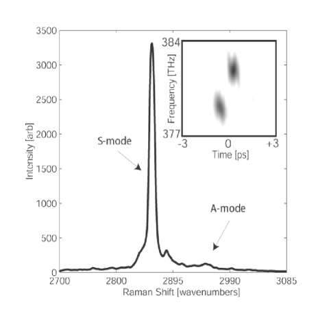
Figure 1: Resulting Raman spectra obtained after optimization with the feedback algorithm. Inset shows a Husimi plot of the optimal “double-blob” pulse shape that led to S-mode excitation.

The system under investigation in these experiments is liquid phase methanol (CH₃OH). We focus on the two C-H stretch vibrational modes labelled S ($2834$ cm^-1) and A ($2946$ cm^-1) Shimanouchi (1972). The experiments are performed in a $10$ cm liquid cell, and the forward scattered Raman spectrum is collected and fed back to the algorithm. The learning algorithm is able to channel the gain into either of the two Raman modes. Although the algorithm finds a variety of pulse shapes that produce the desired effect, one class of solutions stands out. Figure 1 (inset) shows a representative pulse shape of this class of solutions in the form of an optical Husimi distributionHillery et al. (1984). The Husimi plot is a two-dimension convolution of the Wigner functionHillery et al. (1984); Cohen (1989); Paye (1992) of the pulse shape that approximates the intensity distribution in both time and frequency. The optimal pulse shapes found by the algorithm consist of a pair of nearly transform-limited “blobs” that are separated by approximately $3.3$ THz. This energy splitting matches the S-A mode spacing. Figure 1 shows the resulting Raman spectrum after excitation by the pulse shown in the inset of Fig. 1. The pulse produces strong selective excitation of the S vibrational mode.

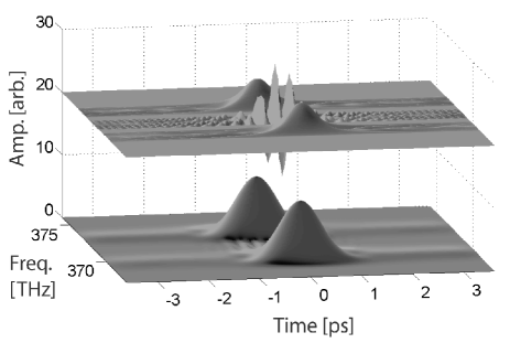
Figure 2: Calculated Wigner plots for double-blob pulse used in the experiment when the phase offset between the blobs is equal to $\pi$. The lower plot is the Husimi distribution when the phase offset is zero.

These two-blob solutions suggest a quasi-impulsive model for the interaction, where the pump field directs the Raman gain through a coherent coupling between the two modes Pearson et al. (2001). This coherence modulates the intensity envelope of the pulse. The modulation is apparent in the Wigner distribution, but has only a minimal effect on the Husimi distribution (Fig. $2$).

In order to study the effect of the phase offset, we excite the molecules with the original pulse shape shown in Fig. 2. We then collect the stimulated Raman spectra as the phase offset between the two blobs is varied from $0$ to $\pi$.

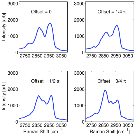
Figure 3: Stimulated Stokes output as a function of the Raman shift from the central frequency of the pump pulse. The different panels show the output spectra for various phase offsets. The gain oscillates between the S- and A-modes.

Figure 3 shows the stimulated Raman output spectrum for several different phase offsets. As the offset is varied, the Raman gain oscillates between the two different Stokes modes. As is to be expected, this single parameter control is not as effective at mode selection as the full learning algorithm (see Fig. 1). Nevertheless, control is achieved by varying only the phase offset. Care was taken to adjust the laser intensity to avoid saturation of the Raman gain, since this leads to significant changes in the observed control.

A simple model that predicts the observed effect can be constructed by expanding on previous work on single mode Raman scattering. The theory governing stimulated Raman gain of a single active mode under excitation by an off-resonant pump pulse has been developed both semi-classically Carman et al. (1970) and quantum mechanically Raymer and Mostowski (1981); Raymer and Walmsley (1990). In the quantum case, the Stokes field in the non-impulsive regime is generated by spontaneous fluctuations of the Raman polarizability. A number of approximations can be made to reveal the underlying physics. In the standard treatment, one assumes one-dimension, plane-wave pulse propagation in the slowly-varying envelope approximation (SVEA), and the calculation is performed in the transient regime where damping can be neglected. The pulse durations ($0.1$ to $1$ ps) imply that the SVEA is valid. The assumption of transient scattering may be an oversimplification because the pulse lengths approach the decoherence times of the C-H vibrationsIwaki and Dlott (2000). With these simplifications, the interaction can be reduced to a set of coupled differential equations describing the propagation along $\hat{z}$ of three fields inside the medium Lewenstein (1984):

$$\frac{\partial}{\partial x}\varepsilon_{L}=-q\varepsilon_{S},$$ (1)

$$\frac{\partial}{\partial x}\varepsilon_{S}=q^{*}\varepsilon_{L},$$ (2)

$$\frac{\partial}{\partial\tau}q=\frac{1}{4}\varepsilon_{L}\varepsilon_{S}^{*}.$$ (3)

In these equations, $\varepsilon_{L}$ is the pump laser field, $\varepsilon_{S}$ is the Stokes field, and $q$ is the molecular polarizability. The independent variables $x\propto z$ and $\tau\propto(t-z/c)$ are the reduced space-time coordinates.

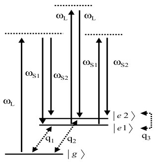
Figure 4: Energy level diagram with two Raman-active vibrational modes. The three levels are Raman coupled by the pump ($\omega_{L}$) and Stokes ($\omega_{S1}$ and $\omega_{S2}$) fields. The interaction generates coherences between pairs of the three levels ($q_{1}$, $q_{2}$, and $q_{3}$). An additional interaction is included by allowing a two-photon Raman coupling between the two excited vibrational states driven by either the applied pump field or the generated Stokes fields.

We have extended this treatment to include two vibrational Raman modes which, in addition to the original coupling to the same ground state, are Raman coupled to each other through two-photon transitions driven by the applied pump field or the generated Stokes fields. The relevant energy levels are shown in Fig. 4, where $|e1\rangle$ and $|e2\rangle$ are the first excited levels of the two vibrational modes. Equations 4 through 9 are the modified equations governing the optical fields and molecular polarizabilities in the case of two modes,

$$\frac{\partial}{\partial x}\varepsilon_{L} = -\varepsilon_{S1}q_{1}-\varepsilon_{S2}q_{2}-\frac{1}{4}\varepsilon_{L}q_{3}+\frac{1}{4}\varepsilon_{L}q_{3}^{*},$$ (4)

$$\frac{\partial}{\partial x}\varepsilon_{S1} = \varepsilon_{L}q_{1}^{*}+\frac{1}{4}\varepsilon_{S2}q_{3}^{*},$$ (5)

$$\frac{\partial}{\partial x}\varepsilon_{S2} = \varepsilon_{L}q_{2}^{*}-\frac{1}{4}\varepsilon_{S1}q_{3},$$ (6)

$$\frac{\partial}{\partial\tau}q_{1} = -\varepsilon_{L}\varepsilon_{S1}^{*}w_{1}-\imath\alpha\varepsilon_{L}\varepsilon_{L}^{*}q_{2}$$ (7)

$$-\imath\varepsilon_{L}\varepsilon_{S2}^{*}q_{3}-\imath\varepsilon_{S2}\varepsilon_{S1}^{*}q_{2},$$

$$\frac{\partial}{\partial\tau}q_{2} = -\varepsilon_{L}\varepsilon_{S2}^{*}w_{2}+\imath\alpha\varepsilon_{L}\varepsilon_{L}^{*}q_{1}$$ (8)

$$-\imath\varepsilon_{L}\varepsilon_{S1}^{*}q_{3}^{*}+\imath\varepsilon_{S1}\varepsilon_{S2}^{*}q_{1},$$

$$\frac{\partial}{\partial\tau}q_{3} = \imath\varepsilon_{S2}\varepsilon_{L}^{*}q_{1}+\imath\varepsilon_{L}\varepsilon_{S1}^{*}q_{2}^{*}$$ (9)

$$-\varepsilon_{L}\varepsilon_{L}^{*}(w_{1}-w_{2})$$

$$-\varepsilon_{S2}\varepsilon_{S1}^{*}(w_{1}-w_{2}).$$

In these equations, the $q_{i}$’s are the molecular coherences for the Raman-active transitions, the $w_{i}$’s represent the population inversion in each of the two modes, and $\alpha$ is a constant that describes the relative strength of the additional Raman coupling. Specifically, we include the quasi-impulsive pump-pump coupling, where the relative phase, $\phi_{L}$, appears implicitly in the terms containing $\varepsilon_{L}\varepsilon_{L}^{*}$. Finally, although substantial energy conversion between pump and Stokes fields is possible, the populations of the excited states in our experiments are always much less than the ground state, so terms in the calculation involving the off-diagonal coupling between the two excited states ($q_{3}$) may be suppressed.

In order to compare our model to the experimental results, we numerically integrate the set of coupled differential equations that describe the propagation of the fields inside the medium (see Eqs. 4 through 9). We set the amplitudes of the initial coherences ($q_{1}$ and $q_{2}$) to be small random numbers, which in turn determine the initial values of the Stokes phases $\phi_{S1}$ and $\phi_{S2}$. The equations are integrated over an interaction region comparable to the experimental conditions. At the end of the interaction length we calculate the total energy contained in each of the Raman fields as we vary the phase offset $\phi_{L}$ in our model pump pulse.

We expect the initial phases of the Stokes fields to be random because they buildup from spontaneous scattering. The stimulated Stokes field emerging from the methanol cell is clearly multimode, based on its angular divergence and far field appearance. When the excitation volume corresponds to a large value of the Fresnel number ($F=A/\lambda_{S}L$), such multiple spatial modes are excited, leading to a large number of independent SRS processes in each laser shotRaymer et al. (1985); Scalora and Haus (1992).

The high number of spatial modes implies multiple sets of initial phases for the two different Stokes frequencies on every laser pulse. Therefore we perform the integration over many trials of random initial amplitudes of the coherences $q_{1}$ and $q_{2}$ (using a white Gaussian noise about zero). The control comes from the $\varepsilon_{L}\varepsilon_{L}^{*}$ terms in the equations for the temporal derivatives of $q_{i}$. The physical picture is that the pump pulse drives the coherences $q_{i}$, which in turn drive the Stokes modes $\varepsilon_{S1}$ and $\varepsilon_{S2}$. Changing the value of $\phi_{L}$ in the equations changes which mode receives a positive contribution and which receives a negative. When the phase offset $\phi_{L}$ goes through $\pi/2$, the role of the two modes switches.

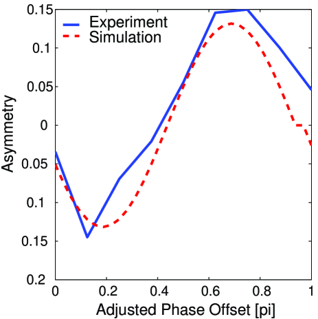
Figure 5: Variation in mode excitation as a function of phase shift between the two spectral regions for both experiment (solid) and simulation (dashed). The vertical axis plots the difference in the mode excitation divided by the sum. The simulation results have been adjusted to the data using two parameters: the initial phase of the field and the coupling strength between the two excited states.

We define the mode asymmetry as the ratio of the difference in energy between the two modes divided by the sum of the energy in the two modes. Although for a given initial pair ($q_{1}$,$q_{2}$) the mode asymmetry can take on any value between $\pm 1$, on average one of the modes is preferentially excited at each value of $\phi_{L}$. Figure 5 shows the effect of mode switching for the results from both the experiment and simulation. The mode asymmetry is plotted along the vertical axis. We find that both the experiment and simulation show a variation in mode excitation with similar periods. The simulation results have been adjusted to the data using two parameters: the pump-pump Raman coupling strength ($\alpha$) and the initial phase offset $\phi_{L}$. The depth of modulation in the asymmetry increases as the Raman coupling strength increases (the plot shows the result with $\alpha=7$). Changing the phase offset $\phi_{L}$ simply shifts the phase of the modulation. The phase offset in the experiment is unknown due to pulse propagation effects within the liquid. The mode control was relatively insensitive to the other parameters of the model, which were set to approximate experimental values of the Raman threshold.

In conclusion, we have demonstrated mode selection in stimulated Raman scattering in liquid methanol through control of the coherence of the pump laser. Control is possible even though the pump laser bandwidth is insufficient to seed the Stokes waves. Using our feedback control results as a starting point, we have constructed a simple model of the process that could explain the effect. The control in our model comes from the Raman coupling of the two excited modes by the pump laser.

We would like to acknowledge Chitra Rangan, Paul Berman, and Bruce Shore for helpful discussions regarding the simulations. This work is supported by the National Science Foundation under Grant No. $9987916$.

References

- Yan et al. (1985) Y.-X. Yan, E. B. G. Jr., and K. A. Nelson, J. Chem. Phys. 83, 5391 (1985).
- Weiner et al. (1990) A. M. Weiner, D. E. Leaird, G. P. Wiederrecht, and K. A. Nelson, Science 247, 1317 (1990).
- Nazarkin and Korn (1998) A. Nazarkin and G. Korn, Phys. Rev. A 58, R61 (1998).
- Bartels et al. (2002) R. A. Bartels, T. C. Weinacht, S. R. Leone, H. C. Kapteyn, and M. M. Murnane, Phys. Rev. Lett. 88, 033001 (2002).
- Judson and Rabitz (1992) R. Judson and H. Rabitz, Phys. Rev. Lett. 68, 1500 (1992).
- Warren et al. (1993) W. S. Warren, H. Rabitz, and M. Dahleh, Science 259, 1581 (1993).
- Rabitz et al. (2000) H. Rabitz, R. de Vivie-Riedle, M. Motzkus, and K. Kompa, Science 288, 824 (2000).
- Backus et al. (1998) S. Backus, C. G. D. III, M. M. Murnane, and H. C. Kapteyn, Review of Scientific Instruments 69, 1207 (1998).
- Wefers and Nelson (1995) M. M. Wefers and K. A. Nelson, Opt. Lett. 20, 1047 (1995).
- Tull et al. (1997) J. X. Tull, M. A. Dugan, and W. S. Warren, Adv. Magn. Opt. Res. 20, 1 (1997).
- Weinacht et al. (2001) T. C. Weinacht, R. Bartels, S. Backus, P. H. Bucksbaum, B. Pearson, J. M. Geremia, H. Rabitz, H. C. Kapteyn, and M. M. Murnane, Chem. Phys. Lett. 344, 333 (2001).
- Meshulach and Silberberg (1998) D. Meshulach and Y. Silberberg, Nature 396, 239 (1998).
- Bucksbaum (1998) P. H. Bucksbaum, Nature 396, 217 (1998).
- Meshulach and Silberberg (1999) D. Meshulach and Y. Silberberg, Phys. Rev. A 60, 1287 (1999).
- Walowicz et al. (2002) K. A. Walowicz, I. Pastirk, V. V. Lozovoy, and M. Dantus, J. Phys. Chem. A 106, 9369 (2002).
- Lozovoy et al. (2003) V. V. Lozovoy, I. Pastirk, K. A. Walowicz, and M. Dantus, J. Chem. Phys. 118, 3187 (2003).
- Pearson et al. (2001) B. J. Pearson, J. L. White, T. C. Weinacht, and P. H. Bucksbaum, Phys. Rev. A 63, 063412 (2001).
- Pearson et al. (2002) B. J. Pearson, D. S. Morris, T. C. Weinacht, and P. H. Bucksbaum, in Femtochemistry and Femtobiology: Ultrafast Dynamics in Molecular Science, edited by A. Douhal and J. Santamaria (World Scientific, Singapore, 2002), pp. 399–408.
- Shimanouchi (1972) T. Shimanouchi, Tables of Molecular Vibrational Frequencies: Consolidated Volume 1 (National Burean of Standards, Washington, DC, 1972).
- Hillery et al. (1984) M. Hillery, R. F. O’Connell, M. O. Scully, and E. P. Wigner, Phys. Rep. 106, 121 (1984).
- Cohen (1989) L. Cohen, Proc. of the IEEE 77, 941 (1989).
- Paye (1992) J. Paye, IEEE J. of Quant. Electron. 28, 2262 (1992).
- Carman et al. (1970) R. L. Carman, F. Shimizu, C. S. Wang, and N. Bloembergen, Phys. Rev. A 2, 60 (1970).
- Raymer and Mostowski (1981) M. G. Raymer and J. Mostowski, Phys. Rev. A 24, 1980 (1981).
- Raymer and Walmsley (1990) M. G. Raymer and I. A. Walmsley, Progress in Optics (North-Holland, Amsterdam, 1990), vol. XXVIII, chap. The quantum coherence properties of stimulated Raman scattering, pp. 181–270.
- Iwaki and Dlott (2000) L. K. Iwaki and D. D. Dlott, Chem. Phys. Lett. 321, 419 (2000).
- Lewenstein (1984) M. Lewenstein, Z. Phys. B 56, 69 (1984).
- Raymer et al. (1985) M. G. Raymer, I. A. Walmsley, J. Mostowski, and B. Sobolewska, Phys. Rev. A 32, 332 (1985).
- Scalora and Haus (1992) M. Scalora and J. W. Haus, Opt. Comm. 87, 267 (1992).