Effect of the unpolarized spin state in spin-correlation measurement of two protons produced in the ${\rm{{}^{12}C}}(d$,$\rm{{}^{2}He)}$reaction

Abstract

In this note we discuss the effect of the unpolarized state in the spin-correlation measurement of the ${}^{1}S_{0}$ two-proton state produced in ${\rm{{}^{12}C}}(d$,$\rm{{}^{2}He)}$ reaction at the KVI, Groningen. We show that in the presence of the unpolarized state the maximal violation of the CHSH-Bell inequality is lower than the classical limit if the purity of the state is less than $\sim\verb+70$. In particular, for the KVI experiment the violation of the CHSH-Bell inequality should be corrected by a factor $\sim\verb+10$ from the pure ${}^{1}S_{0}$ state.

1 Introduction

In an experiment performed at the Kernfysisch Versneller Instituut (KVI), Groningen [5] with the goal to test Bell inequality violation in Nuclear Physics (perhaps to be applied in quantum information physics), the experimental group, by bombarding a ${}^{12}\rm C$ target with 170 MeV $d$, was able to generate a singlet-spin, two-proton state coupled to unpolarized state with $\sim 10\verb+$ contribution. In this paper we will analyze the experimental results of this experiment and we will show that the effect of the unpolarized state is important and could not be neglected.

2 CHSH inequalities and entanglement in a mixed
ensemble

Bell-type inequalities relating averages of four random dichotomic variables ${a}$, ${a^{\prime}}$ and ${b}$, ${b^{\prime}}$ representing measurements of spin in directions $\hat{a}$, $\hat{a^{\prime}}$ and $\hat{b}$, $\hat{b^{\prime}}$. The Clauser, Horne, Shimony and Holth (CHSH) [3] form of Bell-type inequalities for spin $1/2$ case could be written in this form

$$|E(\phi_{1},\phi_{1}^{{}^{\prime}},\phi_{2},\phi_{2}^{{}^{\prime}})|=|E(\phi_{1},\phi_{2})+E(\phi_{1},\phi_{2}^{{}^{\prime}})+E(\phi_{1}^{{}^{\prime}},\phi_{2})-E(\phi_{1}^{{}^{\prime}},\phi_{2}^{{}^{\prime}})|\leq 2,$$ (1)

where $\phi_{i}$ is the analyzer angular setting for the $i^{th}$ particles ($i=1$, $2$) and $E(\phi_{i},\phi_{j})$ is the correlation function defined as

$$E(\phi_{i},\phi_{j})={N_{++}+N_{--}-N_{+-}-N_{-+}\over N_{total}}\,.$$ (2)

In quantum-theory language the CHSH operator corresponding to the CHSH inequality is represented by an operator

$${\cal{B}}=\hat{a}{\bf\cdot\sigma}\otimes(\hat{b}+\hat{b^{\prime}}){\bf\cdot\sigma}+\hat{a^{\prime}}{\bf\cdot\sigma}\otimes(\hat{b}-\hat{b^{\prime}}){\bf\cdot\sigma}\,,$$ (3)

acting in Hilbert space ${\cal{H_{\rm A}}\otimes\cal{H_{\rm B}}}$ in $2\otimes 2$ dimension. The correlation function is given by the mean value of the operator $\hat{a}\sigma\otimes\hat{b}\sigma$. For a pure state this correlation function could be easily computed, $e.g.$ for singlet state we have

$$E(\phi_{i},\phi_{j})=-cos(\phi_{i}-\phi_{j})\,.$$ (4)

For mixed state, however, the mean value should be averaged over the ensemble and therefore the CHSH inequality not a sufficient condition to test the presence of entanglement[7]. Different measures of the entanglement have been proposed in the literature for mixed state, e.g. entanglement of formation, distillation, relative entropy of entanglement, negativity, etc$\dots$ Here we will use the entanglement of formation as our measure of the entanglement.

In a mixed ensemble any bipartite quantum state $\rho_{AB}$ can be written as:

$$\rho_{AB}={1\over 4}\left(I\otimes I+{\bf A\cdot\sigma}\otimes I+I\otimes{\bf P\cdot\sigma}+\sum_{i,j=1}^{3}D_{ij}\sigma_{i}\otimes\sigma_{j}\right)\,.$$ (5)

$\sigma_{i}$ are the pauli matrices, $I$ is the identity operator, ${\bf A}$ and ${\bf P}$ are vectors in ${\cal{R}}^{3}$. The $D_{ij}$ form a $3\times 3$ matrix called the correlation matrix $D$. In this representation of the density matrix the mean value of the CHSH-Bell operator is given by [4]

$$\langle{\cal{B}}\rangle=\hat{a}\cdot\left[D(\hat{b}+\hat{b^{\prime}})\right]+\hat{a^{\prime}}\cdot\left[D(\hat{b}-\hat{b^{\prime}})\right]\,.$$ (6)

Using the representation of the density matrix given in Eq. (5), we characterize any bipartite quantum state $\rho_{AB}$ by

• The entanglement measured by the “tangle”, $\tau$, of the entanglement of formation [6] and defined by

  $$\tau=\max\{\lambda_{1}-\lambda_{2}-\lambda_{3}-\lambda_{4},0\}\,,$$ (7)

  where the $\lambda$’s are the square roots of the eigenvalues, in decreasing order, of the matrix, $\rho_{AB}(\sigma_{y}\otimes\sigma_{y}\rho_{AB}^{\star}\sigma_{y}\otimes\sigma_{y})$ and $\rho_{AB}^{\star}$ is the complex conjugation of $\rho_{AB}$ in the computational basis $\{|++\rangle,|+-\rangle,|-+\rangle,|--\rangle\}$.

• The maximum amount of the CHSH-Bell violation of the state $\rho_{AB}$ [4]

  $$\langle{\cal{B}}\rangle^{max}=2\sqrt{M(\rho_{AB})}\,.$$ (8)

  $M(\rho_{AB})$ is the sum of the two larger eigenvalues of $DD^{{\dagger}}$ .

• The purity of the state that measures how far the state is from pure state

  $$S_{L}={\rm Tr}(\rho_{AB}^{2})\,.$$ (9)

3 Analysis of the experimental data of the KVI experiment

The spin state of the two protons produced in the ${\rm{{}^{12}C}}(d$,$\rm{{}^{2}He)}$ reaction at $E_{d}=170$ MeV at KVI [5] is a singlet state mixed with the unpolarized (random contamination) state with $\gamma$ ($0\leq\gamma\leq 1$) controlling the degree of mixing (the details of the experimental setup and analysis method of the ($d$,²He) reaction were described in detail in Ref. [5]). Given all that, we can write the density matrix of such state as

$$\rho_{W}=(1-\gamma){I\over 4}+\gamma|\Psi^{-}\rangle\langle\Psi^{-}|\,$$ (10)

which interpolates between the unpolarized state $I/4$ and singlet state $|\Psi^{-}\rangle=(|+-\rangle-|-+\rangle)/\sqrt{(}2)$. This class of states is called Werner states [7]. The purity of Werner states is a monotonic function of $\gamma$. Thus, in this paper we use $\gamma$ as our measure of purity. Also, for Werner state it is easy to prove using the condition noted above that

$$\langle{\cal{B}}\rangle_{Werner}^{max}=\gamma\langle{\cal{B}}\rangle_{pure}^{max}\,.$$ (11)

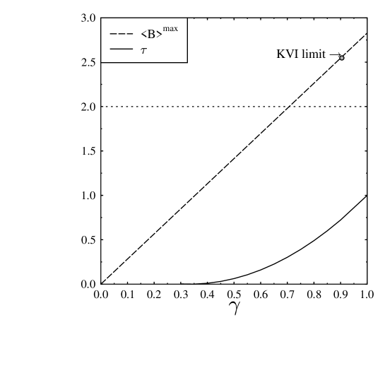
Figure 1: Plot of $\langle{\cal{B}}\rangle_{Werner}^{\max}$ (dashed line) and $\tau$ (solid line) versus the purity $\gamma$. The dotted line is the Bell limit, the circle is the KVI limit for $\gamma\sim 0.9$.

Table 1: Experimental data and quantum theory predictions for a pure singlet states (case 1) and mixed Werner states (case 2) for several violating cases of the CHSH-Bell inequality according to the definition given in Eq. 1.

CHSH-Bell	QM	QM	Exp. Data
Inequality	case 1	case 2
$E(50^{\circ},0^{\circ},25^{\circ},75^{\circ}$)	2.46	2.21	0.67$\pm$ 2.30
$E(60^{\circ},0^{\circ},30^{\circ},90^{\circ})$	2.60	2.34	1.21$\pm$ 2.42
$E(70^{\circ},0^{\circ},35^{\circ},105^{\circ})$	2.72	2.45	1.54$\pm$ 2.76
$E(80^{\circ},0^{\circ},40^{\circ},120^{\circ})$	2.80	2.52	2.11$\pm$ 2.86
$E(90^{\circ},0^{\circ},45^{\circ},135^{\circ})$	2.83	2.55	2.23$\pm$ 2.48
$E(100^{\circ},0^{\circ},50^{\circ},150^{\circ})$	2.79	2.51	2.39$\pm$ 2.87
$E(110^{\circ},0^{\circ},55^{\circ},165^{\circ})$	2.69	2.34	2.58$\pm$ 2.91
$E(120^{\circ},0^{\circ},60^{\circ},180^{\circ})$	2.50	2.25	2.75$\pm$ 2.95
$\chi^{2}$	1.26	0.85

Note that, a violation of the modified Bell-inequality does not exclude an explanation with a hidden variable theory. In Fig. 1 we plot $\langle{\cal{B}}\rangle_{Werner}^{max}$ and the tangle $\tau$ versus the purity $\gamma$. As we can see in this figure the Werner state does not violate the Bell inequality if its purity $\gamma$ is less than $1/\sqrt{2}\sim 70\verb+$. However, the entanglement is still non-zero in the Werner state until $\gamma>1/3\sim 33\verb+$. Therefore, some quantum correlation cannot be seen only by measuring the violation of the Bell-type inequality because some of them (Werner states) are entangled but still do not violate Bell inequality. Note that there is a possible experimental measurement of the entanglement based on the entanglement witness [8] that we think to implement in the future experiment.

In Tab. 1 we compare the quantum theory predictions assuming a pure singlet state (case 1) and mixed Werner states (case 2) for the spin of the two detected protons for several violating cases of the CHSH-Bell inequality. The value of $\chi^{2}=\sum_{i}({R^{i}_{th}-R^{i}_{exp}\over\Delta R^{i}_{exp}})^{2}$ is given in the bottom of the table for both cases. We have found that $\chi^{2}_{Werner}<\chi^{2}_{Singlet}$ as expected. However, we cannot judge this result as evidence of the mixing of the singlet with the unpolarized state because the experimental data suffer from large errors.

4 Conclusion

In this paper we have discussed the effect of the unpolarized state in the spin correlations measurement of the ${}^{1}S_{0}$ two proton state produced in ${\rm{{}^{12}C}}(d$,$\rm{{}^{2}He)}$ reaction at KVI. We have shown that even a small coupling (less than $10\verb+$) of the pure singlet state with the unpolarized state changes dramatically the Bell-violation value. After introducing the contribution of the unpolarized state we have found a better $\chi^{2}$. The experimental results are suffering from a large statistical error and therefore not conclusive for testing Bell’s inequality, but with a modified experimental setup, measurements with significantly improved precision will become feasible.

References

• [1] S. Hamieh and H. Zaraket,J. Phys. A: Math. Gen. 36, L387-L391 (2003).
• [2] J.S. Bell, Physics 1, 195 (1964); Rev. Mod. Phys. 38, 447 (1966).
• [3] J. Clauser, M. Horne, A. Shimony, and R. Holt,Phys. Rev. Lett. 23, 880 (1969).
• [4] R. Horodecki, P. Horodecki, and M. Horodecki, Phys. Lett. A 200, 340 (1995).
• [5] C. Polachic, C. Rangacharyulu, A. van den Berg, M. Harakeh, M. de Huu, H. Wortche, J. Heyse, C. Baumer, D. Frekers, and J. Brooke, quant-ph/0303136, submitted to Phys. Lett. A.
• [6] C. H. Bennett, D. P. DiVincenzo, J. A. Smolin and W. K. Wootters, Phys. Rev. A 54, 3824 (1996).
• [7] R.F. Werner, Phys. Rev. A 40, 4277 (1989).
• [8] O. Guhne, P. Hyllus, D. Brub, E. Ekert, M. Lewenstein, C. Macchiavello, and A. Sampera, Phys. Rev. A 66, 062305 (2002).