Analysis for practical realization of number-state manipulation
by number-sum Bell measurement with linear optics

Abstract

We analyze the linear optical realization of number-sum Bell measurement and number-state manipulation by taking into account the realistic experimental situation, specifically imperfectness of single-photon detector. The present scheme for number-state manipulation is based on the number-sum Bell measurement, which is implemented with linear optical elements, i.e., beam splitters, phase shifters and zero-one-photon detectors. Squeezed vacuum states and coherent states are used as optical sources. The linear optical Bell state detector is formulated quantum theoretically with a probability operator measure. Then, the fidelity of manipulation and preparation of number-states, particularly for qubits and qutrits, is evaluated in terms of the quantum efficiency and dark count of single-photon detector. It is found that a high fidelity is achievable with small enough squeezing parameters and coherent state amplitudes.

I Introduction

Extensive research and development have been done recently on quantum information and communication technologies. Among various media for quantum information and communication, the photon-number Fock space is promising in the point that it provides higher dimensional states such as qutrits to carry more information than qubits. This stimulates great interest in preparation and manipulation of various photon-number states. Specifically, teleportation BBCJPW ; Braunstein is known to provide important tools for quantum communication and information processing. The number-state teleportation may be performed by making a number-sum Bell measurement with certain Einstein-Podolsky-Rosen (EPR) resource BBCJPW ; Milburn . Then, its method really appears to be useful for engineering the input states, irrespective of teleportation fidelity. In fact, a quantum scissors for number-state truncation by projective measurement, which has been investigated thoroughly so far scissors1 ; scissors2 ; scissors3 , may be viewed as a teleportation-based number-state manipulation. The entanglement resource is prepared from vacuum and one photon state through a 50:50 beam splitter, and the joint photon detection implements the number-sum Bell measurement. An experimental realization of quantum scissors has been done recently, generating a qubit of vacuum and one-photon state by truncating a coherent state scissors4 . It is also interesting that an experimental result has been reported for the teleportation of the vacuum-one-photon qubit LSPM .

The number-sum Bell measurement accordingly plays an essential role for engineering the photon-number states via teleportation. Some feasible schemes have appeared recently for implementing particularly the joint measurement of number-sum and phase-difference with linear optics pdm1 ; KY-2002 ; KY-2003 ; ZPM-2003 ; ZPM-2004 , and an experimental demonstration has also been reported pdm2 . Then, various number-state preparations and manipulations have been investigated based on teleportation with number-sum Bell measurements and relevant EPR resources KY-2002 ; KY-2003 ; ZPM-2003 ; ZPM-2004 . In these respects, there are growing interests in the number-sum Bell measurement and its application for the number-state manipulation.

In this paper we analyze the linear optical realization of number-sum Bell measurement and number-state manipulation by taking into account the realistic experimental situation, specifically imperfectness of single-photon detector. The present scheme for number-state manipulation is based on the number-sum Bell measurement, which is implemented with linear optical elements, i.e., beam splitters, phase shifters and zero-one-photon detectors. As for the optical sources, many useful manipulations of number-states are realized with squeezed vacuum states and coherent states, which are widely used in optical experiments, while single-photon sources may not be required KY-2002 ; KY-2003 ; ZPM-2003 ; ZPM-2004 . Beam splitters and phase shifters will be available with high accuracy. On the other hand, photon detectors are currently developed devices, which in practice have finite quantum efficiency and nonzero dark count rate. Hence, for feasible experiments it is desired to provide a systematic method to evaluate the efficiency of number-state manipulation with number-sum Bell measurement, by taking into account the imperfectness of actual photon detectors. It is indeed encouraging that some significant developments and new proposals have been made for single-photon detection to achieve the quantum efficiency close to unity SPD1 ; SPD2 . We believe that the present work promotes future experimental efforts on engineering photon-number states by number-sum Bell measurement.

This paper is organized as follows. In Sec. II, we describe the number-sum Bell states, particularly those associated with phase-difference. In Sec. III, we present a linear optical detector to measure a specific number-sum Bell state, and formulate it quantum theoretically with a probability operator measure (POM). Then, we estimate the sensitivity of these detectors in terms of the efficiency of practical single-photon detectors. In Sec. IV, we investigate the number-state manipulation via teleportation by number-sum Bell measurement. We present the formulas to evaluate the fidelity for engineering various photon-number states. In Sec. V, by applying these formulas we analyze the efficiencies of some useful manipulations and preparations in particular for qubits and qutrits. This analysis indicates that these experiments will be performed with good fidelities by utilizing currently available apparatus. Section VI is devoted to summary.

II Number-sum Bell states

The measurement of number-sum Bell states plays the central role in the present scheme for number-state manipulation. The number-sum Bell states are given generally as

$$|{\bf d}(N,m)\rangle=\sum_{k=0}^{N}d_{k}(N,m)|N-k\rangle_{1}|k\rangle_{2}$$ (1)

for $m=0,1,\ldots,N$, forming an orthonormal set,

$$\langle{\bf d}(N^{\prime},m^{\prime})|{\bf d}(N,m)\rangle = \delta_{N^{\prime}N}{\bf d}(N,m^{\prime})\cdot{\bf d}(N,m)$$ (2)

$$= \delta_{N^{\prime}N}\delta_{m^{\prime}m}.$$

The inner product of complex vectors is henceforth represented by

$${\bf u}\cdot{\bf v}=\sum_{k=0}^{N}u_{k}^{*}v_{k}.$$ (3)

The generic states in the two-mode Fock space $\{|n_{1}\rangle_{1}|n_{2}\rangle_{2}\}$ are expanded in terms of these Bell states as

$$|\psi_{(2)}\rangle = \sum_{N=0}^{\infty}\sum_{k=0}^{N}c_{k}(N)|N-k\rangle_{1}|k\rangle_{2}$$ (4)

$$= \sum_{N=0}^{\infty}\sum_{m=0}^{N}c_{\bf d}(N,m)|{\bf d}(N,m)\rangle,$$

where

$$c_{\bf d}(N,m)={\bf d}(N,m)\cdot{\bf c}(N)=\sum_{k=0}^{N}d_{k}^{*}(N,m)c_{k}(N).$$ (5)

Specifically, we consider the number-phase Bell states L-S ; KY-2002 ; KY-2003 ; ZPM-2003 ; ZPM-2004 ,

$$|\phi_{-}(N,m)\rangle=\sum_{k=0}^{N}\frac{[(\omega_{N+1}^{*})^{m}]^{k}}{\sqrt{N+1}}|N-k\rangle_{1}|k\rangle_{2}$$ (6)

with

$$d_{k}(N,m)=\frac{1}{\sqrt{N+1}}[(\omega_{N+1}^{*})^{m}]^{k},$$ (7)

where the $(N+1)$-root to generate a ${\rm Z}_{N+1}$ is given by

$$\omega_{N+1}\equiv\exp\left[i2\pi/(N+1)\right],\ (\omega_{N+1})^{N+1}=1.$$ (8)

These Bell states in Eq. (6) are also expressed as

$$|\phi_{-}(N,m)\rangle=\sum_{m^{\prime}=0}^{N}\frac{[(\omega_{N+1}^{*})^{m^{\prime}+m}]^{N}}{\sqrt{N+1}}|\phi^{(N)}_{m^{\prime}+m}\rangle_{1}|\phi^{(N)}_{m^{\prime}}\rangle_{2}$$ (9)

in terms of the phase states given by Pegg and Barnett P-B ,

$$|\phi^{(N)}_{m}\rangle_{p}=\sum_{n=0}^{N}\frac{[(\omega_{N+1})^{m}]^{n}}{\sqrt{N+1}}|n\rangle_{p}\ (p=1,2).$$ (10)

The Bell measurement of number-sum and phase-difference is represented by the Hermitian operators,

$${\hat{N}}_{+}\equiv{\hat{N}}_{1}+{\hat{N}}_{2},$$ (11)

$${\hat{\Phi}}_{-}\equiv\sum_{N=0}^{\infty}[{\hat{\Phi}}^{(N)}_{1}-{\hat{\Phi}}^{(N)}_{2}]{\hat{P}}^{(N)}.$$ (12)

Here, ${\hat{N}}_{p}$ ($p=1,2$) represent the number operators of the respective modes, and ${\hat{\Phi}}^{(N)}_{p}$ the phase operators corresponding to the phase states in Eq. (10). The projection operator ${\hat{P}}^{(N)}$ extracts the states in the subspace $\{|N-k\rangle_{1}|k\rangle_{2}\}$ with number-sum $N$. As seen clearly from Eqs. (6) and (9), the Bell states $|\phi_{-}(N,m)\rangle$ are the simultaneous eigenstates of number-sum and phase-difference:

$${\hat{N}}_{+}|\phi_{-}(N,m)\rangle=N|\phi_{-}(N,m)\rangle,$$ (13)

$${\hat{\Phi}}_{-}|\phi_{-}(N,m)\rangle=\phi_{-}(N,m)|\phi_{-}(N,m)\rangle,$$ (14)

where the phase-difference eigenvalues are given by

$$\phi_{-}(N,m)=\frac{2\pi}{N+1}m.$$ (15)

Since $[{\hat{\Phi}}^{(N)}_{1}-{\hat{\Phi}}^{(N)}_{2}]$ does not change the number-sum $N$, it commutes with ${\hat{P}}^{(N)}$ as required for the Hermiticity of the entire phase-difference operator ${\hat{\Phi}}_{-}$. These results clarify that in the subspace with number-sum $N$ the phase-difference operator introduced by Luis and Sánchez-Soto L-S indeed coincides with the difference of the phase operators of the individual modes given by Pegg and Barnett P-B , while it is not separable in the entire two-mode Fock space. It is also obvious from Eqs. (13) and (14) that ${\hat{N}}_{+}$ and ${\hat{\Phi}}_{-}$ are commutable:

$$[{\hat{N}}_{+},{\hat{\Phi}}_{-}]=0.$$ (16)

Therefore, the joint measurement of number-sum and phase-difference can be made in principle, where the two-mode number states are projected to the number-phase Bell states $|\phi_{-}(N,m)\rangle$.

The number-phase Bell states in Eq. (6) may be generalized by introducing a scaling parameter $r$ KY-2002 ; KY-2003 as

$$|\phi_{-}(N,m,r)\rangle=D(N,r)\sum_{k=0}^{N}r^{k}[(\omega_{N+1}^{*})^{m}]^{k}|N-k\rangle_{1}|k\rangle_{2},$$ (17)

where the normalization factor is given by

$$D(N,r)=\frac{{\sqrt{N+1}}(1-r^{2})}{1-r^{2(N+1)}}.$$ (18)

A two-mode squeezed vacuum state $|\lambda\rangle$ with squeezing parameter $\lambda<1$ may be used as a primary resource of entanglement, which is given by

$$|\lambda\rangle=(1-\lambda^{2})^{1/2}\sum_{n=0}^{\infty}\lambda^{n}|n\rangle|n\rangle.$$ (19)

Then, these generalized number-phase Bell states are actually generated from a pair of two-mode squeezed vacuum states $|\lambda\rangle_{13}$ and $|\lambda^{\prime}\rangle_{24}$ by making the number-phase Bell measurement:

$$|\lambda\rangle_{13}|\lambda^{\prime}\rangle_{24}\stackrel{{\scriptstyle|\phi_{-}(N,-m)\rangle}}{{\Longrightarrow}}|\phi(N,m,r)\rangle,$$ (20)

where the scaling parameter $r$ is given by the ratio of the squeezing parameters,

$$r=\lambda^{\prime}/\lambda.$$ (21)

Here, we have considered the relation

$$|\lambda\rangle_{13}|\lambda^{\prime}\rangle_{24} = (1-\lambda^{2})^{1/2}(1-\lambda^{\prime 2})^{1/2}\sum_{N=0}^{\infty}\frac{\lambda^{N}}{D(N,r)}$$ (22)

$$\times \sum_{m=0}^{N}|\phi_{-}(N,-m)\rangle_{34}|\phi_{-}(N,m,r)\rangle_{12}$$

from the swapping $(1,3)(2,4)\rightarrow(1,2)(3,4)$.

III Practical Bell state detector

We utilize a linear optical detector, say Bell state detector, to measure conditionally a specific two-mode number-sum Bell state as given in Eq. (1). Henceforth the Bell state to be detected is denoted simply by

$$|{\tilde{\bf d}}\rangle\equiv|{\bf d}({\tilde{N}},{\tilde{m}})\rangle$$ (23)

with the number-sum ${\tilde{N}}$ and amplitude coefficients

$${\tilde{d}}_{k}\equiv d_{k}({\tilde{N}},{\tilde{m}}).$$ (24)

As shown schematically in Fig. 1, it is constructed as an $M$-port system consisting of (i) a set of beam splitters and phase shifters, (ii) $(M-2)$ auxiliary input modes (ancillas) with vacuum states, and (iii) zero-one-resolving photon detectors for the output modes, though imperfect practically. This method is based on the idea of photon chopping chopping . The Bell state detectors of $|\phi_{-}({\tilde{N}},{\tilde{m}})\rangle$ for ${\tilde{N}}=1$ and $2$ are considered in Refs. KY-2002 ; KY-2003 , and then a method for general ${\tilde{N}}$ is presented in Refs. ZPM-2003 ; ZPM-2004 . The photon detectors need to resolve zero, one or more photons, since two or more photons may enter some of the detectors for the case of ${\tilde{N}}\geq 2$.

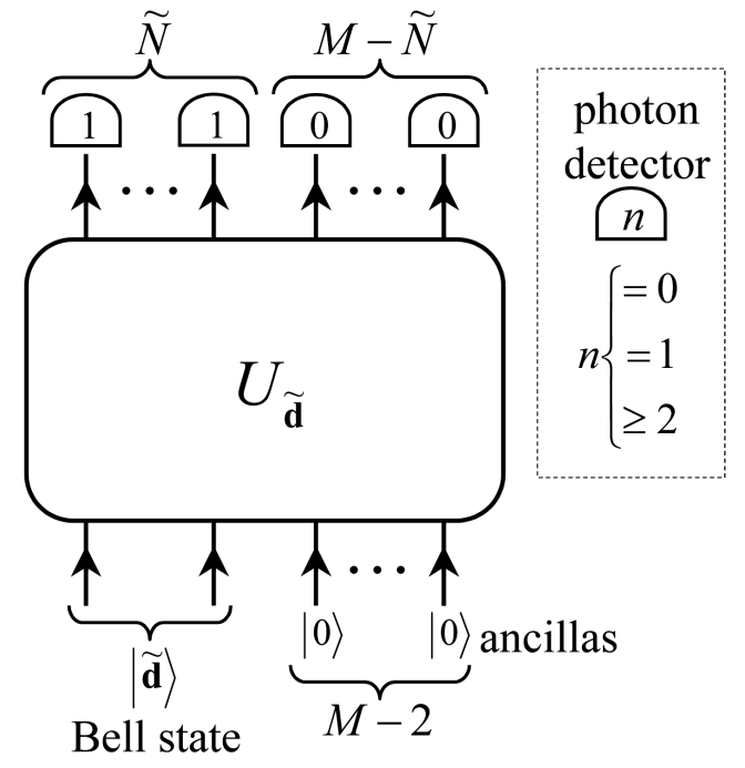
Figure 1: A schematic diagram of the linear optical Bell state detector. The input two-mode state, which may contain the number-sum Bell state $|{\tilde{\bf d}}\rangle\equiv|{\bf d}({\tilde{N}},{\tilde{m}})\rangle$ with number-sum ${\tilde{N}}$, enters the detector together with the vacuum states of $(M-2)$ ancilla modes. A unitary transformation $U_{\tilde{\bf d}}$ is made through a set of beam splitters and phase shifters, and the output state is detected to give conditionally the specific photon count ${\bf n}_{(M)}^{\rm cnt}=(1,\ldots,1,0,\ldots,0)$ as the signal of $|{\tilde{\bf d}}\rangle$. The photon detectors need to resolve zero, one or more photons, since two or more photons may enter some of the detectors for the case of ${\tilde{N}}\geq 2$.

The operation of the set of beam splitters and phase shifters is given by a unitary transformation between the input modes $a_{i}$ and the output modes $b_{j}$ (in Heisenberg picture) Reck-Zeilinger :

$$a_{i}={\cal U}_{\tilde{\bf d}}b_{i}{\cal U}_{\tilde{\bf d}}^{\dagger}=U_{\tilde{\bf d}ij}b_{j},\ a_{i}^{\dagger}={\cal U}_{\tilde{\bf d}}b_{i}^{\dagger}{\cal U}_{\tilde{\bf d}}^{\dagger}=b_{j}^{\dagger}U_{\tilde{\bf d}ji}^{\dagger},$$ (25)

where $i,j=1,2,\ldots,M$, and $U_{\tilde{\bf d}}$ is an $M\times M$ unitary matrix. The two-mode input state $|\psi_{(2)}\rangle$ and vacuum state $|{\bf 0}\rangle_{\bf a}$ of $(M-2)$ ancillas are transformed to certain output state through the optical set (in Schrödinger picture), which may be expanded in terms of the number-states of the output $M$ modes,

$$|{\bf n}_{(M)}\rangle\equiv|n_{1}\rangle_{1}|n_{2}\rangle_{2}\cdots|n_{M}\rangle_{M}$$ (26)

with number distribution

$${\bf n}_{(M)}\equiv(n_{1},n_{2},\ldots,n_{M}).$$ (27)

The parameters of the optical set are chosen so that this unitary transformation is given as

$${\cal U}_{\tilde{\bf d}}|\psi_{(2)}\rangle|{\bf 0}\rangle_{\bf a}=g_{\tilde{\bf d}}\langle{\tilde{\bf d}}|\psi_{(2)}\rangle|{\bf n}_{(M)}^{\rm cnt}\rangle+|\Psi\bot{\bf n}_{(M)}^{\rm cnt}\rangle,$$ (28)

where $|\Psi\bot{\bf n}_{(M)}^{\rm cnt}\rangle$ is a certain state orthogonal to $|{\bf n}_{(M)}^{\rm cnt}\rangle$. That is, only if the input state $|\psi_{(2)}\rangle$ contains the Bell state $|{\tilde{\bf d}}\rangle$ to be detected, the output state has the component of the specific number distribution,

$${\bf n}_{(M)}^{\rm cnt}=(\overbrace{1,\ldots,1}^{\tilde{N}},\overbrace{0,\ldots,0}^{M-{\tilde{N}}}).$$ (29)

Then, by using the ideal zero-one-resolving photon detectors, the Bell state $|{\tilde{\bf d}}\rangle$ is detected conditionally in $|\psi_{(2)}\rangle$, when the photon counting result of ${\bf n}_{(M)}^{\rm cnt}$ is obtained with success probability

$$P_{\tilde{\bf d}}^{\rm ideal}[|\psi_{(2)}\rangle]=|g_{\tilde{\bf d}}|^{2}|\langle{\tilde{\bf d}}|\psi_{(2)}\rangle|^{2}.$$ (30)

Practically, we use imperfect zero-one-resolving photon detectors described by the POM’s $\Pi(0)$ and $\Pi(1)$. The POM of photon detector for the $N$ photon count is given with quantum efficiency $\eta$ and mean dark count $\nu$ by

$$\Pi(N) = \sum_{m=0}^{N}{\rm e}^{-\nu}\frac{\nu^{N-m}}{(N-m)!}$$ (31)

$$\times \sum_{n=m}^{\infty}{}_{n}C_{m}\eta^{m}(1-\eta)^{n-m}|n\rangle\langle n|,$$

where ${}_{n}C_{m}$ is the binomial coefficient Barnett-Phillips-Pegg .

The two-mode input state $\rho_{(2)}$ combined with the ancilla-mode $\rho_{\bf a}$ is transformed by the optical set as

$$\rho_{(2)}\otimes\rho_{\bf a}\rightarrow{\cal U}_{\tilde{\bf d}}\rho_{(2)}\otimes\rho_{\bf a}{\cal U}_{\tilde{\bf d}}^{\dagger},$$ (32)

where

$$\rho_{\bf a}=|{\bf 0}\rangle_{\bf a}{}_{\bf a}\langle{\bf 0}|\equiv\mathop{\otimes}_{i=3}^{M}(|0\rangle\langle 0|)_{i}.$$ (33)

Then, the probability to obtain the photon count of Eq. (29) for the two-mode $\rho_{(2)}$ is given by

$$P_{\tilde{\bf d}}[\rho_{(2)}] = {\rm Tr}[\Pi_{\rm PD}{\cal U}_{\tilde{\bf d}}\rho_{(2)}\otimes\rho_{\bf a}{\cal U}_{\tilde{\bf d}}^{\dagger}]$$ (34)

$$\equiv {\rm Tr}[\Gamma_{\tilde{\bf d}}\rho_{(2)}].$$

The POM of this Bell state detector is given by

$$\Gamma_{\tilde{\bf d}}={}_{\bf a}\langle{\bf 0}|{\cal U}_{\tilde{\bf d}}^{\dagger}\Pi_{\rm PD}{\cal U}_{\tilde{\bf d}}|{\bf 0}\rangle_{\bf a}$$ (35)

with the POM of the photon detector set

$$\Pi_{\rm PD}=\mathop{\otimes}_{i=1}^{\tilde{N}}\Pi(1)_{i}\mathop{\otimes}_{i={\tilde{N}}+1}^{M}\Pi(0)_{i}.$$ (36)

It may be expressed as

$$\Gamma_{\tilde{\bf d}}=\sum_{N=0}^{\infty}\sum_{k=0}^{N}\sum_{k^{\prime}=0}^{N}K^{\tilde{\bf d}}_{k^{\prime}k}(N)|(N,k^{\prime})\rangle\langle(N,k)|$$ (37)

in terms of the basis states of number-sum $N$

$$|(N,k)\rangle\equiv|N-k\rangle_{1}|k\rangle_{2}$$ (38)

with

$$K^{\tilde{\bf d}}_{k^{\prime}k}(N)\delta_{N^{\prime}N}=\langle(N^{\prime},k^{\prime})|\Gamma_{\tilde{\bf d}}|(N,k)\rangle.$$ (39)

Here, it should be remarked that the matrix elements of $\Gamma_{\tilde{\bf d}}$ between the states with different values of number-sum are zero, since ${\cal U}_{\tilde{\bf d}}$ and $\Pi_{\rm PD}$ conserve the total photon number.

Specifically, for the basis state $|(N,k)\rangle$ we obtain the output state as

$${\cal U}_{\tilde{\bf d}}|(N,k)\rangle|{\bf 0}\rangle_{\bf a}=\sum_{N_{\Sigma}[{\bf n}_{(M)}]=N}B^{\tilde{\bf d}}_{k}[{\bf n}_{(M)}]|{\bf n}_{(M)}\rangle.$$ (40)

Here, the sum is taken over the distributions ${\bf n}_{(M)}$ with number-sum $N$, since the unitary transformation ${\cal U}_{\tilde{\bf d}}$ conserves the total photon number

$$N_{\Sigma}[{\bf n}_{(M)}]\equiv\sum_{i=1}^{M}n_{i}=N.$$ (41)

The basis states with number-sum $N$ are given by

$$|(N,k)\rangle=\frac{1}{{\sqrt{(N-k)!}}{\sqrt{k!}}}(a_{1}^{\dagger})^{N-k}(a_{2}^{\dagger})^{k}|0\rangle_{1}|0\rangle_{2}.$$ (42)

By using Eq. (25) we obtain

$$(a_{1}^{\dagger})^{N-k}(a_{2}^{\dagger})^{k}=\sum_{{\bf j}_{(N)}}W^{\tilde{\bf d}}_{k}[{\bf j}_{(N)}]\mathop{\otimes}_{l=1}^{N}b_{j_{l}}^{\dagger},$$ (43)

where ${\bf j}_{(N)}\equiv(j_{1},j_{2},\ldots,j_{N})$, $1\leq j_{l}\leq M$, and

$$W^{\tilde{\bf d}}_{k}[{{\bf j}_{(N)}}]=U_{{\tilde{\bf d}}1j_{1}}^{*}\cdots U_{{\tilde{\bf d}}1j_{N-k}}^{*}U_{{\tilde{\bf d}}2j_{N-k+1}}^{*}\cdots U_{{\tilde{\bf d}}2j_{N}}^{*}.$$ (44)

Then, we calculate the coefficients for the output state $|{\bf n}_{(M)}\rangle$ in Eq. (40) as

$$B^{\tilde{\bf d}}_{k}[{\bf n}_{(M)}]=\frac{\sqrt{{\bf n}_{(M)}!}}{{\sqrt{(N-k)!}}{\sqrt{k!}}}\sum_{{\bf j}_{(N)}\to{\bf n}_{(M)}}W^{\tilde{\bf d}}_{k}[{\bf j}_{(N)}],$$ (45)

where ${\bf n}_{(M)}!\equiv n_{1}!n_{2}!\cdots n_{M}!$, and the sum is taken over all the sets of indices ${\bf j}_{(N)}$ that provide the photon-number distribution ${\bf n}_{(M)}$.

Given the the coefficients $B^{\tilde{\bf d}}_{k}[{\bf n}_{(M)}]$ in Eq. (40), we obtain the matrix elements of Bell measurement POM $\Gamma_{\tilde{\bf d}}$ in Eq. (37) as

$$K^{\tilde{\bf d}}_{k^{\prime}k}(N)=\sum_{N_{\Sigma}[{\bf n}_{(M)}]=N}B^{{\tilde{\bf d}}*}_{k^{\prime}}[{\bf n}_{(M)}]B^{\tilde{\bf d}}_{k}[{\bf n}_{(M)}]P_{\rm PD}[|{\bf n}_{(M)}\rangle].$$ (46)

Here, we have considered the relation from the photon-number conserving nature of $\Pi_{\rm PD}$,

$$\langle{\bf n}_{(M)}^{\prime}|\Pi_{\rm PD}|{\bf n}_{(M)}\rangle=\delta_{{\bf n}_{(M)}^{\prime}{\bf n}_{(M)}}P_{\rm PD}[|{\bf n}_{(M)}\rangle].$$ (47)

The probability that the state $|{\bf n}_{(M)}\rangle$ results in the photon count ${\bf n}_{(M)}^{\rm cnt}$ is given by

$$P_{\rm PD}[|{\bf n}_{(M)}\rangle] = \langle{\bf n}_{(M)}|\Pi_{\rm PD}|{\bf n}_{(M)}\rangle$$ (48)

$$= \prod_{i=1}^{\tilde{N}}P_{1\gamma}(n_{i})\prod_{i={\tilde{N}}+1}^{M}P_{0\gamma}(n_{i}),$$

where

$$P_{0\gamma}(n)=\langle n|\Pi(0)|n\rangle={\rm e}^{-\nu}{\delta\eta}^{n},$$ (49)

$$P_{1\gamma}(n)=\langle n|\Pi(1)|n\rangle={\rm e}^{-\nu}{\delta\eta}^{n-1}[n(1-{\delta\eta})+\nu{\delta\eta}]$$

with

$$\delta\eta\equiv 1-\eta.$$ (51)

The output state $|{\bf n}_{(M)}^{\rm cnt}\rangle$, in particular, to indicate the desired Bell state $|{\tilde{\bf d}}\rangle$ is faithfully counted as ${\bf n}_{(M)}^{\rm cnt}$ with probability

$$P_{\rm PD}[|{\bf n}_{(M)}^{\rm cnt}\rangle]={\rm e}^{-M\nu}[1-{\delta\eta}+\nu{\delta\eta}]^{\tilde{N}}.$$ (52)

(Henceforth we assume for simplicity that all the photon detectors have the common $\eta$ and $\nu$.) The probability for the generic output state $|{\bf n}_{(M)}\rangle$ to give the expected photon count ${\bf n}_{(M)}^{\rm cnt}$ is also evaluated as

$$P_{\rm PD}[|{\bf n}_{(M)}\rangle]={\rm e}^{-M\nu}\sum_{(a,b)}r_{\rm PD}^{(a,b)}[{\bf n}_{(M)}]{\delta\eta}^{a}\nu^{b}(1-{\delta\eta})^{{\tilde{N}}-b}$$ (53)

with certain coefficients $r_{\rm PD}^{(a,b)}[{\bf n}_{(M)}]$, where the extra factors $(1-{\delta\eta})^{{\tilde{N}}-b}$ come from $P_{1\gamma}(n_{i})$ ($1\leq i\leq{\tilde{N}}$). The non-negative powers $a$ and $b$ in the expansion of Eq. (53) represent the discounts and overcounts of photons, respectively, which satisfy the relation

$$a-b=N-{\tilde{N}}$$ (54)

in the range of ${\rm max}[0,N-{\tilde{N}}]\leq a\leq N$ and ${\rm max}[0,{\tilde{N}}-N]\leq b\leq{\tilde{N}}$. For $N<{\tilde{N}}$ the deficit of photons should be supplied by the dark counts, while for $N>{\tilde{N}}$ the excess of photons should be discarded with $\eta<1$. By considering Eq. (54), the leading dependence of $P_{\rm PD}[|{\bf n}_{(M)}\rangle]$ on ${\delta\eta}<1$ and $\nu<1$ is found for the output states other than $|{\bf n}_{(M)}^{\rm cnt}\rangle$ as

$$P_{\rm PD}[|{\bf n}_{(M)}\rangle\not=|{\bf n}_{(M)}^{\rm cnt}\rangle]\sim\left\{\begin{array}[]{ll}\nu^{{\tilde{N}}-N}&(N<{\tilde{N}})\\ {\delta\eta}\nu&(N={\tilde{N}})\\ {\delta\eta}^{N-{\tilde{N}}}&(N>{\tilde{N}})\end{array}\right..$$ (55)

It may be reasonably assumed for feasible photon detectors that the dark count $\nu$ is considerably smaller than the inefficiency ${\delta\eta}$, e.g., $\nu\sim 10^{-4}$ and ${\delta\eta}\sim 0.1$, as will be explained in Sec. V. Then, the leading error $\sim{\delta\eta}$ of the Bell state detector is provided by the states $|{\bf n}_{(M)}\rangle$ with the total photon number $N={\tilde{N}}+1$.

When the desired Bell state $|{\tilde{\bf d}}\rangle$ is measured by this Bell state detector, the probability to obtain the expected photon count ${\bf n}_{(M)}^{\rm cnt}$ is given with Eqs. (34), (37) and (46) as

$$P_{\tilde{\bf d}}[|{\tilde{\bf d}}\rangle] = {\rm Tr}[\Gamma_{\tilde{\bf d}}|{\tilde{\bf d}}\rangle\langle{\tilde{\bf d}}|]$$

$$= \sum_{N_{\Sigma}[{\bf n}_{(M)}]={\tilde{N}}}P_{\rm PD}[|{\bf n}_{(M)}\rangle]\left|{\bf B}^{\tilde{\bf d}}[{\bf n}_{(M)}]\cdot{\tilde{\bf d}}\right|^{2}.$$

In this practical Bell measurement, the other states orthogonal to $|{\tilde{\bf d}}\rangle$ may be miscounted as $|{\tilde{\bf d}}\rangle$ with nonzero probabilities. Only if we can use the ideal Bell state detector, the Bell state is measured faithfully as

$$P_{\tilde{\bf d}}^{\rm ideal}[|{\bf d}(N,m)\rangle]={\bar{P}}_{\tilde{\bf d}}[|{\tilde{\bf d}}\rangle]\delta_{N{\tilde{N}}}\delta_{m{\tilde{m}}}.$$ (57)

That is, the desired Bell state $|{\tilde{\bf d}}\rangle$ is measured with the success probability ${\bar{P}}_{\tilde{\bf d}}[|{\tilde{\bf d}}\rangle]$, while the other orthogonal states are not detected. By considering Eq. (28) with $P_{\rm PD}^{\rm ideal}[|{\bf n}_{(M)}^{\rm cnt}\rangle]=1$, the success probability in the ideal case is evaluated as

$${\bar{P}}_{\tilde{\bf d}}[|{\tilde{\bf d}}\rangle]=|g_{\tilde{\bf d}}|^{2}=\left|{\bf B}^{\tilde{\bf d}}[{\bf n}_{(M)}^{\rm cnt}]\cdot{\tilde{\bf d}}\right|^{2}.$$ (58)

On the other hand, from the completeness of number-state Fock space the sum of the probabilities for the orthonormal basis states $|{\bf d}(N,m)\rangle\equiv|{\tilde{\bf d}}_{\bot}\rangle$ other than $|{\tilde{\bf d}}\rangle$ to be miscounted as $|{\tilde{\bf d}}\rangle$ is given by

$$\sum_{|{\tilde{\bf d}}_{\bot}\rangle}{\rm Tr}[\Gamma_{\tilde{\bf d}}[|{\tilde{\bf d}}_{\bot}\rangle\langle{\tilde{\bf d}}_{\bot}|]={\rm Tr}[\Gamma_{\tilde{\bf d}}]-{\rm Tr}[\Gamma_{\tilde{\bf d}}[|{\tilde{\bf d}}\rangle\langle{\tilde{\bf d}}|],$$ (59)

where

$${\bf 1} = |{\tilde{\bf d}}\rangle\langle{\tilde{\bf d}}|+\sum_{|{\tilde{\bf d}}_{\bot}\rangle}|{\tilde{\bf d}}_{\bot}\rangle\langle{\tilde{\bf d}}_{\bot}|,$$ (60)

$${\rm Tr}[\Gamma_{\tilde{\bf d}}] = \sum_{{\bf n}_{(M)}}P_{\rm PD}[|{\bf n}_{(M)}\rangle]\left|{\bf B}^{\tilde{\bf d}}[{\bf n}_{(M)}]\right|^{2}.$$ (61)

Then, the confidence of this practical Bell state detector may be defined by

$${\cal C}_{\tilde{\bf d}} = \frac{{\rm Tr}[\Gamma_{\tilde{\bf d}}|{\tilde{\bf d}}\rangle\langle{\tilde{\bf d}}|]}{{\rm Tr}[\Gamma_{\tilde{\bf d}}]}\leq 1.$$ (62)

In particular, ${\cal C}_{\tilde{\bf d}}=1$ only for the Bell state detector with ideal optical devices. We evaluate the confidence in Eq. (62) with Eqs. (LABEL:P-Bell) and (61) for the practical Bell state detector as

$${\cal C}_{\tilde{\bf d}} \equiv 1-\Delta{\cal C}_{\tilde{\bf d}}$$ (63)

$$= 1-\sum_{(a,b)\not=(0,0)}q_{\tilde{\bf d}}^{(a,b)}{\delta\eta}^{a}\nu^{b}$$

in the expansion with respect to $\delta\eta$ and $\nu$.

IV Number-state manipulation

We now investigate the number-state manipulation via teleportation with number-sum Bell measurement. The input state (normalized) may be prepared in $K$ optical modes as

$$|\psi_{\rm in}\rangle=\sum_{{\bf n}_{(K)}}c^{\rm in}_{{\bf n}_{(K)}}|{{\bf n}_{(K)}}\rangle,$$ (64)

where

$$|{{\bf n}_{(K)}}\rangle\equiv|n_{1}\rangle_{1}|n_{2}\rangle_{2}\cdots|n_{K}\rangle_{K}\equiv|n_{1}\rangle_{1}|{{\bf n}_{(K-1)}}\rangle.$$ (65)

We here consider specifically a class of two-mode EPR resources (normalized) as

$$|{\rm EPR}\rangle=\sum_{l=0}^{\infty}E_{l}|l\rangle_{0}|s(l)\rangle_{-1}\equiv\sum_{l=0}^{\infty}\sum_{l^{\prime}=0}^{\infty}E_{l^{\prime}l}|l\rangle_{0}|l^{\prime}\rangle_{-1}$$ (66)

with the amplitude distribution matrix

$$E_{l^{\prime}l}=\delta_{l^{\prime}s(l)}E_{l}.$$ (67)

The permutation of number-states between the two modes is given by

$$s(l_{1})\not=s(l_{2})\leftrightarrow l_{1}\not=l_{2}.$$ (68)

In particular, for the number-difference 0 resource and the number-sum $N$ resource, respectively,

$$s(l)=\left\{\begin{array}[]{ll}l&({\mbox{number-difference 0}})\\ N-l&({\mbox{number-sum $N$}})\end{array}\right..$$ (69)

The input state is then manipulated by making a Bell measurement with an EPR resource. We here consider the one-mode manipulation with the measurement of $|{\tilde{\bf d}}\rangle$. The multimode manipulation may further be performed by applying these sorts of one-mode manipulations to some modes of the input state.

The Bell measurement is made on the 0-1 mode of the combined state ($n_{1}\equiv k$, $l\equiv N-k$)

$$|\psi_{\rm in}\rangle|{\rm EPR}\rangle = \sum_{{\bf n}_{(K-1)}}\sum_{N=0}^{\infty}\sum_{k=0}^{N}c^{\rm in}_{k{\bf n}_{(K-1)}}E_{N-k}|(N,k)\rangle$$ (70)

$$\times |s(N-k)\rangle_{-1}|{{\bf n}_{(K-1)}}\rangle.$$

Then, we obtain the output state as

$$\rho_{\rm out} = {\rm Tr}[\Gamma_{\tilde{\bf d}}\rho_{\rm in}\otimes\rho_{\rm EPR}]$$

$$= \sum_{{\bf n}_{(M)}}P_{\rm PD}[|{\bf n}_{(M)}\rangle]|\psi_{\rm out}[{\bf n}_{(M)}]\rangle\langle\psi_{\rm out}[{\bf n}_{(M)}]|$$

for $\rho_{\rm in}=|\psi_{\rm in}\rangle\langle\psi_{\rm in}|$ and $\rho_{\rm EPR}=|{\rm EPR}\rangle\langle{\rm EPR}|$, where $|s(N-k)\rangle_{-1}|{{\bf n}_{(K-1)}}\rangle\equiv|{\bf n}_{(K)}\rangle$ by redenoting

$$|s(N-k)\rangle_{-1}\equiv|n_{1}\rangle_{1}.$$ (72)

(The output state $\rho_{\rm out}$ will be properly normalized later in defining the fidelity.) The output states associated with $|{\bf n}_{(M)}\rangle$, which may not be orthogonal each other, are given by

$$|\psi_{\rm out}[{\bf n}_{(M)}]\rangle=\sum_{{\bf n}_{(K)}}c^{\rm out}_{{\bf n}_{(K)}}[{{\bf n}_{(M)}}]|{\bf n}_{(K)}\rangle$$ (73)

with the amplitudes

$$c^{\rm out}_{{\bf n}_{(K)}}[{\bf n}_{(M)}]=\left.E_{N-k}B^{\tilde{\bf d}}_{k}[{\bf n}_{(M)}]c^{\rm in}_{k{\bf n}_{(K-1)}}\right|^{N=N_{\Sigma}[{\bf n}_{(M)}]}_{n_{1}=s(N-k)},$$ (74)

where $k$ is specified by $n_{1}=s(N-k)$ in terms of $n_{1}$ and $N$. It is straightforward to extend these formulas generally for the mixed states of $\rho_{\rm in}$ and $\rho_{\rm EPR}$ with the output states as $|\psi_{\rm out}[{\bf n}_{(M)}]\rangle\langle\psi_{\rm out}[{\bf n}_{(M)}]|\rightarrow\rho_{\rm out}[{\bf n}_{(M)}]$.

This teleportation-based manipulation may be viewed as a linear transformation of the input state:

$$\rho_{\rm out} = {\cal T}_{{\tilde{\bf d}}{\bf E}}\rho_{\rm in}{\cal T}_{{\tilde{\bf d}}{\bf E}}^{\dagger}$$

$$\equiv \sum_{{\bf n}_{(M)}}P_{\rm PD}[|{\bf n}_{(M)}\rangle]\left({\cal T}_{{\tilde{\bf d}}{\bf E}}[{\bf n}_{(M)}]\rho_{\rm in}{\cal T}_{{\tilde{\bf d}}{\bf E}}^{\dagger}[{\bf n}_{(M)}]\right).$$

The amplitudes are accordingly transformed as

$${\bf c}^{\rm out}[{\bf n}_{(M)}]={\bf T}^{{\tilde{\bf d}}{\bf E}}[{\bf n}_{(M)}]{\bf c}^{\rm in}$$ (76)

or

$$c^{\rm out}_{{\bf n}_{(K)}}[{\bf n}_{(M)}]=\sum_{k=0}^{N}T^{{\tilde{\bf d}}{\bf E}}_{n_{1}k}[{\bf n}_{(M)}]c^{\rm in}_{k{\bf n}_{(K-1)}}.$$ (77)

As seen from Eq. (74), the transformation matrix ${\bf T}^{{\tilde{\bf d}}{\bf E}}[{\bf n}_{(M)}]$ is composed of that given by the Bell state detector, ${\bf B}^{\tilde{\bf d}}[{\bf n}_{(M)}]$, the reversal ($0,\ldots,N\rightarrow N,\ldots,0$) with $N=N_{\Sigma}[{\bf n}_{(M)}]$, ${\bf R}_{N}$, and the EPR resource, ${\bf E}$:

$${\bf T}^{{\tilde{\bf d}}{\bf E}}[{\bf n}_{(M)}]={\bf E}{\bf R}_{N}{\bf B}^{\tilde{\bf d}}[{\bf n}_{(M)}],$$ (78)

where

$$({\bf B}^{\tilde{\bf d}}[{\bf n}_{(M)}])_{kk^{\prime}}=\delta_{kk^{\prime}}B^{\tilde{\bf d}}_{k}[{\bf n}_{(M)}]\theta(N-k)$$ (79)

with

$$\theta(N-k)=\left\{\begin{array}[]{ll}1&(0\leq k\leq N)\\ 0&(k>N)\end{array}\right..$$ (80)

We may further consider multiple of manipulations of this sort KY-2003 as

$${\cal T}^{{\tilde{\bf d}}{\bf E}(L)}\cdots{\cal T}^{{\tilde{\bf d}}{\bf E}(2)}{\cal T}^{{\tilde{\bf d}}{\bf E}(1)}.$$ (81)

The desired manipulation of input state with the EPR resource is obtained by using the ideal Bell state detector of $|{\tilde{\bf d}}\rangle$ as

$$\rho_{\rm out}(\eta=1,\nu=0)=|\psi_{\rm out}^{{\tilde{\bf d}}{\bf E}}\rangle\langle\psi_{\rm out}^{{\tilde{\bf d}}{\bf E}}|,$$ (82)

where

$$|\psi_{\rm out}^{{\tilde{\bf d}}{\bf E}}\rangle=|\psi_{\rm out}[{\bf n}_{(M)}={\bf n}_{(M)}^{\rm cnt}]\rangle$$ (83)

with

$$c^{\rm out}_{{\bf n}_{(K)}}[{\bf n}_{(M)}^{\rm cnt}]=\sum_{k=0}^{N}T^{{\tilde{\bf d}}{\bf E}}_{n_{1}k}[{\bf n}_{(M)}^{\rm cnt}]c^{\rm in}_{k{\bf n}_{(K-1)}}.$$ (84)

Here, only the number-state $|{\bf n}_{(M)}^{\rm cnt}\rangle$ is detected faithfully as the photon count ${\bf n}_{(M)}^{\rm cnt}$ in the output $M$ ports. The fidelity is used to evaluate the quality of manipulation with the practical experimental setup, which is given by

$$F[|\psi_{\rm out}^{{\tilde{\bf d}}{\bf E}}\rangle]=\frac{{\rm Tr}[\rho_{\rm out}|\psi_{\rm out}^{{\tilde{\bf d}}{\bf E}}\rangle\langle\psi_{\rm out}^{{\tilde{\bf d}}{\bf E}}|]}{{\rm Tr}[\rho_{\rm out}]{\rm Tr}[|\psi_{\rm out}^{{\tilde{\bf d}}{\bf E}}\rangle\langle\psi_{\rm out}^{{\tilde{\bf d}}{\bf E}}|]}\leq 1,$$ (85)

where the denominator of the right side provides the normalization factors of $\rho_{\rm out}$ and $|\psi_{\rm out}^{{\tilde{\bf d}}{\bf E}}\rangle\langle\psi_{\rm out}^{{\tilde{\bf d}}{\bf E}}|$. The relevant quantities are calculated by

$${\rm Tr}[\rho_{\rm out}] = \sum_{{\bf n}_{(M)}}P_{\rm PD}[|{\bf n}_{(M)}\rangle]$$ (86)

$$\times {\bf c}^{\rm out}[{\bf n}_{(M)}]\cdot{\bf c}^{\rm out}[{\bf n}_{(M)}],$$

$${\rm Tr}[|\psi_{\rm out}^{{\tilde{\bf d}}{\bf E}}\rangle\langle\psi_{\rm out}^{{\tilde{\bf d}}{\bf E}}|] = {\bf c}^{\rm out}[{\bf n}_{(M)}^{\rm cnt}]\cdot{\bf c}^{\rm out}[{\bf n}_{(M)}^{\rm cnt}],$$ (87)

$${\rm Tr}[\rho_{\rm out}|\psi_{\rm out}^{{\tilde{\bf d}}{\bf E}}\rangle\langle\psi_{\rm out}^{{\tilde{\bf d}}{\bf E}}|] = \sum_{{\bf n}_{(M)}}P_{\rm PD}[|{\bf n}_{(M)}\rangle]$$ (88)

$$\times \left|{\bf c}^{\rm out}[{\bf n}_{(M)}]\cdot{\bf c}^{\rm out}[{\bf n}_{(M)}^{\rm cnt}]\right|^{2}.\ \ \$$

Here, ${\rm Tr}[\rho_{\rm out}]$ is the probability to obtain the expected photon count ${\bf n}_{(M)}^{\rm cnt}$ by performing the conditional measurement with this Bell state detector. The fidelity of manipulation is then evaluated by considering the sensitivity of photon detector as

$$F[|\psi_{\rm out}^{{\tilde{\bf d}}{\bf E}}\rangle] \equiv 1-\Delta F[|\psi_{\rm out}^{{\tilde{\bf d}}{\bf E}}\rangle]$$ (89)

$$= 1-\sum_{(a,b)\not=(0,0)}f^{(a,b)}[|\psi_{\rm out}^{{\tilde{\bf d}}{\bf E}}\rangle]{\delta\eta}^{a}\nu^{b}.$$

V Analysis of efficiencies

We can analyze the efficiencies of practical Bell state detectors and number-state manipulations by applying the formulas presented so far.

V.1 Bell state detectors

In the number-state manipulations based on teleportation, the number-phase Bell states $|\phi_{-}(N,m)\rangle$ in Eq. (6) may specifically be measured by the Bell state detectors KY-2002 ; KY-2003 ; ZPM-2003 ; ZPM-2004 . In order to show the efficiency of practical Bell measurement with linear optics in the present scheme, we evaluate the confidence typically for the detection of $|{\tilde{\bf d}}\rangle=|\phi_{-}({\tilde{N}},0)\rangle$ with number-sum ${\tilde{N}}=1,2$ and phase-difference $m=0$. The number-phase Bell states with nonzero phase-difference $m$ are also measured similarly by making a phase shift $a_{2}\rightarrow\omega_{{\tilde{N}}+1}^{m}a_{2}$ of the mode 2 in Eq. (6) before the two-mode states enter the Bell state detector. The Bell state detectors for number-sum ${\tilde{N}}=1,2$ are useful for manipulations of qubits and qutrits, as seen later.

The Bell state detector of $|\phi_{-}(1,0)\rangle$ with ${\tilde{N}}=1$ is characterized by the amplitude distribution and the unitary transformation of optical modes which are given, respectively, by

$${\tilde{\bf d}} = \frac{1}{\sqrt{2}}\left(\begin{array}[]{c}1\\ 1\end{array}\right)\rightarrow|\phi_{-}({\tilde{N}}=1,0)\rangle,$$ (92)

$$U_{\tilde{\bf d}} = \left(\begin{array}[]{cc}\frac{1}{\sqrt{2}}&-\frac{1}{\sqrt{2}}\\ \frac{1}{\sqrt{2}}&\frac{1}{\sqrt{2}}\end{array}\right),$$ (95)

where no ancilla is used ($M=2$). As is well-known, this unitary transformation $U_{\tilde{\bf d}}$ is realized with a 50:50 beam splitter. The confidence of this Bell state detector is calculated in the leading orders of the expansion with respect to $\delta\eta$ and $\nu$ as

$$\Delta{\cal C}_{\tilde{\bf d}}\equiv 1-{\cal C}_{\tilde{\bf d}}[|\phi_{-}({\tilde{N}}=1,0)\rangle]:$$

$$\left[\begin{array}[]{ccc}a&q_{\tilde{\bf d}}^{(a,0)}{\delta\eta}^{a}&q_{\tilde{\bf d}}^{(a,1)}\nu{\delta\eta}^{a}\\ 0&-\!\!\!-\!\!\!-&1\\ 1&3&-4\\ 2&-3&5\\ 3&1&-2\\ 4&0&0\end{array}\right]\ ,$$ (102)

where the coefficients $q_{\tilde{\bf d}}^{(a,b)}$ are presented in this list. The Bell state detector of $|\phi_{-}(2,0)\rangle$ with ${\tilde{N}}=2$ is characterized by

$${\tilde{\bf d}} = \frac{1}{\sqrt{3}}\left(\begin{array}[]{c}1\\ 1\\ 1\end{array}\right)\rightarrow|\phi_{-}({\tilde{N}}=2,0)\rangle,$$ (106)

$$U_{\tilde{\bf d}} = \left(\begin{array}[]{ccc}\frac{1}{\sqrt{2}}&0&-\frac{1}{\sqrt{2}}\\ 0&1&0\\ \frac{1}{\sqrt{2}}&0&\frac{1}{\sqrt{2}}\end{array}\right)\left(\begin{array}[]{ccc}1&0&0\\ 0&\frac{2}{\sqrt{6}}&-\frac{1}{\sqrt{3}}\\ 0&\frac{1+i}{\sqrt{6}}&\frac{1+i}{\sqrt{3}}\end{array}\right)$$ (117)

$$\times\left(\begin{array}[]{ccc}1&0&0\\ 0&\frac{{\sqrt{3}}(3+i)}{4{\sqrt{5}}}&-\frac{3+i}{4}\\ 0&\frac{\sqrt{5}}{2{\sqrt{2}}}&\frac{\sqrt{3}}{2{\sqrt{2}}}\end{array}\right),$$

where one ancilla is used ($M=3$) KY-2002 ; KY-2003 . The confidence of this Bell state detector is calculated in the leading orders as

$$\Delta{\cal C}_{\tilde{\bf d}}\equiv 1-{\cal C}_{\tilde{\bf d}}[|\phi_{-}({\tilde{N}}=2,0)\rangle]:$$

$$\left[\begin{array}[]{ccc}a&q_{\tilde{\bf d}}^{(a,0)}{\delta\eta}^{a}&q_{\tilde{\bf d}}^{(a,1)}\nu{\delta\eta}^{a}\\ 0&-\!\!\!-\!\!\!-&7/3\\ 1&28/9&-304/27\\ 2&-1075/324&15803/972\\ 3&1883/1458&-23147/2916\\ 4&-2029/26244&-19991/39366\end{array}\right]\ .$$ (124)

Figure 2: The confidence of the detector to measure the number-phase Bell state $|\phi_{-}({\tilde{N}}=1,0)\rangle$ is shown depending on $\eta$ with $\nu=0,0.05,0.1$.

Figure 3: The confidence of the detector to measure the number-phase Bell state $|\phi_{-}({\tilde{N}}=2,0)\rangle$ is shown depending on $\eta$ with $\nu=0,0.05,0.1$.

Numerical estimates of the confidece are shown in Figs. 2 and 3 for ${\tilde{N}}=1$ and ${\tilde{N}}=2$, respectively, depending on $\eta$ with $\nu=0,0.05,0.1$. Here, it is seen apparently that the confidences of these Bell state detectors are not so good unless the quantum efficiency of photon detectors is rather high as $\eta>0.9$ with the small enough dark count $\nu$. It should, however, be remarked that the confidence is defined in Eq. (62) with Eq. (59) to provide a general estimate of Bell state detector, which is irrespective of the actual contents of the input two-mode states to be measured. If the input state contains small components of the states $|{\tilde{\bf d}}_{\bot}\rangle$ other than the desired Bell state $|{\tilde{\bf d}}\rangle$, the actual probability to miscount these irrelevant components as $|{\tilde{\bf d}}\rangle$ becomes small according to their portion in the input state. Furthermore, by the miscount of photon detectors even the input components of $|{\tilde{\bf d}}_{\bot}\rangle$ may contribute to the fidelity to obtain the desired output state. Hence, the practical Bell measurement may provide high fidelities for some sorts of number-state manipulations via teleportation, as seen in the following.

V.2 Manipulations and preparations

We next examine some useful manipulations and preparations of number-states which are based on the teleportation technique scissors1 ; scissors2 ; scissors3 ; KY-2002 ; KY-2003 ; ZPM-2003 ; ZPM-2004 ; scissors, reversal, generalized number-phase Bell state and truncated maximally squeezed vacuum state. This analysis of efficiencies will indeed be relevant for feasible experimental realizations of these sorts of operations particularly for qubits and qutrits. The success probabilities have been calculated by assuming the ideal Bell state detectors in Ref. KY-2003 , which provide approximate estimates even in the present scheme utilizing realistic photon detectors with reasonable efficiency. The precise evaluations of success probabilities can be made by applying the formulas presented in Secs. III and IV for the practical Bell state detectors. A detailed analysis may be reserved for a future study, while it is not the aim of the present work.

The teleportation based manipulations are specified by the sets of input state, EPR resource and Bell measurement as

$${\cal S}[{\rm manipulation}]=\{|\psi_{\rm in}\rangle,|{\rm EPR}\rangle,|{\tilde{\bf d}}\rangle\}.$$ (125)

Specifically, we take the number-phase Bell measurement of $|{\tilde{\bf d}}\rangle=|\phi_{-}(N,0)\rangle$ ($r=1$) with ${\tilde{N}}=N=1,2$ and $m=0$. As for the EPR resources, we take the two-mode squeezed vacuum state $|\lambda\rangle$ with squeezing parameter $\lambda<1$, the generalized number-phase Bell state $|\phi_{-}(N,0,r)\rangle$ and the truncated maximally squeezed vacuum state $|\lambda=1,N\rangle$, which is given by

$$|\lambda=1,N\rangle=\frac{|0\rangle|0\rangle+|1\rangle|1\rangle+\ldots+|N\rangle|N\rangle}{\sqrt{N+1}}.$$ (126)

The squeezed vacuum state is taken as the primary resource of entanglement, and the other EPR resources can be prepared in the present scheme as

$$|\lambda\rangle\rightarrow|\phi_{-}(N,0,r)\rangle\rightarrow|\lambda=1,N\rangle,$$

which will be described below.

The ingredients for the relevant manipulations and preparations are listed as follows.

$\bullet$ Scissors:

$$|\psi_{\rm in}^{(1)}\rangle=\sum_{n=0}^{\infty}c^{\rm in}_{n}|n\rangle\rightarrow\sum_{n=0}^{N}c^{\rm in}_{n}|n\rangle,$$

$${\cal S}[{\rm scissors}]=\{|\psi_{\rm in}^{(1)}\rangle,|\phi_{-}(N,0)\rangle,|\phi_{-}(N,0)\rangle\}.$$

$\bullet$ Reversal:

$$|\psi_{\rm in}^{(1)}\rangle=\sum_{n=0}^{\infty}c^{\rm in}_{n}|n\rangle\rightarrow\sum_{n=0}^{N}c^{\rm in}_{N-n}|n\rangle,$$

$${\cal S}[{\rm reversal}]=\{|\psi_{\rm in}^{(1)}\rangle,|\lambda=1,N\rangle,|\phi_{-}(N,0)\rangle\}.$$

$\bullet$ Generalized number-phase Bell state:

$$|\lambda\rangle\rightarrow|\phi_{-}(N,0,r)\rangle,$$

$${\cal S}[|\phi_{-}(N,0,r)\rangle]=\{|\lambda\rangle,|\lambda^{\prime}=r\lambda\rangle,|\phi_{-}(N,0)\rangle\}.$$

$\bullet$ Truncated maximally squeezed vacuum state:

$$|\phi_{-}(N,0,1/\lambda)\rangle\rightarrow|\lambda=1,N\rangle,$$

$${\cal S}[|\lambda=1,N\rangle]=\{|\phi_{-}(N,0,1/\lambda\rangle,|\lambda\rangle,|\phi_{-}(N,0)\rangle\}.$$

The matrices representing the relevant EPR resources are given as follows. The squeezed vacuum state is represented by

$${\bf E}[|\lambda\rangle]={\sqrt{1-\lambda^{2}}}\left(\begin{array}[]{ccccc}1&0&0&0&\cdots\\ 0&\lambda&0&0&\cdots\\ 0&0&\lambda^{2}&0&\cdots\\ 0&0&0&\lambda^{3}&\cdots\\ \vdots&\vdots&\vdots&\vdots&\ddots\end{array}\right).$$ (132)

The truncated maximally squeezed vacuum states are represented for $N=1$ and $2$, respectively, by

$${\bf E}[|\lambda=1,N=1\rangle] = \left(\begin{array}[]{ccccc}\frac{1}{\sqrt{2}}&0&0&0&\cdots\\ 0&\frac{1}{\sqrt{2}}&0&0&\cdots\\ 0&0&0&0&\cdots\\ 0&0&0&0&\cdots\\ \vdots&\vdots&\vdots&\vdots&\ddots\end{array}\right),$$ (138)

$${\bf E}[|\lambda=1,N=2\rangle] = \left(\begin{array}[]{ccccc}\frac{1}{\sqrt{3}}&0&0&0&\cdots\\ 0&\frac{1}{\sqrt{3}}&0&0&\cdots\\ 0&0&\frac{1}{\sqrt{3}}&0&\cdots\\ 0&0&0&0&\cdots\\ \vdots&\vdots&\vdots&\vdots&\ddots\end{array}\right).$$ (144)

The generalized number-phase Bell states ($m=0$) are represented for $N=1$ and $2$, respectively, by

$${\bf E}[|\phi_{-}(N=1,0,r)\rangle] = D(1,r)\left(\begin{array}[]{ccccc}0&r&0&0&\cdots\\ 1&0&0&0&\cdots\\ 0&0&0&0&\cdots\\ 0&0&0&0&\cdots\\ \vdots&\vdots&\vdots&\vdots&\ddots\end{array}\right),$$ (150)

$${\bf E}[|\phi_{-}(N=2,0,r)\rangle] = D(2,r)\left(\begin{array}[]{ccccc}0&0&r^{2}&0&\cdots\\ 0&r&0&0&\cdots\\ 1&0&0&0&\cdots\\ 0&0&0&0&\cdots\\ \vdots&\vdots&\vdots&\vdots&\ddots\end{array}\right).$$ (156)

V.2.1 Scissors and reversal

In order to show the efficiency of number-state manipulations with the practical Bell state detectors, we evaluate the fidelity of the scissors and reversal for qubit ($N=1$) and qutrit ($N=2$). A coherent state may be taken typically as the input,

$$|\alpha\rangle={\rm e}^{-|\alpha|^{2}/2}\sum_{n=0}^{\infty}\frac{\alpha}{\sqrt{n!}}|n\rangle$$

with

$${\bf c}^{\rm in}={\rm e}^{-|\alpha|^{2}/2}(1,\alpha,\alpha^{2}/{\sqrt{2}},\ldots)^{\rm T}.$$

Then, by using particularly the $N=2$ scissors we can prepare a qutrit

$$|\psi({\mbox{qutrit1}})\rangle=|0\rangle+\alpha|1\rangle+(\alpha^{2}/{\sqrt{2}})|2\rangle,$$

while we can rearrange this qutrit by the reversal as

$$|\psi({\mbox{qutrit2}})\rangle=(\alpha^{2}/{\sqrt{2}})|0\rangle+\alpha|1\rangle+|2\rangle,$$

where the normalization factors are omitted.

By applying the formulas presented in Secs. III and IV, the fidelity of the scissors is calculated straightforwardly, which is give in the leading orders for $N=1$ and $2$, respectively, with $|\alpha|={\sqrt{3}}$ for example as

$$\Delta F_{\rm SC}\equiv 1-F_{\rm SC}[N=1;|\alpha|={\sqrt{3}}]:$$

$$\left[\begin{array}[]{ccc}a&f^{(a,0)}{\delta\eta}^{a}&f^{(a,1)}\nu{\delta\eta}^{a}\\ 0&-\!\!\!-\!\!\!-&1/8\\ 1&9/16&1/8\\ 2&-27/64&7/128\\ 3&81/256&41/256\\ 4&-243/1024&85/2048\end{array}\right]\ ,$$ (163)

$$\Delta F_{\rm SC}\equiv 1-F_{\rm SC}[N=2;|\alpha|={\sqrt{3}}]:$$

$$\left[\begin{array}[]{ccc}a&f^{(a,0)}{\delta\eta}^{a}&f^{(a,1)}\nu{\delta\eta}^{a}\\ 0&-\!\!\!-\!\!\!-&7/17\\ 1&483/1156&-4826/4913\\ 2&1431/4624&48021/78608\\ 3&-235683/314432&1276203/2672672\\ 4&1443321/2515456&-36559049/21381376\end{array}\right]\ .$$ (170)

Figure 4: The fidelity of the scissors and reversal $F_{\rm SC}=F_{\rm RV}$ with $N=1$ for the input coherent state with $|\alpha|={\sqrt{3}}$ and $|\alpha|=3$ is shown depending on $\eta$ with $\nu=0,0.1$.

Figure 5: The fidelity of the scissors and reversal $F_{\rm SC}=F_{\rm RV}$ with $N=2$ for the input coherent state with $|\alpha|={\sqrt{3}}$ and $|\alpha|=3$ is shown depending on $\eta$ and $\nu=0,0.1$.

The fidelity of the reversal $F_{\rm RV}$ is the same as that of the scissors $F_{\rm SC}$ in the present scheme (if the EPR resources are ideally prepared):

$$F_{\rm RV}=F_{\rm SC}.$$ (171)

This is verified by the relation

$${\bf E}^{\dagger}{\bf E}\ [{\rm SC}]={\bf E}^{\dagger}{\bf E}\ [{\rm RV}]$$

for $|\phi_{-}(N,0)\rangle$ [SC] and $|\lambda=1,N\rangle$ [RV] in calculating the inner product of the output states with Eqs. (76) and (78),

$$\langle\psi_{\rm out}[{\bf n}^{\prime}_{(M)}]||\psi_{\rm out}[{\bf n}_{(M)}]\rangle={\bf c}^{\rm out}[{\bf n}^{\prime}_{(M)}]\cdot{\bf c}^{\rm out}[{\bf n}_{(M)}]$$

$$\hskip 14.22636pt={\bf c}^{{\rm in}\dagger}{\bf B}^{{\tilde{\bf d}}\dagger}[{\bf n}^{\prime}_{(M)}]{\bf R}_{N^{\prime}}^{\dagger}{\bf E}^{\dagger}{\bf E}{\bf R}_{N}{\bf B}^{\tilde{\bf d}}[{\bf n}_{(M)}]{\bf c}^{\rm in}.$$

Numerical estimates of the fidelity of the scissors and reversal are shown in Figs. 4 and 5 for $N=1$ and $N=2$, respectively, depending on $\eta$ with $\nu=0,0.1$. It is here noticed in Fig. 5 that the fidelity is apparently increasing for $\eta\lesssim 0.6$ in the case of $N=2$ and $|\alpha|=3$. This would indicate that the approximation with the leading terms up to ${\delta\eta}^{4}$ is not good enough with ${\delta\eta}^{5}\sim 0.01$ for ${\delta\eta}\sim 0.4$ in the case of considerably large $|\alpha|$.

It is already shown that a high fidelity is achievable in the $N=1$ scissors for a small enough amplitude of the input coherent state, e.g., $F_{\rm SC}>0.9$ for $\eta=0.7$ with $|\alpha|=1$, where the conventional photon detectors resolving one or more photons may be used scissors3 . In the present scheme including the cases of $N\geq 2$, we should use the single-photon detectors, which resolve zero, one or more photons, since two or more photons may enter some of the detectors. The best available single-photon detector provides the quantum efficiency $\eta\approx 0.7-0.9$ SPD1 . Its dark count rate is roughly given as $R_{\rm dark}\sim 10^{4}{\rm s}^{-1}$. Then, the mean dark count is estimated as $\nu=\tau_{\rm res}R_{\rm dark}\sim 10^{-4}$ by assuming the detector resolution time $\tau_{\rm res}=10{\rm ns}$ scissors3 . It is encouraging for future experimental attempts that new proposals have been made for single-photon detection to achieve the quantum efficiency close to unity SPD2 .

In Figs. 4 and 5, we present the estimates of fidelity by taking somewhat large amplitudes as $|\alpha|={\sqrt{3}}$ and $|\alpha|=3$ to emphasize the effect of imperfectness of single-photon detectors. A high fidelity can really be obtained for example as $F_{\rm SC}=F_{\rm RV}\gtrsim 0.9$ for $|\alpha|={\sqrt{3}}$ with $\eta\geq 0.8$ in the scissors and reversal of $N$ = 1 and 2. If a smaller amplitude is taken as $|\alpha|<1$, the fidelity becomes higher, as seen in Ref. scissors3 . It should be noted here that the actual fidelities of scissors and reversal are slightly decreased by those for preparing the EPR resources $|\phi_{-}(N,0)\rangle$ and $|\lambda=1,N\rangle$, which can be higher than 0.95 for $\eta\geq 0.7$ with the small enough squeezing parameters $\sim 0.1$, as estimated later.

A spuriouly large $\nu=0.1$ is taken in Figs. 4 and 5 so as to make the correction by the dark count visible. Actually, the effect of the dark count is fairly small in these scissors and reversal of $N=1,2$, since $|f^{(a,1)}|\nu\sim 10^{-4}$ with $|f^{(a,1)}|\lesssim 1$ for the reasonable $\nu\sim 10^{-4}$. It should, however, be remarked that the fidelity for preparing the EPR resource $|\phi_{-}(N,0)\rangle$ is somewhat sensitive to the dark count $\nu$ providing a correction $\sim 0.005$, as seen later.

The net success probabilities for the scissors and reversal are roughly given from the estimates in the case of ideal Bell state detectors KY-2003 as

$$P_{\rm SC}(N)\sim\frac{p(N)^{2}}{(N+1)^{2}}\lambda^{2N},P_{\rm RV}(N)\sim\frac{p(N)^{3}}{(N+1)^{4}}\lambda^{\prime 2N},$$

where $\lambda^{2},\lambda^{\prime 2}\ll 1$ for the squeezing parameters relevant for preparing the EPR resources. Henceforth $p(N)$ represents the success probability of the ideal measurement of $|\phi_{-}(N,0)\rangle$, e.g., $p(1)=1$ and $p(2)=1/2$ for the Bell state detectors presented so far. (Note that $p(2)=3/8$ was given in error in Ref. KY-2003 .) The success probabilities to prepare the EPR resources $|\phi_{-}(N,0)\rangle$ and $|\lambda=1,N\rangle$ are included in the above estimates for the scissors and reversal, respectively. It appears that $P_{\rm RV}(N)$ is rather suppressed, since an additional Bell measurement is made to prepare $|\lambda=1,N\rangle$ from $|\lambda\rangle$ and $|\phi_{-}(N,0,1/\lambda)\rangle$. That is, $|\lambda=1,N\rangle$ is generated from three squeezed vacuum states by making the Bell measurement twice. Numerically, by taking typically $\lambda=\lambda^{\prime}=1/4$ we have $P_{\rm SC}(1)\sim 2\times 10^{-2}$, $P_{\rm SC}(2)\sim 1\times 10^{-4}$ and $P_{\rm RV}(1)\sim 4\times 10^{-3}$, $P_{\rm RV}(2)\sim 6\times 10^{-6}$.

V.2.2 Generalized number-phase Bell states

Figure 6: The fidelity $F_{\rm GB}$ for the preparation of $N=1$ generalized number-phase Bell state $|\phi_{-}(N=1,0,r)\rangle$ is shown depending on $\eta$ with $\nu=0$. Here, $\lambda=1/4$ is taken for the input state, and then $\lambda^{\prime}=r\lambda$ of the EPR resource is given with some typical values of $r$.

Figure 7: The fidelity $F_{\rm GB}$ for the preparation of $N=2$ generalized number-phase Bell state $|\phi_{-}(N=2,0,r)\rangle$ is shown depending on $\eta$ with $\nu=0$. Here, $\lambda=1/4$ is taken for the input state, and then $\lambda^{\prime}=r\lambda$ of the EPR resource is given with some typical values of $r$.

We next consider the preparation of two-mode entangled states. For the preparation of the generalized number-phase Bell state $|\phi_{-}(N,0,r)\rangle$, a squeezed vacuum $|\lambda^{\prime}=r\lambda\rangle$ is used as the EPR resource, and another squeezed vacuum $|\lambda\rangle$ is taken as the input state, which is represented by the matrix

$${\bf c}^{\rm in}={\bf E}[|\lambda\rangle].$$

Then, by applying the formulas in Secs. III and IV, the fidelity is calculated for example with $\lambda=\lambda^{\prime}=1/4$ ($r=1$) for the input state and EPR resource as

$$\Delta F_{\rm GB}\equiv 1-F_{\rm GB}[N=1;r=1,\lambda=\lambda^{\prime}=1/4]:$$

$$\left[\begin{array}[]{ccc}a&f^{(a,0)}{\delta\eta}^{a}&f^{(a,1)}\nu{\delta\eta}^{a}\\ 0&-\!\!\!-\!\!\!-&32\\ 1&1/8&24\\ 2&-1/256&197/8\\ 3&0&1575/64\\ 4&0&1575/64\end{array}\right]\ ,$$ (178)

$$\Delta F_{\rm GB}\equiv 1-F_{\rm GB}[N=2;r=1,\lambda=\lambda^{\prime}=1/4]:$$

$$\left[\begin{array}[]{ccc}a&f^{(a,0)}{\delta\eta}^{a}&f^{(a,1)}\nu{\delta\eta}^{a}\\ 0&-\!\!\!-\!\!\!-&56\\ 1&7/64&175/4\\ 2&-49/12286&17143/384\\ 3&343/7077888&19736731/442368\\ 4&0&842106125/18874368\end{array}\right]\ .$$ (185)

Numerical estimates of the fidelity are shown in Figs. 6 and 7 for $N=1$ and $N=2$, respectively, depending on $\eta$ with $\nu=0$ for simplicity. Here, $\lambda=1/4$ is taken for the input state, and then $\lambda^{\prime}=r\lambda$ of the EPR resource is given with some typical values of $r$. A higher fidelity is obtained for a smaller $r<1$, though it is not depicted in these figures. It is in fact checked that the coefficients $f^{(a,0)}$ and $f^{(a,1)}$ for $F_{\rm GB}$ are calculated to be independent of the squeezing parameter $\lambda$ of the input state. That is, they are determined solely by the squeezing parameter $\lambda^{\prime}$ of the EPR resource. This may be ascribed to the fact that the optical setup of the present Bell state detector with $U_{\tilde{\bf d}}$ in Eqs. (95) and (117) and ${\bf n}_{(M)}^{\rm cnt}$ in Eq. (29) is asymmetric under the exchange of the input modes 1 and 2, i.e., in this case $|\lambda\rangle\leftrightarrow|\lambda^{\prime}\rangle$. Then, by taking the small enough $\lambda^{\prime}\leq 1/4$ a fairly high fidelity $F_{\rm GB}>0.95$ can be achieved for $\eta\geq 0.7$ and $\nu\sim 10^{-4}$. As for the effect of the dark count, the fidelity $F_{\rm GB}$ for preparing $|\phi_{-}(N,0,r)\rangle$ appears somewhat sensitive to $\nu$. It provides a correction estimated as $|f^{(a,1)}|\nu\sim 0.005$ with $|f^{(a,1)}|\lesssim 50$ for the reasonable $\nu\sim 10^{-4}$.

The success probability to prepare $|\phi_{-}(N,0,r)\rangle$ is estimated roughly KY-2003 as

$$P_{\rm GB}(N)\sim\left\{\begin{array}[]{ll}p(N){\bar{\lambda}}^{2N}/(N+1)&(r^{2}\gg 1,r^{2}\ll 1)\\ p(N)\lambda^{2N}&(r\approx 1)\end{array}\right.,$$ (188)

where ${\bar{\lambda}}={\rm max}[\lambda,\lambda^{\prime}]$. Numerically, for example we have $P_{\rm GB}(1)\sim 3\times 10^{-2}$ and $P_{\rm GB}(2)\sim 1\times 10^{-3}$ with $\lambda^{\prime}=1/4>\lambda$.

V.2.3 Truncated maximally squeezed vacuum states

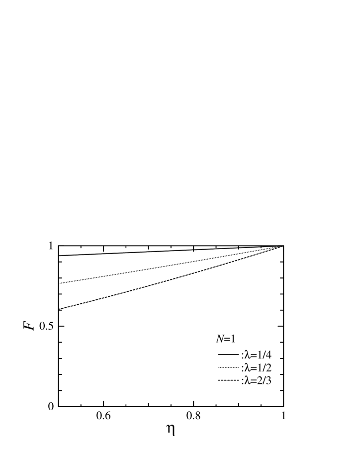
Figure 8: The fidelity $F_{\rm MSV}$ for the preparation of $N=1$ truncated maximally squeezed vacuum state $|\lambda=1,N=1\rangle$ is shown depending on $\eta$ with $\nu=0$. Some typical values are taken for the relevant squeezing parameter $\lambda$.

Figure 9: The fidelity $F_{\rm MSV}$ for the preparation of $N=2$ truncated maximally squeezed vacuum state $|\lambda=1,N=2\rangle$ is shown depending on $\eta$ with $\nu=0$. Some typical values are taken for the relevant squeezing parameter $\lambda$.

For generating the truncated maximally squeezed vacuum states,

$$|\lambda=1,N=1\rangle=(|0\rangle|0\rangle+|1\rangle|1\rangle)/{\sqrt{2}},$$

$$|\lambda=1,N=2\rangle=(|0\rangle|0\rangle+|1\rangle|1\rangle+|2\rangle|2\rangle)/{\sqrt{3}},$$

the generalized Bell state $|\phi_{-}(N,0,r=1/\lambda)\rangle$ and the squeezed vacuum state $|\lambda\rangle$ are taken as the input state and EPR resource, respectively. The matrix representing the input state is given by

$${\bf c}^{\rm in}={\bf E}[|\phi_{-}(N,0,r=1/\lambda)\rangle].$$

Then, the fidelity is calculated for example with $\lambda=1/4$ as

$$\Delta F_{\rm MSV}\equiv 1-F_{\rm MSV}[N=1;\lambda=1/4]:$$

$$\left[\begin{array}[]{ccc}a&f^{(a,0)}{\delta\eta}^{a}&f^{(a,1)}\nu{\delta\eta}^{a}\\ 0&-\!\!\!-\!\!\!-&0\\ 1&1/8&0\\ 2&-1/256&-1/8\\ 3&0&-7/64\\ 4&0&-225/2048\end{array}\right]\ ,$$ (195)

$$\Delta F_{\rm MSV}\equiv 1-F_{\rm MSV}[N=2;\lambda=1/4]:$$

$$\left[\begin{array}[]{ccc}a&f^{(a,0)}{\delta\eta}^{a}&f^{(a,1)}\nu{\delta\eta}^{a}\\ 0&-\!\!\!-\!\!\!-&0\\ 1&35/192&0\\ 2&-391/36864&-1351/4608\\ 3&-77/786432&-107425/442368\\ 4&8473/226492416&-4611707/18874368\end{array}\right]\ .$$ (202)

Numerical estimates are shown in Figs. 8 and 9 for $N=1$ and $N=2$, respectively, depending on $\eta$ with $\nu=0$ for simplicity, where some typical values are taken for the relevant squeezing parameter $\lambda$. The contributions of the dark count are actually negligible for $\nu\sim 10^{-4}$, since $f^{(0,1)}=f^{(1,1)}=0$ incidentally, as seen in the above lists. A fairly high fidelity $F_{\rm MSV}>0.94$ can really be achieved for $\eta\geq 0.7$ with small enough $\lambda\leq 1/4$. The input generalized Bell state $|\phi_{-}(N,0,r=1/\lambda)\rangle$ may be prepared from a pair of squeezed vacuum states $|\lambda^{\prime}\rangle$ and $|\lambda^{\prime\prime}\rangle$ with $r=\lambda^{\prime\prime}/\lambda^{\prime}=1/\lambda$. As seen so far, a high fidelity $F_{\rm GB}>0.95$ can be achieved for $\eta\geq 0.7$ with $\lambda^{\prime\prime}\leq 1/4$. Then, the actual net fidelity to prepare the truncated maximally squeezed vacuum state $|\lambda=1,N=1,2\rangle$ can be as high as 0.9, e.g., for $\eta=0.7$ with $\lambda=1/4$, $\lambda^{\prime}=(1/4)^{2}$ and $\lambda^{\prime\prime}=1/4$.

It should be remarked here that the input state and EPR state may be exchanged in the preparation of $|\lambda=1,N\rangle$. Then, the fidelity somewhat changes since the optical setup of Bell state detector is asymmetric under the exchange of the input modes 1 and 2, as explained before. In fact, we have $F_{\rm MSV}=1-f^{(0,1)}\nu+\ldots$ ($f^{(0,1)}\sim 10-50$) with $|\psi_{\rm in}^{(2)}\rangle=|\lambda\rangle$ and $|{\rm EPR}\rangle=|\phi_{-}(N,0,r=1/\lambda)\rangle$ for both the cases of $N=1,2$. It is really checked numerically that the corrections of the order of $\nu^{0}$ are zero up to ${\delta\eta}^{4}$ independent of $\lambda$. This case may be more favorable since the fidelity is rather insensitive to $\eta$. Furthermore, a somewhat large $\lambda$ may be taken to increase the success probability. The effect of the dark count is small enough for $\nu\sim 10^{-4}$ with $f^{(0,1)}\sim 50$. In any case, the fidelity for the preparation of $|\phi_{-}(N,0,r=1/\lambda)\rangle$ should be considered.

The net success probability to prepare $|\lambda=1,N\rangle$ from $|\phi_{-}(N,0,r=1/\lambda)\rangle$ and $|\lambda\rangle$ is estimated roughly KY-2003 as

$$P_{\rm MSV}(N)\sim\frac{p(N)^{2}}{(N+1)^{2}}\lambda^{\prime 2N},$$

where $\lambda^{\prime}=\lambda\lambda^{\prime\prime}$ with $\lambda^{2},\lambda^{\prime 2},\lambda^{\prime\prime 2}\ll 1$. Numerically, for example $P_{\rm MSV}(1)\sim 4\times 10^{-3}$ and $P_{\rm MSV}(2)\sim 7\times 10^{-6}$ with $\lambda=1/2$, $\lambda^{\prime}=1/8$ and $\lambda^{\prime\prime}=1/4$.

VI Summary

In summary, we have analyzed the linear optical realization of number-sum Bell measurement and number-state manipulation by taking into account the realistic experimental situation, specifically imperfectness of single-photon detector. The present scheme for number-state manipulation is based on the number-sum Bell measurement, which is implemented with linear optical elements, i.e., beam splitters, phase shifters and zero-one-photon detectors. Squeezed vacuum states and coherent states are used as optical sources, while single-photon sources may not be required. The linear optical Bell state detector has been formulated quantum theoretically with a probability operator measure. Then, the fidelity of manipulation and preparation of number-states, particularly for qubits and qutrits, has been evaluated in terms of the quantum efficiency $\eta$ and dark count $\nu$ of single-photon detector. It will be encouraging for future experimental attempts that a high fidelity is achievable for $\eta\gtrsim 0.7$ and $\nu\sim 10^{-4}$ with small enough squeezing parameters $\sim 0.1$ and coherent state amplitudes $\lesssim 1$.

References

• (1) C. H. Bennett, G. Brassard, C. Crepeau, R. Jozsa, A. Peres, and W. K. Wootters, Phys. Rev. Lett. 70, 1895 (1993).
• (2) S. L. Braunstein and H. J. Kimble, Phys. Rev. Lett. 80, 869 (1998); L. Vaidman, Phys. Rev. A 49, 1473 (1994).
• (3) G. J. Milburn and S. L. Braunstein, Phys. Rev. A 60, 937 (1999); P. T. Cochrane, G. J. Milburn, and W. J. Munro, Phys. Rev. A, 62, 062307 (2000); P. T. Cochrane and G. J. Milburn, Phys. Rev. A, 64, 062312 (2001).
• (4) D. T. Pegg, L. S. Phillips, and S. M. Barnett, Phys. Rev. Lett. 81, 1604 (1998); S. M. Barnett and D. T. Pegg, Phys. Rev. A 60, 4965 (1999).
• (5) M. Koniorczyk, Z. Kurucz, A. Gábris, and J. Janszky, Phys. Rev. A 62, 013802 (2000); C. J. Villas-Boas, Y. Guimarães, M. H. Y. Moussa, and B. Baseia, ibid. 63, 055801 (2001).
• (6) Ş. K. Özdemir, A. Miranowicz, M. Koashi, and N. Imoto, Phys. Rev. A 64, 063818 (2001); ibid. 66, 053809 (2002).
• (7) S. A. Babichev, J. Ries, and A. I. Lvovsky, Europhys. Lett. 64, 1 (2003).
• (8) E. Lombardi, F. Sciarrino, S. Popescu and F. De Martini, Phys. Rev. Lett. 88, 070402 (2002).
• (9) G. Björk and J. Söderholm, J. Opt. B: Quantum Semiclass. Opt. 1, 315 (1999).
• (10) A. Kitagawa and K. Yamamoto, Phys. Rev. A 66, 052312 (2002).
• (11) A. Kitagawa and K. Yamamoto, Phys. Rev. A 68, 042324 (2003).
• (12) X. B. Zou, K. Pahlke, and W. Mathis, Phys. Rev. A 68, 043819 (2003).
• (13) X. B. Zou, K. Pahlke, and W. Mathis, Phys. Lett. A 323, 329 (2004).
• (14) A. Trifonov, T. Tsegaye, G. Björk, J. Söderholm, E. Goober, M. Atatüre and A. V. Sergienko, J. Opt. B: Quantum Semiclass. Opt. 2, 105 (2000).
• (15) S. Takeuchi, J. Kim, Y, Yamamoto, and H. H. Hogue, Appl. Phys. Lett. 74, 1063 (1999); J. Kim, S. Takeuchi, Y. Yamamoto, and H. H. Hogue, ibid. 74, 902 (1999).
• (16) A. Imamoḡlu, Phys. Rev. Lett. 89, 163602 (2002); D. F. V. James and P. G. Kwiat, Phys. Rev. Lett. 89, 183601 (2002); M. Johnsson and M. Fleischhauer, Phys. Rev. A 67, 061802 (2003); K. Banaszek and I. A. Walmsley, Opt. Lett. 28, 52 (2003); D. Achilles, C. Silberhorn, C. Śliwa, K. Banaszek, and I. A. Walmsley, Opt. Lett. 28, 2387 (2003); O. Haderka, M. Hamar, and J. Peřina Jr., arXiv:quant-ph/0302154 (2003); J. Řeháček, Z. Hradil, O. Haderka, J. Peřina Jr., and M. Hamar, Phys. Rev. A 67, 061801 (2003); M. J. Fitch, B. C. Jacobs, T. B. Pittman, and J. D. Franson, Phys. Rev. A 68, 043814 (2003); A. M. Brańczyk, T. J. Osborne, A. Gilchrist, and T. C. Ralph, Phys. Rev. A 68, 043821 (2003).
• (17) A. Luis and L. L. Sánchez-Soto, Phys. Rev. A 48, 4702 (1993).
• (18) D. T. Pegg and S. M. Barnett, Phys. Rev. A 39, 1665 (1989); S. M. Barnett and D. T. Pegg, Phys. Rev. A 42, 6713 (1990).
• (19) H. Paul, P. Törmä, T. Kiss, and I. Jex, Phys. Rev. Lett. 76, 2464 (1996); P. Kok and S. L. Braunstein, Phys. Rev. A 63, 033812 (2001).
• (20) M. Reck, A. Zeilinger, H. J. Bernstein and P. Bertani, Phys. Rev. Lett. 73, 58 (1994).
• (21) S. M. Barnett, L. S. Phillips and D. T. Pegg, Opt. Comm. 158, 45 (1998) .