Quantum limited force measurement in a cavityless optomechanical system

Abstract

We study the possibility of revealing a weak coherent force by using a pendular mirror as a probe, and coupling this to a radiation field, which acts as the meter, in a cavityless configuration. We determine the sensitivity of such a scheme and show that the use of an entangled meter state greatly improves the ultimate detection limit. We also compare this scheme with that involving an optical cavity.

Optomechanical systems play a crucial role in a variety of precision measurement like gravitational wave detection GRAV and atomic force microscope AFM . They are based on the interaction between a movable mirror, a probe experiencing tiny forces, and a radiation field, a meter reading out the mirror’s position.

In these applications one needs very high resolution measurements and a good control of the various noise sources, because one has to detect the effect of very weak forces. In the simpler setup SETUP , optomechanical systems are usually intended as a Fabry-Perot cavity with a movable end mirror coupled to the external force and to the radiation probe. As shown by the pioneering work of Braginsky BRAG , even though all classical noise sources had been minimized, the detection of weak forces in such optomechanical systems would ultimately be determined by quantum fluctuations and the Heisenberg uncertainty principle. In particular, quantum noise has two fundamental sources, the photon shot noise of the laser beam, and the fluctuations of the mirror position due to radiation pressure. The two quantum noises determine the so-called standard quantum limit (SQL). It has been argued that the use of squeezed meter state allows to overcome the SQL CAV80 .

Here, differently from the standard optomechanical setup, SETUP , we do not consider an optical cavity but only a single mirror, illuminated by an intense and highly monochromatic optical beam. We shall derive the SQL for such a system and we shall show that it could be beaten by using entangled meters.

We consider a perfectly reflecting mirror and an intense quasi-monochromatic laser beam impinging on its surface (see Fig. 1). The laser beam is linearly polarized along the mirror surface and focused in such a way as to excite Gaussian acoustic modes of the mirror. These modes describe small elastic deformations of the mirror along the direction orthogonal to its surface and are characterized by a small waist, a large quality factor and a small effective mass PIN99 . It is possible to adopt a single vibrational mode description limiting the detection bandwidth to include a single mechanical resonance of frequency $\Omega$. In this description the incident laser beam, with frequency $\omega_{0}$, is reflected into an elastic carrier mode, with the same frequency $\omega_{0}$, and two additional weak anelastic sideband modes with frequencies $\omega_{0}\pm\Omega$ PRA1203 . The physical process is very similar to a stimulated Brillouin scattering, even though in this case the Stokes and anti-Stokes component are back-scattered by the acoustic wave at reflection, and the optomechanical coupling is provided by the radiation pressure. Treating classically the intense incident beam (and the carrier mode), the quantum system is composed of three interacting quantized bosonic modes, i.e. the vibrational mode and the two sideband modes. In our description, vibrational, Stokes and anti-Stokes modes are characterized by ladder operators $\hat{b}$, $\hat{a}_{1}$ and $\hat{a}_{2}$ respectively.

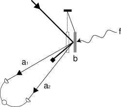
Figure 1: Schematic description of the studied system. A laser field at frequency $\omega_{0}$ impinges on the mirror vibrating at frequency $\Omega$. In the reflected field two sideband modes are excited at frequencies $\omega_{1}=\omega_{0}-\Omega$ and $\omega_{2}=\omega_{0}+\Omega$.

In PRA1203 an effective interaction Hamiltonian for that system has been derived as

$${\hat{H}}_{eff}=-i\hbar\chi\left({\hat{a}}_{1}{\hat{b}}-{\hat{a}}_{1}^{{\dagger}}{\hat{b}}^{{\dagger}}\right)-i\hbar\theta\left({\hat{a}}_{2}{\hat{b}}^{{\dagger}}-{\hat{a}}_{2}^{{\dagger}}{\hat{b}}\right)\,,$$ (1)

where $\chi$ and $\theta$ are couplings constants proportional to $\sqrt{\wp}$, with $\wp$ the incident laser power. Their ratio $\theta/\chi=\left[(\omega_{0}+\Omega)/(\omega_{0}-\Omega)\right]^{1/2}\geq 1$ only depends on the involved frequencies. The system dynamics is satisfactorily reproduced by the Hamiltonian of Eq. (1) as long as the dissipative coupling of the mirror vibrational mode with its environment is negligible. This happens if the interaction time is much smaller than the relaxation time of the vibrational mode and therefore it means having a high quality factor vibrational mode TIT99 .

We now consider the action of a classical coherent force on the probe and its readout through radiation fields. Since Eq.(1) is already written in a frame rotating at frequency $\Omega$ PRA1203 , if the force is constant, the total Hamiltonian would be

$$\hat{H}=\hat{H}_{eff}-\hbar\Omega f\left(\hat{b}e^{-i\Omega t}+\hat{b}^{\dagger}e^{i\Omega t}\right),$$ (2)

where $f$ denotes the dimensionless force strength. Eq.(2) leads to the following set of Heisenberg equations

$$\dot{\hat{a}}_{1} = \chi{\hat{b}}^{{\dagger}}\,,$$ (3a)

$$\dot{\hat{b}} = \chi{\hat{a}}_{1}^{{\dagger}}-\theta{\hat{a}}_{2}+i\Omega fe^{i\Omega t}\,,$$ (3b)

$$\dot{\hat{a}}_{2} = \theta{\hat{b}}\,,$$ (3c)

whose solutions read

$${\hat{a}}_{1}(t)=\frac{1}{\Theta^{2}}\left[\theta^{2}-\chi^{2}\cos\left(\Theta t\right)\right]{\hat{a}}_{1}(0)+\frac{\chi}{\Theta}\sin\left(\Theta t\right){\hat{b}}^{{\dagger}}(0)$$

$$-\frac{1}{\Theta^{2}}\left[\chi\theta-\chi\theta\cos\left(\Theta t\right)\right]{\hat{a}}_{2}^{{\dagger}}(0)$$

$$-\left[\Omega\sinh\left(\Theta t\right)-i\left(e^{-i\Omega t}-\cos\left(\Theta t\right)\right)\right]\frac{\Omega}{\Omega^{2}-\Theta^{2}}\chi f\,,$$ (4a)

$${\hat{b}}(t)=\frac{\chi}{\Theta}\sin\left(\Theta t\right){\hat{a}}_{1}^{{\dagger}}(0)+\cos\left(\Theta t\right){\hat{b}}(0)$$

$$-\frac{\theta}{\Theta}\sin\left(\Theta t\right){\hat{a}}_{2}(0)$$

$$-\left[\Omega\cos\left(\Theta t\right)+i\Theta\sin\left(\Theta t\right)+\Omega e^{i\Omega t}\right]\frac{\Omega}{\Omega^{2}-\Theta^{2}}f\,,$$ (4b)

$${\hat{a}}_{2}(t)=\frac{1}{\Theta^{2}}\left[\chi\theta-\chi\theta\cos\left(\Theta t\right)\right]{\hat{a}}_{1}^{{\dagger}}(0)+\frac{\theta}{\Theta}\sin\left(\Theta t\right){\hat{b}}(0)$$

$$-\frac{1}{\Theta^{2}}\left[\chi^{2}-\theta^{2}\cos\left(\Theta t\right)\right]{\hat{a}}_{2}(0)$$

$$-\left[\Omega\sin\left(\Theta t\right)+i\left(e^{i\Omega t}-\cos\left(\Theta t\right)\right)\right]\frac{\Omega}{\Omega^{2}-\Theta^{2}}\theta f\,,$$ (4c)

with $\Theta=\sqrt{\theta^{2}-\chi^{2}}$.

We consider the mirror initially in a thermal state QOPT

$$\hat{\rho}_{b}=\frac{1}{1+{\cal N}_{th}}\sum_{n}\left(\frac{{\cal N}_{th}}{1+{\cal N}_{th}}\right)^{n}|n\rangle\langle n|\,,$$ (5)

where the mean number of thermal excitations is given by

$${\cal N}_{th}=\frac{1}{e^{\hbar\Omega/k_{B}T}-1}\,.$$ (6)

with $k_{B}$ the Boltzmann constant and $T$ the equilibrium temperature. Furthermore, quite generally, we assume the meter modes initially in a pure state of the form

$$|\Psi\rangle_{12}=\sqrt{1-\tanh^{2}s}\sum_{n=0}^{\infty}\left(\tanh s\right)^{n}|n\rangle_{1}\,|n\rangle_{2}\,,$$ (7)

with the parameter $s\in{\bf R}$. This state for $s=0$ gives the tensor product of vacuum state for the two sideband modes, instead, if $s\neq 0$ it represents a two mode squeezed state QOPT , which shows entanglement. In that case the two meter modes ${\hat{a}}_{1}$ and ${\hat{a}}_{2}$ are not initially empty, thus, they could in turn excite their own sideband modes with coupling costants say $\chi_{1,2}$ and $\theta_{1,2}$. The latter are proportional to the corresponding powers $\wp_{1,2}$ of the modes ${\hat{a}}_{1}$, ${\hat{a}}_{2}$ determined by $\sinh^{2}s$ QOPT . We assume that $\wp\gg\wp_{1,2}$, hence $\chi,\,\theta\gg\chi_{1,2},\,\theta_{1,2}$, so that in Eq.(1) we neglected terms related to $\chi_{1,2}$ and $\theta_{1,2}$. However, to not neglect the force term in Eq.(2), we also require the condition $\Omega f\gg\chi_{1,2},\,\theta_{1,2}$ to be satisfied.

Let us now consider the heterodyne detection YS on the reflected sideband modes ${\hat{a}}_{1}$, ${\hat{a}}_{2}$. That is, we consider the possibility to simultaneously measure the real and the imaginary part of the operator

$$\hat{Z}_{\varphi}=\hat{a}_{1}e^{i\varphi}-\hat{a}_{2}^{\dagger}e^{-i\varphi}\,,$$ (8)

where $\varphi$ is a phase that can be experimentally adjusted. We now introduce the amplitude and phase quadratures for the two optical modes as $\hat{X}_{j}=(\hat{a}_{j}+\hat{a}_{j}^{{\dagger}})/{2}$, $\hat{Y}_{j}=-i(\hat{a}_{j}-\hat{a}_{j}^{{\dagger}})/{2}$, $j=1,2$, with commutation relation $[\hat{X}_{j},\hat{Y}_{k}]=\delta_{jk}/2$. Then, it is well known QOPT that the state (7) with $s\neq 0$ allows reduced variances for $\hat{X}_{1}-\hat{X}_{2}$ and $\hat{Y}_{1}+\hat{Y}_{2}$ with respect to the case of $s=0$. This could be fruitfully exploited to reduce the noise on the readout. Inspired by this fact we choose $\varphi=\pi$ in Eq.(8) and obtain

$$\hat{Z}_{\pi}=-\left(\hat{X}_{1}-\hat{X}_{2}\right)-{i}\left(\hat{Y}_{1}+\hat{Y}_{2}\right)\,.$$ (9)

More specifically, we shall consider only the imaginary part of $\hat{Z}_{\pi}$, which, by virtue of Eqs.(9) and (4), results

$$\hat{Z}_{I}(t)=\frac{\left(\theta-\chi\right)}{\Theta^{2}}\left[\theta+\chi\cos\left(\Theta t\right)\right]\hat{Y}_{1}(0)$$

$$+\frac{\left(\theta-\chi\right)}{\Theta^{2}}\left[\chi+\theta\cos\left(\Theta t\right)\right]\hat{Y}_{2}(0)$$

$$+\frac{\left(\theta-\chi\right)}{\Theta}\sin\left(\Theta t\right)\left[\frac{\hat{b}(0)-\hat{b}^{{\dagger}}(0)}{2i}\right]$$

$$+\left(\theta-\chi\right)\left[\cos\left(\Theta t\right)-\cos\left(\Omega t\right)\right]\frac{\Omega}{\Omega^{2}-\Theta^{2}}f\,.$$ (10)

Then, the signal, using Eqs.(5) and (7), will be

$$\langle Z_{I}\rangle\equiv{\cal S}f=\left(\theta-\chi\right)\left[\cos\left(\Theta t\right)-\cos\left(\Omega t\right)\right]\frac{\Omega}{\Omega^{2}-\Theta^{2}}f\,,$$ (11)

while the noise

$$\langle Z_{I}^{2}\rangle-\langle Z_{I}\rangle^{2}\equiv{\cal N}$$

$$=\frac{-1}{4\Theta^{4}}\bigg{[}2\theta\chi\left(\theta^{2}+\chi^{2}\right)\left(1-\cos\left(\Theta t\right)\right)^{2}+8\theta^{2}\chi^{2}\cos\left(\Theta t\right)$$

$$-\left(\theta^{2}+\chi^{2}\right)^{2}\left(1+\cos^{2}\left(\Theta t\right)\right)\bigg{]}\left(1+2\sinh^{2}(s)\right)$$

$$-\,\frac{1}{2\Theta^{4}}\bigg{[}-\left(\theta^{2}+\chi^{2}\right)^{2}\cos\left(\Theta t\right)+2\theta^{2}\chi^{2}\left(1+\cos^{2}\left(\Theta t\right)\right)$$

$$-\theta\chi\left(\theta^{2}+\chi^{2}\right)\left(1-\cos\left(\Theta t\right)\right)^{2}\bigg{]}\left(\sinh(2s)\right)$$

$$+\frac{\left(\theta-\chi\right)^{2}}{4\Theta^{2}}\sin^{2}\left(\Theta t\right)\left(1+2{\cal N}_{th}\right).$$ (12)

The relevant quantity determining the sensitivity of the system is the signal to noise ratio (SNR)

$${\cal R}=\frac{|{\cal S}|}{\sqrt{{\cal N}}}f\,,$$ (13)

which must be $\geq 1$ to reveal the force. Hence, the condition ${\cal R}=1$ gives the minimum detectable force, i.e.

$$f_{min}=\frac{\sqrt{{\cal N}}}{|{\cal S}|}\,.$$ (14)

We can see that the thermal noise increases the values assumed by $f_{min}$ for all times, but for $\Theta t=\pi$ it gives no contribution. At that time we have

$$f_{min}(\Theta t=\pi)=\frac{\Omega^{2}-\Theta^{2}}{\theta+\chi}\frac{e^{-s}}{\sqrt{2}\Omega\left(1-\cos\left(\pi\Omega/\Theta\right)\right)}\,,$$ (15)

which shows the possibility to improve the sensitivity by using entanglement (provided $\Omega/(2\Theta)$ not integer).

Now, we compare our model with that involving a single mode optical cavity. We consider an intense laser beam (of power $\wp$) exciting a single cavity mode and realizing, in the semiclassical approximation the effective Hamiltonian EPL03

$$\hat{H}_{eff}=-\hbar\Delta\hat{a}^{{\dagger}}\hat{a}+\hbar\Omega\hat{b}^{{\dagger}}\hat{b}+\hbar g\left(\alpha^{*}\hat{a}+\alpha\hat{a}^{{\dagger}}\right)\left(\hat{b}+\hat{b}^{{\dagger}}\right)\,,$$ (16)

where $\alpha\propto\sqrt{\wp}$ denotes the classical cavity field amplitude, $\Delta$ the cavity detuning, $g$ the optomechanical coupling, and $\hat{a}$ the radiation field quantum fluctuations. The meaning of the other symbols is the same as in the main text. By adding the driving $-\hbar\Omega f\left(\hat{b}+\hat{b}^{{\dagger}}\right)$ to Eq.(16), we are led to the following Heisenberg equations

$$\dot{\hat{a}} = i\Delta\hat{a}-ig\alpha\left(b+b^{{\dagger}}\right)\,,$$ (17a)

$$\dot{\hat{b}} = -i\Omega\hat{b}-ig\left(\alpha^{*}\hat{a}+\alpha\hat{a}^{{\dagger}}\right)+i\Omega f\,,$$ (17b)

Choosing $\Delta=0$, $\alpha\in{\bf R}$, and introducing the field quadratures ${\hat{X}}=(\hat{a}+\hat{a}^{{\dagger}})/{2}$, ${\hat{Y}}=-i(\hat{a}-\hat{a}^{{\dagger}})/{2}$, we immediately see that only the phase quadrature $\hat{Y}$ carries out information about the force. As a matter of fact, from Eqs.(17), we obtain

$$\hat{Y}(t)=-\frac{g\alpha}{\Omega}\sin\left(\Omega t\right)\left(\hat{b}(0)+\hat{b}^{{\dagger}}(0)\right)$$

$$+i\frac{g\alpha}{\Omega}\left[1-\cos\left(\Omega t\right)\right]\left(\hat{b}(0)-\hat{b}^{{\dagger}}(0)\right)$$

$$+\left(\frac{2g\alpha}{\Omega}\right)^{2}\left[\Omega t-\sin\left(\Omega t\right)\right]\hat{X}(0)$$

$$+\frac{2g\alpha}{\Omega}\left[\Omega t-\sin\left(\Omega t\right)\right]f+\hat{Y}(0)\,.$$ (18)

As the initial state we consider the thermal state (5) for the probe and a squeezed state for the meter, i.e. $\exp[\zeta^{*}(\hat{a})^{2}-\zeta({\hat{a}}^{{\dagger}})^{2}]|0\rangle$ with $\zeta=(s/2)\exp(2i\phi)$ the squeezing parameter QOPT .

Since we are considering the good cavity limit Note , we restrict our analysis to only the cavity mode and suppose to be able to perform its homodyne detection HOM . One then gets the following signal

$$\langle\hat{Y}(t)\rangle\equiv{\cal S}(t)\,f=\frac{2g\alpha}{\Omega}\left[\Omega t-\sin\left(\Omega t\right)\right]\,f\,.$$ (19)

The corresponding noise can be calculated by means of the initial thermal state of the probe, and the squeezed state for the meter. Thus, we get

$$\left\langle\hat{Y}^{2}(t)\right\rangle-\langle\hat{Y}(t)\rangle^{2}\equiv{\cal N}(t)$$ (20)

$$=\left(\frac{g\alpha}{\Omega}\right)^{2}\sin^{2}\left(\Omega t\right)\left({1}+2{\cal N}_{th}\right)$$

$$+\left(\frac{g\alpha}{\Omega}\right)^{2}\left[1-\cos\left(\Omega t\right)\right]^{2}\left({1}+2{\cal N}_{th}\right)$$

$$+\left(2\frac{g\alpha}{\Omega}\right)^{4}\left[\Omega t-\sin\left(\Omega t\right)\right]^{2}\left[e^{-2s}\cos^{2}\phi+e^{2s}\sin^{2}\phi\right]$$

$$+\left[e^{-2s}\sin^{2}\phi+e^{2s}\cos^{2}\phi\right]$$

$$+2\left(\frac{2g\alpha}{\Omega}\right)^{2}\left[\Omega t-\sin\left(\Omega t\right)\right]\left[e^{2s}-e^{-2s}\right]\sin\phi\cos\phi\,.$$

It is easy to see that at times such that $\Omega t=2\pi$ the thermal noise does not contribute. Then, minimizing over $\phi$ we get for such times

$${\cal N}_{min}(\Omega t=2\pi)=\left[1+4\pi^{2}\left(\frac{2g\alpha}{\Omega}\right)^{4}\right]e^{-2s}\,,$$ (21)

that is

$$f_{min}(\Omega t=2\pi)=\frac{\left[1+4\pi^{2}\left(2g\alpha/\Omega\right)^{4}\right]^{1/2}}{4\pi\left(g\alpha/\Omega\right)}e^{-s}\,.$$ (22)

The minimum detectable force, for each of the models, is shown in Fig.2 as a function of time for different values of $s$ and ${\cal N}_{th}$. In both cases $f_{min}$ for ${\cal N}_{th}=s=0$ represents the SQL. For the cavityless model (top plot), we notice oscillations due to the presence of two different frequencies $\Theta$, $\Omega$ in Eq.(11), while for the cavity model (bottom plot) the oscillations only depend on the mirror frequency $\Omega$. We can see that for all times in which the mirror is disentangled from the radiation, Eq. (15) and Eq.(22) show the possibility to go beyond the SQL. Note that Fig. 2 represents only a “qualitative” comparison between the two models.

Looking at the scaling in terms of the laser power, in both Eqs. (15) and (22) we recognize the same contributions: $\frac{1}{\sqrt{\wp}}$ due to the shot noise (prevealing at small laser power), and $\sqrt{\wp}$ due to the radiation pressure noise (prevealing at large laser power). Anyway the two contributions are combined in a different manner; for the optical cavity model we have $f_{min}\propto\sqrt{\frac{1}{\wp}+\wp}$, while in the cavityless optomechanical model we have $f_{min}\propto\frac{1}{\sqrt{\wp}}-\sqrt{\wp}$. In the latter case, it seems that $f_{min}$ could be reduced to $0$ by simply choosing a proper value of $\wp$. This could happen for $\Omega^{2}-\Theta^{2}=0$, which however invalidates our model, since the Hamiltonian (1) has been derived in the limit $\Omega^{2}\gg\Theta^{2}$ PRA1203 . Moreover $f_{min}$ cannot go to $0$, because of the condition $\Omega f\gg\chi_{1,2},\,\theta_{1,2}$ which requires a large enough frequency $\Omega$ in order to beat the SQL (this condition holds e.g. for the parameters values of Fig.2).

It should be noted that in the cavityless model the time is essentially set by the incident optical pulse length. Therefore, it is particularly suited to perform pulsed measurement on the probe, while the cavity model presupposes a stationary condition between meter and probe, hence measurement on a long time scale. In both cases the use of a nonclassical meter state allows improvement of the performances only for particular interaction times, while the use of a nonclassical probe state would allow such improvement for almost all times HOL79 ; EPL03 .

In conclusion, we have presented a cavityless optomechanical model to reveal weak coherent forces and we have compared it with a cavity one. In particular, we have shown that nonclassical meter states allow one to beat the SQL greatly improving the sensitivity. Thus, we have shown that entanglement in a cavityless optomechanical scheme plays almost the same role as does squeezing in one which use a cavity. Finally, the cavityless optomechanical model could be useful in a number of applications, especially those involving micro-opto-mechanical-sensors MOMS .

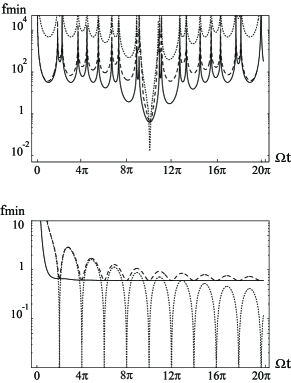
Figure 2: Log plot of the minimum detectable force versus scaled time $\Omega t$, for the cavityless model (top plot), and for the cavity model (bottom plot). In each plot the continous line represents the SQL; the dashed line refers to ${\cal N}_{th}=300$ and $s=0$; the dotted line refers to ${\cal N}_{th}=300$ and $s=5$. The values of other parameters are: $\theta/\chi=1.025$, $\Omega/\Theta\simeq 10$, $g\alpha/\Omega=0.2$.

References

• (1) A. Abramovici, et al., Science 256, 325 (1992); R. Loudon, Phys. Rev. Lett. 47, 815 (1981).
• (2) J. Mertz, et al., Appl. Phys. Lett. 62, 2344 (1993); T. D. Stowe, et al., Appl. Phys. Lett. 71, 288 (1997).
• (3) S. Mancini and P. Tombesi, Phys. Rev. A 49, 4055 (1994); C. Fabre, et al., Phys. Rev. A 49, 1337 (1994); G.J. Milburn, K. Jacobs, D. F. Walls Phys. Rev. A 50, 5256 (1994); C. K. Law, Phys. Rev. A 51, 1537 (1995); S. P. Vyatchanin and A. B. Matsko, J. Exp. Theor. Phys. 82, 1007 (1996); 83, 690 (1996); S. Mancini, V. I. Man’ko and P. Tombesi, Phys. Rev. A 55, 3042 (1997); S. Bose, K. Jacobs and P. L. Knight, Phys. Rev. A 56, 4175 (1997); K. Jacobs, et al., Phys. Rev. A 60, 538 (1999); V. Giovannetti and D. Vitali, Phys. Rev. A 63, 023812 (2001). D. Vitali, et al., Phys. Rev. A 65, 063803 (2002).
• (4) V. B. Braginsky and F. Ya Khalili, Quantum Measurements, (Cambridge University Press, Cambridge, 1992).
• (5) C. M. Caves, Phys. Rev. Lett. 45, 75 (1980); R. S. Bondurant and J. H. Shapiro, Phys. Rev. D 30, 2548 (1984); A. F. Pace, M. J. Collett and D. F. Walls, Phys. Rev. A 47, 3173 (1993).
• (6) M. Pinard, et al., Eur. Phys. J. D 7, 107 (1999).
• (7) S. Pirandola, S. Mancini, D. Vitali, P. Tombesi, Phis. Rev. A 68, 062317 (2003).
• (8) I. Tittonen, et al., Phys. Rev. A 59, 1038 (1999).
• (9) D. F. Walls and G. J. Milburn, Quantum Optics, (Springer, Berlin, 1994).
• (10) H. P. Yuen and J. H. Shapiro, IEEE Trans. Info. Theory IT-26, 78 (1980).
• (11) A. N. Cleland and M. L. Roukes, Nature(London) 392, 168 (1998); H. J. Mamin and D. Rugar, Appl. Phys. Lett. 79, 3358 (2001).
• (12) J. N. Hollenhorst, Phys. Rev. D 19, 1669 (1979).
• (13) S. Mancini and P. Tombesi, Europhys. Lett. 61, 8 (2003).
• (14) Notice that the model of Eq.(1) cannot be trivially obtained as the bad cavity limit of Eq.(16), because the two Hamiltonians have been derived under different assumptions, see e.g. Refs. SETUP ; PRA1203 .
• (15) H. M. Wiseman and G. J. Milburn, Phys. Rev. A 47, 642 (1993).