Causality, Entanglement, and Quantum Evolution Beyond Cauchy Horizons

Abstract

We consider a bipartite entangled system half of which falls through the event horizon of an evaporating black hole, while the other half remains coherently accessible to experiments in the exterior region. Beyond complete evaporation, the evolution of the quantum state past the Cauchy horizon cannot remain unitary, raising the questions: How can this evolution be described as a quantum map, and how is causality preserved? The answers are subtle, and are linked in unexpected ways to the fundamental laws of quantum mechanics. We show that terrestrial experiments can be designed to constrain exactly how these laws might be altered by evaporation.

Standard proofs that non-local Bell correlations bellcorr between parts of an entangled system cannot be used to acausally signal (transfer information) rely on quantum evolution being everywhere unitary. However, as Hawking hawkingnonunit first pointed out when he gave examples of non-unitary but causal maps for evaporating black holes, unitarity, a sufficient but not a necessary condition for causality, may break down in the late stages of black-hole evaporation. In this letter we ask: When entangled systems partly cross the event horizons of evaporating black holes (or Cauchy horizons of other, more general naked singularities) and partly remain coherently accessible to experiments outside, what constraints on their non-unitary, and possibly nonlinear quantum evolution would ensure causality? and: Can signaling (acausal) evolution be detected at large distances if it indeed does take place under the extreme conditions near naked singularities and evaporating black-hole interiors?

Why expect the experimentally well-established law of unitary evolution to break down during black-hole evaporation? Consider, for definiteness, a pure quantum-field state which gravitationally collapses to form an evaporating Schwarzschild black hole (Fig. 1).

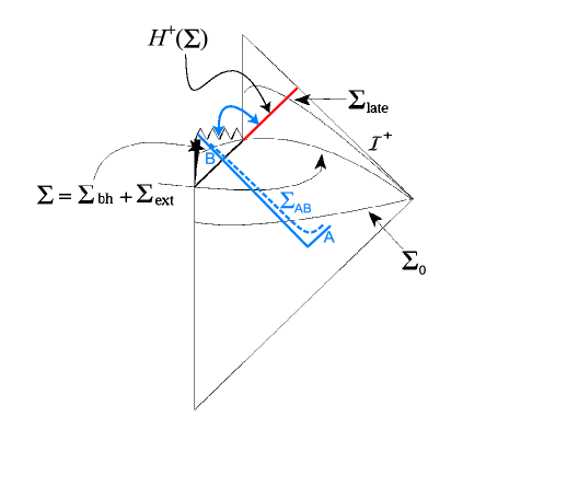
Figure 1: Conformal diagram illustrating the causal structure of a spacetime with an evaporating black hole (vertical lines on the left depict the axes of rotational symmetry). [The causal geometry illustrated by the superimposed blue drawing refers to the second paragraph following Eq. (15) below.] The spacelike hypersurface $\Sigma_{0}$ passes through the collapsing star before the black hole has formed, $\Sigma$ is a surface through the black hole just before it evaporates, and $\Sigma_{\rm late}$ is a surface at late times, after complete evaporation. The red line illustrates the Cauchy horizon $H^{+}(\Sigma)$ for $\Sigma$ or $\Sigma_{0}$; it is the future null cone of the “point” (really a singularity) of complete evaporation. Because evaporation is largely thermal, quantum evolution through $H^{+}(\Sigma)$ from the time slice $\Sigma_{0}$ to the slice $\Sigma_{\rm late}$ cannot be described as a unitary map.

Initially given by $|\Psi_{0}\rangle$ on the (partial) Cauchy surface $\Sigma_{0}$ in Fig. 1, the state evolves unitarily (at least in semiclassical gravity) during and after gravitational collapse: at any intermediate time slice $\Sigma$, it can be written as $|\Psi_{\Sigma}\rangle=U_{\Sigma\,\Sigma_{0}}|\Psi_{0}\rangle$, where $U_{\Sigma\,\Sigma_{0}}$ is the unitary time evolution operator acting on the Fock space of field states. An external observer in the asymptotically flat region outside the event horizon has no causal communication with the interior $\Sigma_{\rm bh}$; she would describe the state of the quantum field by the reduced density matrix

$$\rho_{\rm ext}={\rm Tr}_{\Sigma_{\rm bh}}\,|\Psi_{\Sigma}\rangle\,\langle\Psi_{\Sigma}|\;$$ (1)

obtained by tracing over the interior field degrees of freedom inside the horizon. As the black hole settles down to a stationary state on the time slice $\Sigma$, the mixed state $\rho_{\rm ext}$ can be shown (via non-trivial calculation bhentropy ) to approach precisely a thermal state $\rho_{H}$ at the Hawking temperature $T_{H}=\mathchar 1406\relax c^{3}/(8\pi k_{B}GM)$, where $M$ is the hole’s mass. As long as the back action of the Hawking radiation on spacetime is negligible (an eternal black hole), matter remains in the pure state $|\Psi_{\Sigma}\rangle$, which unitarily evolves to become entangled with its collapsed half inside the emerging event horizon. But what happens at late times, after this back action eventually destroys the black hole completely? In semiclassical gravity, it is impossible to escape the conclusion that the state $\rho_{\rm late}$ of the field on the late time slice $\Sigma_{\rm late}$ (Fig. 1) is mixed: $\rho_{\rm late}\approx\rho_{H}$. The resulting evolution $|\Psi_{0}\rangle\longmapsto\rho_{\rm late}$ cannot be unitary, as it maps pure states into mixed states. This inevitable breakdown of unitarity can only be avoided by postulating a remnant that persists at late times, continuing to carry the correlations “lost” in the state $\rho_{\rm late}$ by remaining entangled with the outgoing Hawking radiation.

The lesson we draw is: compared to the conditions encountered in local laboratory physics, conditions in the interiors of evaporating black holes are so extreme that the ordinary laws of quantum evolution may be profoundly altered ftnote1 . What kinds of non-unitary quantum dynamics might govern entangled multi-partite systems as their subsystems cross the Cauchy horizons of evaporating black holes? We argue that this dynamics must be probability-preserving, it can be (generally) nonlinear, and it must be local. The class of non-unitary maps (“superscattering operators”) discussed by Hawking hawkingnonunit is obtained via the additional constraint of linearity. We will show that linearity (along with probability conservation and locality) is sufficient to preserve causality ftnote2 ; acausal signaling is possible only with nonlinear maps. Nonlinear generalizations of quantum mechanics and their implications for measurement theory and causality have been discussed by many authors nlrefs ; it is not our goal in this letter to contribute to these developments. We adopt the conservative position that at most a minimal generalization of quantum theory—namely one that allows for the possibility of nonlinear quantum maps while keeping the rest of the formalism intact—is necessary to understand the non-standard quantum dynamics of black-hole evaporation. There is, of course, no experimental evidence for quantum nonlinearity under local laboratory conditions weinberg ; however, whether linearity continues to hold under the extreme conditions of evaporating black-hole interiors is a question yet to be decided by experiment. Remarkably, a simple terrestrial experiment can be designed to probe this question as we now discuss.

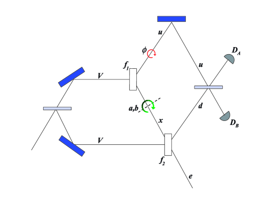
Figure 2: The Zou-Wang-Mandel interferometer mandeletal for the trans-horizon Bell-correlation experiment. Gray rectangles are 50:50 beam splitters, white rectangles are the two nonlinear parametric down-converting crystals with efficiencies $f_{1}$, $f_{2}$; blue rectangles are mirrors. A phase delay is placed on the idler beam labeled $u$, and an adjustable-angle polarization rotator is placed on the signal beam $x$ which is aligned with the second signal beam labeled $e$. Since both pump beams are blocked past the nonlinear crystals, the output state lies in the Hilbert space ${\cal H}_{u}\otimes{\cal H}_{d}\otimes{\cal H}_{e}$ of the signal and idler beams; it is monitored by the single-photon detectors $D_{A}$ and $D_{B}$.

Consider the optical setup schematically illustrated in Fig. 2, a straightforward modification of a well-known Bell-correlation experiment by Mandel et. al. mandeletal The pump beam (typically from the output of a uv-argon laser) is split into two beams which interact with two separate nonlinear crystals to produce correlated photons in two pairs of idler and signal beams, labeled $u$, $x$, and $d$, $e$, respectively. The key feature in the design of the experiment is the alignment of the first signal beam $x$ with the second signal beam $e$, which makes photon number-states in the beams (modes) $x$ and $e$ indistinguishable (in practice, the alignment needs to be accurate only to within the transverse laser coherence length). In the actual experiment the first signal beam $x$ may pass through the second nonlinear crystal as a consequence of its alignment with $e$, but its probability of further down-conversion, proportional to $|Vf_{1}f_{2}|^{2}$, is negligible since $|f_{i}|\ll 1$ and $|Vf_{i}|\ll 1$, $i=1,\;2$, where $V$ is the dimensionless amplitude of each of the two pump-beam pulses (photon number $\propto|V|^{2}$). We shall assume that both nonlinear crystals produce down-converted photons in a fixed (linear) polarization state. The quantum state output by this configuration belongs to the Hilbert space ${\cal H}\equiv{\cal H}_{u}\otimes{\cal H}_{d}\otimes{\cal H}_{e}$, where the “up” and “down” idler-beam Hilbert spaces are generated by the orthonormal basis states

$${\cal H}_{u}\equiv<\{|0\rangle_{u},\;|1\rangle_{u}\}>\;,\;\;\;\;{\cal H}_{d}\equiv<\{|0\rangle_{d},\;|1\rangle_{d}\}>\;,$$ (2)

and the “escaping” signal-beam Hilbert space is generated by the basis states

$${\cal H}_{e}\equiv<\{|0\rangle_{e},\;|1\rangle_{e},\;|-1\rangle_{e}\}>\;,$$ (3)

where $|0\rangle$ denotes the vacuum, $|1\rangle$ denotes the single-photon state in the original (linear) polarization mode produced by the down-conversion, and $|-1\rangle$ denotes the single-photon state in the orthogonal polarization mode, which is mixed into ${\cal H}_{e}$ by the polarization rotator (with complex coefficients $a$, $b$) placed along the signal beam $x$ (Fig. 2). The output state can be written as

$$|\psi\rangle = [\;|0\rangle_{u}|0\rangle_{d}|0\rangle_{e}$$ (4)

$$+ Vf_{1}e^{i\phi}\,|1\rangle_{u}|0\rangle_{d}\,(\;a\,|1\rangle_{e}\,+\,b\,|-1\rangle_{e}\;)$$

$$+ Vf_{2}\,|0\rangle_{u}|1\rangle_{d}|1\rangle_{e}\;]\,/\,N\;\;,$$

where $|a|^{2}+|b|^{2}=1$, and $N$ is the normalization factor

$$N\equiv\sqrt{1+|V|^{2}(|f_{1}|^{2}+|f_{2}|^{2})}\;.$$ (5)

Notice that the contributions from the signal beam $x$ and from the signal beam $e$ are coherently superposed in the output state $|\psi\rangle$ along the ${\cal H}_{e}$-direction in ${\cal H}$; this is the key consequence of aligning the two signal beams.

The experiment consists of monitoring the entangled output $|\psi\rangle$ at the two single-photon detectors $D_{A}$ and $D_{B}$. For the purposes of our essentially conceptual discussion in this letter, experimental inaccuracies and noise (detector inefficiencies, dark-count rates, $\ldots$) are not relevant, and we will defer their discussion to a forthcoming paper moretocome . Thus, measurement by the perfect detector $D_{A}$ is equivalent to the projection $P_{A}=P_{\alpha}\otimes\mathbb{I}_{e}$, where $\alpha\in{\cal H}_{u}\otimes{\cal H}_{d}$ is the vector $\alpha=(|0\rangle_{u}|1\rangle_{d}+i|1\rangle_{u}|0\rangle_{d})/{\sqrt{2}}$, and a measurement (click) at $D_{B}$ is equivalent to the projection $P_{B}=P_{\beta}\otimes\mathbb{I}_{e}$, where $\beta=(|1\rangle_{u}|0\rangle_{d}+i|0\rangle_{u}|1\rangle_{d})/{\sqrt{2}}$. Calculation [using $p_{A,\;B}={\rm Tr}(P_{A,\;B}|\psi\rangle\langle\psi|)=\|P_{A,\;B}|\psi\rangle\|^{2}$] shows that the probabilities $p_{A}$ and $p_{B}$ of clicks at detectors $D_{A}$ and $D_{B}$, respectively, are given by

$$p_{A} = \frac{|V|^{2}}{2\,N^{2}}\left[\,|f_{1}|^{2}+|f_{2}|^{2}\,+\,2\,\Re\,(\,i\overline{f_{1}}f_{2}\bar{a}e^{-i\phi}\,)\,\right]\;,$$

$$p_{B} = \frac{|V|^{2}}{2\,N^{2}}\left[\,|f_{1}|^{2}+|f_{2}|^{2}\,-\,2\,\Re\,(\,i\overline{f_{1}}f_{2}\bar{a}e^{-i\phi}\,)\,\right]\;.$$ (6)

The important feature in Eqs. (6) is the interference term in brackets following the real-part sign $\Re$. Notice that the interference is oscillatory in the controlled phase delay $\phi$ and depends sensitively on the polarization angles $(a,b)$.

But how does the interference depend on the evolution of the probe beam $e$ which escapes to infinity? Let $\rho_{ud}\equiv{\rm Tr}_{e}|\psi\rangle\langle\psi|$ be the output state projected on the “laboratory” Hilbert space ${\cal H}_{u}\otimes{\cal H}_{d}$. It is straightforward to show that the detection probabilities $p_{A,\;B}$ can be alternatively computed via the expressions $p_{A,\;B}={\rm Tr}_{ud}(P_{\alpha,\;\beta}\,\rho_{ud})$. This result is, of course, valid much more generally: the expectation value of any observable $O=O_{ud}\otimes\mathbb{I}_{e}$ (i.e. one local to the Hilbert space ${\cal H}_{u}\otimes{\cal H}_{d}$) depends only on the reduced state projected on ${\cal H}_{u}\otimes{\cal H}_{d}\;$:

$${\rm Tr}\,[\,(O_{ud}\otimes\mathbb{I}_{e})\,|\psi\rangle\langle\psi|\,]={\rm Tr}_{ud}\,[\,O_{ud}\,{\rm Tr}_{e}|\psi\rangle\langle\psi|\,]\;.$$ (7)

Now suppose that the output state $|\psi\rangle$ undergoes a local quantum evolution (local in the sense that ${\cal E}={\cal E}_{ud}\otimes{\cal E}_{e}$)

$${\cal E}={\cal E}_{ud}\otimes{\cal E}_{e}\;:\;|\psi\rangle\langle\psi|\mapsto({\boldsymbol{1}}_{ud}\otimes{\cal E}_{e})(|\psi\rangle\langle\psi|)\;,$$ (8)

where ${\cal E}_{e}$ is an arbitrary, completely-positive, linear quantum map on ${\cal H}_{e}$-states which is probability preserving, with Kraus representation:

$${\cal E}_{e}:\rho\mapsto\sum_{j}E_{j}\rho{E_{j}}^{\dagger}\;,\;\;\;\;\;\sum_{j}{E_{j}}^{\dagger}E_{j}=\mathbb{I}_{e}\;,$$ (9)

where $E_{j}$ are otherwise arbitrary linear operators on ${\cal H}_{e}$. For any state $\rho$ on ${\cal H}$ [including the output state $\rho=|\psi\rangle\langle\psi|$ of Eq. (4)], by expanding $\rho$ in the form $\rho=\sum_{\mu}c_{\mu}\,{\rho_{ud}}^{(\mu)}\otimes{\sigma_{e}}^{(\mu)}$, $c_{\mu}\in\mathbb{R}$, it is straightforward to prove the identity

$${\rm Tr}_{e}\,[\,({\boldsymbol{1}}_{ud}\otimes{\cal E}_{e})\rho\,]={\rm Tr}_{e}\rho$$ (10)

for any linear map ${\cal E}_{e}$ of the form Eq. (9). In view of Eq. (7), Eq. (10) is the expression of causality (no-signaling; compare Eq. (15) below): As long as the evolution of the probe beam $e$ remains linear and probability-conserving, the interference pattern of the laboratory beams does not depend on what happens to $e$. The detection probabilities $p_{A}$ and $p_{B}$ are given by Eqs. (6) whether $e$ evolves unitarily, is absorbed in a beam block, or otherwise gets entangled with the rest of the universe.

By contrast, suppose that the beam $e$ undergoes a nonlinear, probability-conserving evolution. As an example, consider the evolution proposed in horowitzetal for evaporating black holes, whose action on any state $\rho\in{\cal H}$ is given by (see bhfs for a detailed discussion of this map class)

$${\cal E}\;:\;\rho\longmapsto\frac{{\boldsymbol{1}}_{ud}\otimes{\cal T}_{e}\;(\rho)}{{\rm Tr}[{\boldsymbol{1}}_{ud}\otimes{\cal T}_{e}\;(\rho)]}\;,$$ (11)

where ${\cal T}_{e}$ denotes the linear transformation (not a quantum map) ${\cal T}_{e}:\rho_{e}\mapsto T_{e}\rho_{e}{T_{e}}^{\dagger}$ on states $\rho_{e}$ of ${\cal H}_{e}$, and $T_{e}:{\cal H}_{e}\rightarrow{\cal H}_{e}$ is an arbitrary nonsingular linear transformation. For simplicity, let us choose $T_{e}$ in the form

$$T_{e}=\begin{pmatrix}1&0&0\cr 0&1&0\cr 0&-1&1\end{pmatrix}$$ (12)

in the $\{|0\rangle_{e},\;|1\rangle_{e},\;|-1\rangle_{e}\}$ basis of ${\cal H}_{e}$. After the incoming state $\rho=|\psi\rangle\langle\psi|$ is transformed into ${\rho}^{\ast}\equiv{\cal E}(\rho)$ according to the nonlinear evolution ${\cal E}$ given by Eqs. (11)–(12), the probabilities of detection at the local detectors can be re-calculated using the equations ${p^{\ast}}_{A,\;B}={\rm Tr}(P_{A,\;B}\,{\rho^{\ast}})$. The result for the interference signal $p_{A}-p_{B}$ is:

$${p^{\ast}}_{A}-{p^{\ast}}_{B}=\frac{2\,|V|^{2}}{{N^{\ast}}^{2}}\;\Re\left[\,i\overline{f_{1}}f_{2}\,(\bar{a}-\bar{b})\,e^{-i\phi}\,\right]\;,$$ (13)

where ${N^{\ast}}^{2}=1+|V|^{2}[\,|f_{2}|^{2}+|f_{1}|^{2}(|a-b|^{2}+|b|^{2})\,]$ is the new normalization factor. Observing a signal like Eq. (13) would represent a clean detection of the nonlinear map $\cal E$ [Eqs. (11)–(12)] by our interferometer, since, e.g., the new null and maximum of the interference wih respect to the polarization-rotator angle $\theta\equiv\arctan(b/a)$ are both shifted by $45^{\circ}$ compared to Eqs. (6). In general, the interference signal $p_{A}-p_{B}$ as a function of $\phi$ and $\theta$, the fundamental observable in our proposed experiment, constitutes a rich 2–D data set sensitive to almost any nonlinear evolution map affecting the probe beam $e$.

If black-hole evaporation compels us to treat linearity as a property to be tested by experiment rather than as an axiom of quantum mechanics, what properties must hold for the most general class of quantum maps governing quantum evolution everywhere? We now turn briefly to the mathematical description of this generalized class of maps. Full details will be found in the forthcoming moretocome .

Given a bi-partite quantum system $AB$ with (finite-dimensional) Hilbert space ${\cal H}\equiv{\cal H}_{A}\otimes{\cal H}_{B}$, let $W({\cal H})$ be the real vector space of symmetric operators on $\cal H$, and $S({\cal H})\subset W({\cal H})$ the set of all states (positive, symmetric operators of unit trace). We propose that the set of quantum maps $\mathfrak{M}({\cal H})$ consists of all smooth maps ${\cal E}_{AB}:W({\cal H})\rightarrow W({\cal H})$ which map $S({\cal H})$ into $S({\cal H})$ (conserve probability) and satisfy the locality condition

$${\cal E}_{AB}(\rho\otimes\sigma)={\cal E}_{A}(\rho)\otimes{\cal E}_{B}(\sigma)\;$$ (14)

for all $\rho\in S({\cal H}_{A})$ and $\sigma\in S({\cal H}_{B})$, where ${\cal E}_{A}$ and ${\cal E}_{B}$ are fixed quantum maps in $\mathfrak{M}({\cal H}_{A})$ and $\mathfrak{M}({\cal H}_{B})$ (called the local components of ${\cal E}_{AB}$) that depend only on ${\cal E}_{AB}$ ftnote4 . The condition for a map ${\cal E}_{AB}\in\mathfrak{M}$ to be signaling (non-causal) is precisely that for some $\rho_{AB}\in S({\cal H})$

$${\rm Tr}_{B}\,[\,{\cal E}_{AB}(\rho_{AB})\,]\neq{\cal E}_{A}\,[\,{\rm Tr}_{B}(\rho_{AB})\,]\;,$$ (15)

where ${\cal E}_{A}$ is the local $A$-component of ${\cal E}_{AB}$. It is easy to prove using Eq. (14) that all local linear ${\cal E}_{AB}$ are causal [non-signaling; cf. Eq. (10)]. Note also that locality [Eq. (14)] explains why phase-coherent entanglement of $AB$ is essential to detect any non-causal influence of ${\cal E}_{AB}$ at $A$ when, for example, $B$ is inside the event horizon and $A$ is in the exterior region of a black hole: Any system (e.g., starlight) entangled with the external world will give rise to a decohered input state having the product form $\rho_{AB}=\rho_{A}\otimes\sigma_{B}$, and evolution of such product states cannot satisfy the signaling condition Eq. (15) because of the locality constraint Eq. (14). Experiments must carefully preserve phase-coherence of entanglement (as proposed in Fig. 2) to be able to detect signaling.

If we denote the class of (local, completely positive) linear maps by $\mathfrak{L}\subset\mathfrak{M}({\cal H})$, the complement (nonlinear maps) by $\mathfrak{NL}=\mathfrak{M}\setminus\mathfrak{L}$, and the class of signaling maps by $\mathfrak{S}$, we have just shown that $\mathfrak{S}\cap\mathfrak{L}=\{\}$. In moretocome , we will give a complete algebraic characterization of nonlinear maps satisfying the locality condition Eq. (14), and show that it is straightforward to produce both signaling and non-signaling examples for maps in $\mathfrak{NL}$ gisinetal ; that is, $\mathfrak{S}$ is a non-empty proper subset of $\mathfrak{NL}$. The evolution map $\cal E$ defined by Eqs. (11)–(12) is one example of a class of local nonlinear maps—proposed by Horowitz and Maldacena in horowitzetal to describe quantum evolution through evaporating black holes—that are signaling (i.e., belong to $\mathfrak{S}$). A detailed analysis of this class of maps, along with a discussion of the motivation for them, can be found in bhfs .

Let $A\equiv\{u,d\}$ and $B\equiv\{e\}$ for the output state Eq. (4) as the probe beam $e$ is directed into the event horizon of a black hole. Suppose the evaporation of the hole leads to a quantum map ${\cal E}_{AB}$ with a signaling nonlinear component. Would the nonlinearity cause a detectable shift in the interference patterns of $u$ and $d$? Quantum field theory teaches us that the evolution of $|\psi\rangle$ is described by ${\cal E}_{AB}$ when and only when the subsystems $A$ and $B$ are contained in a partial Cauchy surface $\Sigma_{AB}$ (i.e. a spacelike surface no causal curve intersects more than once). The blue diagram in Fig. 1 depicts such a surface $\Sigma_{AB}$ for the causal geometry of the proposed experiment. If the ultimate causal structure of the evaporating quantum black hole remains the same as given by the classical metric (Fig. 1), the singularity is a final boundary, $e$ will propagate unitarily before it disappears into the singularity, and no signal will be produced (effectively unitary ${\cal E}_{AB}$). If, on the other hand, $e$ re-emerges as Hawking radiation following evaporation [i.e. if the singularity is effectively a part of $H^{+}(\Sigma)$ in the quantum spacetime], then a detectable signal will result. Conversely, the likely null outcome of the experiment can be used to place precise upper limits on the strength of any signaling nonlinear component in the effective quantum map ${\cal E}_{AB}$ of evaporating black holes. An easier to obtain, but perhaps less interesting, result of the experiment would be to place novel limits on possible nonlinearities nlrefs ; weinberg in the quantum evolution of the probe beam $e$ as it propagates through free space.

Environmental decoherence of the probe beam at large distances (as well as possible rapid fluctuations of the putative nonlinearities inside black-holes) places fundamental limits on the visibility of the interference signal in our proposed experiment; a detailed analysis of these limits will be given in moretocome .

The research described in this paper was carried out at the Jet Propulsion Laboratory under a contract with the National Aeronautics and Space Administration (NASA), and was supported by grants from NASA and the Defense Advanced Research Projects Agency.

References

- (1) J. S. Bell, Physics 1, 195 (1964).
- (2) S. Hawking, Phys. Rev. D14, 2460 (1976).
- (3) B. S. DeWitt, Phys. Rep. 19 C, 297 (1975); G. W. Gibbons and M. J. Perry, Phys. Rev. Lett. 36, 985 (1976); W. G. Unruh and N. Weiss, Phys. Rev. D29, 1656 (1984). See also T. Jacobson, gr-qc/9404039, gr-qc/0308048, and the references therein.
- (4) We do not agree with the arguments that evaporation non-unitarity should be necessarily detectable in low-energy experiments (see, eg., T. Banks, M. E. Peskin, and L. Susskind, Nucl. Phys. B244 , 125 (1984)) because the low-energy coupling to virtual black-hole processes such arguments rely on is exceedingly speculative.
- (5) For maps sending pure states to pure states, linearity (plus probability conservation) is equivalent to unitarity.
- (6) R. Haag, Commun. Math. Phys. 60, 1 (1978); N. Gisin, Phys. Lett. A143, 1 (1990); J. Polchinski, Phys. Rev. Lett. 66, 397 (1991); G. A. Goldin and G. Svetlichny, J. Math. Phys. 35, 3322 (1994); H. D. Doebner and G. A. Goldin, Phys. Rev. A54, 3764 (1996); M. Czachor, Phys. Rev. A57, 4122 (1998) and A58, 128 (1998); B. Mielnik, Phys. Lett. A289, 1 (2001).
- (7) S. Weinberg, Phys. Rev. Lett. 62(5), 485 (1989); Ann. Phys. 194, 336 (1989).
- (8) Z. Ou, L. Wang, X. Zou, L. Mandel, Phys. Rev. A41, 1597 (1990); X. Zou, L. Wang, L, Mandel, Phys. Rev. Lett. 67(3), 318 (1991); Phys Rev. A44(7), 4614 (1991).
- (9) G. Hockney and U. Yurtsever, in preparation.
- (10) G. T. Horowitz and J. Maldacena, hep-th/0310281; see also D. Gottesman and J. Preskill, hep-th/0311269.
- (11) U. Yurtsever and G. Hockney, hep-th/0402060.
- (12) Since the tensor product of nonlinear maps cannot be defined consistently, our formulation of locality is more restrictive than the usual definition for linear maps [see Eqs. (15)–(18) in D. Beckman, D. Gottesman, M. Nielsen, and J. Preskill, Phys. Rev. A64, 052309 (2001)].
- (13) C. Simon, V. Buz̆ek, and N. Gisin, Phys. Rev. Lett. 87, 170405 (2001); 90, 208902 (2003).