Statics and Dynamics of Quantum $XY$ and Heisenberg Systems on Graphs

Abstract

We consider the statics and dynamics of distinguishable spin-$1/2$ systems on an arbitrary graph $G$ with $N$ vertices. In particular, we consider systems of quantum spins evolving according to one of two hamiltonians: (i) the $XY$ hamiltonian $H_{XY}$, which contains an $XY$ interaction for every pair of spins connected by an edge in $G$; and (ii) the Heisenberg hamiltonian $H_{\text{Heis}}$, which contains a Heisenberg interaction term for every pair of spins connected by an edge in $G$. We find that the action of the $XY$ (respectively, Heisenberg) hamiltonian on state space is equivalent to the action of the adjacency matrix (respectively, combinatorial laplacian) of a sequence $G_{k}$, $k=0,\ldots,N$ of graphs derived from $G$ (with $G_{1}=G$). This equivalence of actions demonstrates that the dynamics of these two models is the same as the evolution of a free particle hopping on the graphs $G_{k}$. Thus we show how to replace the complicated dynamics of the original spin model with simpler dynamics on a more complicated geometry. A simple corollary of our approach allows us to write an explicit spectral decomposition of the ${XY}$ model in a magnetic field on the path consisting of $N$ vertices. We also use our approach to utilise results from spectral graph theory to solve new spin models: the $XY$ model and heisenberg model in a magnetic field on the complete graph.

Understanding the static and dynamic properties of interacting quantum spins is a central problem in condensed-matter physics. A handful of extremely powerful techniques have been developed to tackle this difficult problem. Amongst the most well-known are the Bethe ansatz method Bethe (1931), Jordan-Wigner fermion transformations Jordan and Wigner (1928), and ground-state ansatz methods, for example, methods based on finitely correlated states/matrix product states Fannes et al. (1994); Schollwöck (2005).

The techniques developed to solve interacting many-body quantum systems have led to the discovery of many new intriguing nonclassical phenomena. A canonical example is the discovery of quantum phase transitions Sachdev (1999); Auerbach (1994), phase transitions which occur in the ground state — a pure state — which are driven by quantum rather than thermal fluctuations. However, these techniques can typically only be applied to systems which possess a great deal of symmetry. Hence it is extremely desirable to develop new approaches that can be applied in more general situations.

There is a superficial similarity between the mathematics of distinguishable quantum spins and the spectral theory of graphs Biggs (1993); Cvetković et al. (1995); Chung (1997), which pertains to the dynamics of a single quantum particle hopping on a discrete graph. In both cases there is a graph structure and a notion of locality. In the case of graphs, locality can be characterised by the support of the particle wavefunction, i.e., the position of the quantum particle. A localised particle remains, for small times, approximately localised. (There is a natural UV cutoff given by the graph structure, hence there is a resulting bound on the propagation speed of the particle.) In the case of spin systems the notion of locality emerges in the Heisenberg picture where the support of operators takes the role of defining local physics. Under dynamics local operators remain approximately local for short times. (This locality result is a consequence of the Lieb-Robinson bound Lieb and Robinson (1972); Hastings (2004); Nachtergaele and Sims (2005); Hastings and Koma (2005).) In both the case of quantum spin systems and spectral graph theory we are interested in the eigenvalues and the eigenvectors of the generator of time translations: the hamiltonian for the spin system; and the adjacency matrix in the case of graphs.

It is tempting to think that the connection between quantum spin systems and the spectral theory of graphs might be exploited in a strong way to use the extensive spectral theory Biggs (1993); Cvetković et al. (1995); Chung (1997) developed to study finite graphs to study quantum spin systems. However, this is not trivial. The principle problem is that the hilbert space of a graph $G$ with $N$ vertices is given by $\mathbb{C}^{N}$, and the hilbert space of a spin system with a spin-$1/2$ particle attached to each vertex of the same graph $G$ is $\mathbb{C}^{2^{N}}$, which is exponentially larger.

In this paper we introduce a new way to understand the statics and dynamics (i.e. the eigenvectors and eigenvalues) of a large class of interacting spin systems. In particular, we show how to understand the statics and dynamics of a system of $N$ spin-$1/2$ particles interacting according to the pairwise $XY$ or Heisenberg interactions on a graph $G$ in terms of the structure of $G$. We show that the action of the hamiltonian for the spin system is identical to the action of an adjacency matrix for a disjoint union of graphs $G_{k}$ related to $G$. Thus we provide a direct connection to the spectral theory of graphs for these models.

The central idea underlying this paper is that complicated physics of a system of distinguishable spin-$1/2$ particles interacting pairwise on a simple geometry given by a graph $G$ are equivalent to the sometimes simpler physics of a single free spinless particle hopping on a much complicated graph $\mathcal{G}$ (which is a disjoint union of the graphs $G_{k}$). This equivalence can be exploited in certain situations to extract partial and sometimes complete information about the statics and dynamics of $H$.

The outline of this paper is as follows. We begin by reviewing how the action of $H_{XY}$ and $H_{\text{Heis}}$ breaks the hilbert space into a direct sum of subspaces $\Gamma^{k}$, $k=0,\ldots,N$. We then consider the action of the hamiltonians on each closed subspace separately. We define a new type of graph product, the graph wedge product $G\wedge G$. We show that the action of $H_{XY}$ (respectively, $H_{\text{Heis}}$), when restricted to $\Gamma^{k}$ is the same as that of the adjacency matrix (respectively, combinatorial laplacian) of $\bigwedge^{k}{G}$. We then show that we can diagonalise the adjacency matrix for the graph $\bigwedge^{k}{G}$ to obtain the eigenvalues and eigenvectors for the spin system. In the case of the path on $N$ vertices this allows us to write out an explicit specification of the eigenvalues and eigenvectors of the $XY$ model in a magnetic field on the line. Finally, we use our connection to use results from spectral graph theory to solve the $XY$ and Heisenberg models on the complete graph $K_{N}$ on $N$ vertices.

Let us begin by defining the main objects of our study. We start with a little graph-theoretic terminology: let $G=(V,E)$ be a graph, that is, a finite set $V$ of vertices and a collection $E$ of $2$-element subsets of $V$ called edges. We fix a labelling $\ell(v)\in\{0,\ldots,N-1\}$ of the vertices once and for all. This labelling induces an ordering of the vertices which we write as $v_{j}>v_{k}$ if $\ell(v_{j})>\ell(v_{k})$. In the following we will not refer to the labelling explicitly, only implicitly via this ordering. The degree $d_{v}$ of a vertex $v$ is equal to the number of edges which have $v$ as an endpoint. The adjacency matrix $[A(G)]_{v,w}$ for $G$ is the $\{0,1\}$-matrix of size $|V(G)|\times|V(G)|$ which has a $1$ in the $(v,w)$ entry if there is an edge connecting $v$ and $w$. Finally, we define the hilbert $\mathcal{H}_{G}$ space of the graph $G$ to be the vector space over $\mathbb{C}$ generated by the orthonormal vectors $|v\rangle$, $\forall v\in V(G)$, with the canonical inner product $\langle v|w\rangle=\delta_{v,w}$.

We consider $N=|V|$ distinguishable spin-$1/2$ subsystems interacting according to the following two hamiltonians: the $XY$ interaction

$$H_{XY}=\frac{1}{2}\sum_{v\sim w}({\sigma}^{x}_{v}{\sigma}^{x}_{w}+{\sigma}^{y}_{v}{\sigma}^{y}_{w}),$$ (1)

and the Heisenberg-interaction

$$H_{\text{Heis}}=-\frac{1}{2}\sum_{v\sim w}(\boldsymbol{\sigma}_{v}\cdot\boldsymbol{\sigma}_{w}-I_{v}I_{w}),$$ (2)

where $\boldsymbol{\sigma}\triangleq\left((\begin{smallmatrix}0&1\\ 1&0\end{smallmatrix}),(\begin{smallmatrix}0&-i\\ i&0\end{smallmatrix}),(\begin{smallmatrix}1&0\\ 0&-1\end{smallmatrix})\right)$ is the usual vector of Pauli operators, $I_{v}$ is the identity operator acting on the tensor-product subspace $\mathcal{H}_{G}$ associated with vertex $v$, and $v$ and $w$ are vertices of the graph where $\sum_{v\sim w}$ means that we sum exactly once over all vertices such that there is an edge connecting $v$ and $w$. (We can, with very little extra effort, consider an additional constant magnetic field in the $z$ direction. For simplicity we ignore this at the moment. We outline how to include such fields toward the end of this paper.)

It is a well-known property of the $XY$ and Heisenberg interaction Auerbach (1994) that they commute with the total $z$-spin operator $S^{z}\triangleq\sum_{v\in V}\sigma^{z}_{v}$,

$$[S^{z},{\sigma}^{x}_{v}{\sigma}^{x}_{w}+{\sigma}^{y}_{v}{\sigma}^{y}_{w}]=0,\quad\forall v,w\in V,$$ (3)

and

$$[S^{z},\boldsymbol{\sigma}_{v}\cdot\boldsymbol{\sigma}_{w}]=0,\quad\forall v,w\in V.$$ (4)

(Indeed, the Heisenberg interaction commutes with the total $x$- and $y$-spin operators as well, so it is invariant under the action of $\text{\emph{SU}}(2)$.) In this way we see that the action of $H_{XY}$ and $H_{\text{Heis}}$ breaks the hilbert space $\mathcal{H}\cong\mathbb{C}^{2^{N}}$ into a direct sum $\mathcal{H}\cong\bigoplus_{k=0}^{N}\Gamma^{k}$, where endnote15

$$\begin{split}\Gamma^{0}&=\{|00\cdots 0\rangle\}\\ \Gamma^{1}&=\{|10\cdots 0\rangle,|01\cdots 0\rangle,\ldots,|00\cdots 1\rangle\}\\ \Gamma^{2}&=\{|11\cdots 0\rangle,|101\cdots 0\rangle,\ldots,|0\cdots 11\rangle\}\\ &\vdots\\ \Gamma^{N}&=\{|11\cdots 1\rangle\},\\ \end{split}$$ (5)

are the vector spaces of total spin $\operatorname{tr}(S^{z}P_{\Gamma^{k}})=k$ and dimension $\dim\Gamma^{k}=\binom{N}{k}$. ($P_{\Gamma^{k}}$ denotes the projector onto $\Gamma^{k}$.)

We now describe a fundamental connection between the vector spaces $\Gamma^{k}$ and exterior vector spaces. To do this we define the following vector spaces $\bigwedge^{k}(\mathcal{H}_{G})$. Firstly, $\bigwedge^{0}(\mathcal{H}_{G})\triangleq\mathbb{C}$ and $\bigwedge^{1}(\mathcal{H}_{G})\triangleq\mathcal{H}_{G}$. For general $k$ we define $\bigwedge^{k}(\mathcal{H}_{G})$ to be the vector space $\bigotimes_{l=0}^{k-1}\mathcal{H}_{G}$ modulo the vector space $\mathcal{A}_{G}$ generated by all elements of the form $|v_{0},v_{1},\ldots,v_{k-1}\rangle$ where $|v_{j}\rangle\in\mathcal{H}_{G}$ and where $|v_{j}\rangle=|v_{j^{\prime}}\rangle$ for some $j\not=j^{\prime}$. Another way of saying this is that the exterior vector space $\bigwedge^{k}(\mathcal{H}_{G})$ is spanned by vectors $|v_{0},v_{1},\ldots,v_{k-1}\rangle$ where no two $|v_{j}\rangle$, $|v_{k}\rangle$, $\forall j\not=k$, are the same.

To write a basis for $\bigwedge^{k}(\mathcal{H}_{G})$ we need to introduce the wedge product $\wedge:\mathcal{H}_{G}\times\mathcal{H}_{G}\times\cdots\times\mathcal{H}_{G}\rightarrow\bigotimes_{l=0}^{k-1}\mathcal{H}_{G}$ which is defined by

$$|v_{0}\wedge v_{1}\wedge\cdots\wedge v_{k-1}\rangle\triangleq\frac{1}{k!}\sum_{\pi\in S_{k}}\epsilon(\pi)|v_{\pi(0)},v_{\pi(1)},\ldots,v_{\pi(k-1)}\rangle,$$ (6)

where $S_{k}$ is the symmetric group on $k$ letters and $\epsilon(\pi)$ is the sign of the permutation $\pi$. Note that $\dim\bigwedge^{k}(\mathcal{H}_{G})=\binom{N}{k}$.

A basis for $\bigwedge^{k}(\mathcal{H}_{G})$ is given by the vectors $|v_{0}\wedge v_{1}\wedge\cdots\wedge v_{k-1}\rangle$ with $v_{j}\in V(G)$ and $v_{k-1}>v_{k-2}>\cdots>v_{0}$. (For a quick review of exterior vector spaces and exterior algebras see Fulton and Harris (1991) or, for a more leisurely treatment, see Lang (2002).)

We can now make manifest the promised connection between $\Gamma^{k}$ and $\bigwedge^{k}(\mathcal{H}_{G})$. Because these two families of vector spaces have the same dimension we see they are immediately isomorphic as vector spaces over $\mathbb{C}$. We identify the state $|1_{v_{0}},1_{v_{1}},\ldots,1_{v_{k-1}}\rangle\in\Gamma^{k}$ which has a $1$ at positions/vertices $v_{k-1}>v_{k-2}>\cdots>v_{0}$ and zeros elsewhere, with the basis vector $|v_{0}\wedge v_{1}\wedge\cdots\wedge v_{k-1}\rangle\in\bigwedge^{k}(\mathcal{H}_{G})$.

We now turn to the definition of our graph product, the graph wedge product. We define the graph wedge product $\bigwedge^{k}G$ of a graph $G$ to be the graph with vertex set $V(\bigwedge^{k}G)\triangleq\{(v_{0},v_{1},\ldots,v_{k-1})\,|\,v_{j}\in V(G),v_{k-1}>v_{k-2}>\cdots>v_{0}\}$. We write vertices of $\bigwedge^{k}G$ as $v_{0}\wedge v_{1}\wedge\cdots\wedge v_{k-1}$. We connect two vertices $v_{0}\wedge v_{1}\wedge\cdots\wedge v_{k-1}$ and $w_{0}\wedge w_{1}\wedge\cdots\wedge w_{k-1}$ in $\bigwedge^{k}G$ with an edge if there is a permutation $\pi\in S_{k}$ such that $w_{j}=v_{\pi(j)}$ for all $j=0,\ldots,k-1$ except at one place $j=\pi(l)$ where $(v_{l},w_{\pi(l)})\in E(G)$ is an edge in $G$. Obviously the hilbert space $\mathcal{H}_{\bigwedge^{k}G}$ of the graph $\bigwedge^{k}G$ is isomorphic to $\bigwedge^{k}(\mathcal{H}_{G})$.

The $n$-fold graph wedge product of a graph $G$, namely $G_{n}=\bigwedge^{n}G$, has been studied in the graph theory literature where it has been referred to as an $n$-tuple vertex graph Alavi et al. (1991, 2002). There appears to be no literature on the spectral properties of $n$-tuple vertex graphs in general: the results of this paper appear to provide the first investigation of the spectral properties of such graphs.

The adjacency matrix for $\bigwedge^{k}G$ can be found via the following procedure. Let $M\in\mathcal{B}(\mathcal{H}_{G})$ be a linear operator from $\mathcal{H}_{G}$ to $\mathcal{H}_{G}$. (We are using the symbol $\mathcal{B}(\mathcal{H}_{G})$ to denote the vector space of all bounded operators on $\mathcal{H}_{G}$.) Define the operation $\triangle^{k}:\mathcal{B}(\mathcal{H}_{G})\rightarrow\bigotimes_{j=0}^{k-1}\mathcal{B}(\mathcal{H}_{G})$ by

$$\triangle^{k}(M)\triangleq\sum_{j=0}^{k-1}I_{01\cdots j-1}\otimes M_{j}\otimes I_{j+1\cdots k-1}.$$ (7)

Define also the projection $\operatorname{Alt}:\bigotimes_{j=0}^{k-1}\mathcal{H}_{G}\rightarrow\bigwedge^{k}{\mathcal{H}_{G}}$ by

$$\operatorname{Alt}|\psi_{0},\psi_{1},\ldots,\psi_{k-1}\rangle\triangleq\\ \frac{1}{k!}\sum_{\pi\in S_{k}}\epsilon(\pi)\pi\cdot(|\psi_{0},\psi_{1},\ldots,\psi_{k-1}\rangle),$$ (8)

where the action of the symmetric group $S_{k}$ is defined via $\pi\cdot(|\psi_{0},\psi_{1},\ldots,\psi_{k-1}\rangle)\triangleq|\psi_{\pi(0)},\psi_{\pi(1)},\ldots,\psi_{\pi(k-1)}\rangle$. One can verify, with a little algebra, that the specification Eq. (8) of $\operatorname{Alt}$ is well defined.

Using $\triangle^{k}$ and the projection $\operatorname{Alt}$ we construct the following matrix which encodes the structure of $\bigwedge^{k}G$:

$$C\left(\bigwedge^{k}G\right)=\operatorname{Alt}\triangle^{k}(A(G))\operatorname{Alt}.$$ (9)

It is easily verified that $\langle v_{0}\wedge v_{1}\wedge\cdots\wedge v_{k-1}|C\left(\bigwedge^{k}G\right)|w_{0}\wedge w_{1}\wedge\cdots\wedge w_{k-1}\rangle=\pm 1$ if and only if $v_{j}=w_{j}$ for all $j$ except at exactly one place $j=l$, where $(v_{l},w_{l})\in E(G)$. All the other entries are zero. (We are exploiting Dirac notation to write the matrix elements $[M]_{v,w}$ of a matrix $M$ as $\langle v|M|w\rangle$.) The adjacency matrix $A\left(\bigwedge^{k}G\right)$ of $\bigwedge^{k}G$ is typically different from $C\left(\bigwedge^{k}G\right)$ and is found by replacing all instances of $-1$ with $1$ and leaving the zero entries alone.

Suppose we know the complete spectral decomposition for $A(G)$, i.e. we know a specification of both the eigenvalues $\lambda_{j}$ and eigenvectors $|\lambda_{j}\rangle$ in

$$A(G)=\sum_{j=0}^{N-1}\lambda_{j}|\lambda_{j}\rangle\langle\lambda_{j}|.$$ (10)

We apply Eq. (7) to write

$$\triangle^{k}(A(G))=\\ \sum_{j_{0},j_{1},\ldots,j_{k-1}=0}^{N-1}\mu_{j_{0},j_{1},\ldots,j_{k-1}}|\lambda_{j_{0}},\ldots,\lambda_{j_{k-1}}\rangle\langle\lambda_{j_{0}},\ldots,\lambda_{j_{k-1}}|,$$ (11)

where

$$\mu_{j_{0},j_{1},\ldots,j_{k-1}}\triangleq\lambda_{j_{0}}+\lambda_{j_{1}}+\cdots+\lambda_{j_{k-1}}.$$ (12)

Now consider the action of the projector $\operatorname{Alt}$ on the vector $|\lambda_{j_{0}},\ldots,\lambda_{j_{k-1}}\rangle$:

$$\operatorname{Alt}|\lambda_{j_{0}},\ldots,\lambda_{j_{k-1}}\rangle=\frac{1}{k!}\sum_{\pi\in S_{k}}\epsilon(\pi)\pi\cdot(|\lambda_{j_{0}},\ldots,\lambda_{j_{k-1}}\rangle).$$ (13)

We write the coefficients of the eigenvector $|\lambda_{j}\rangle$ in the basis formed by the vertices of $G$: $|\lambda_{j}\rangle=\sum_{l=0}^{N-1}{\omega_{j}}^{l}|v_{l}\rangle$. Using this expansion we find

$$|\mu_{j_{0},j_{1},\ldots,j_{k-1}}\rangle\triangleq\operatorname{Alt}|\lambda_{j_{0}},\lambda_{j_{1}},\ldots,\lambda_{j_{k-1}}\rangle=\\ \frac{1}{k!}\sum_{\pi\in S_{k}}\epsilon(\pi)\sum_{l_{0},l_{1},\ldots,l_{k-1}=0}^{N-1}\Omega_{j_{\pi(0)},j_{\pi(1)},\ldots,j_{\pi(k-1)})}^{l_{0},l_{1},\ldots,l_{k-1}}|v_{l_{0}},\ldots,v_{l_{k-1}}\rangle,$$ (14)

where $\Omega_{j_{0},j_{1},\ldots,j_{k-1}}^{l_{0},l_{1},\ldots,l_{k-1}}={\omega_{j_{0}}}^{l_{0}}{\omega_{j_{1}}}^{l_{1}}\cdots{\omega_{j_{k-1}}}^{l_{k-1}}$. Note that $|\mu_{j_{0},j_{1},\ldots,j_{k-1}}\rangle$ is nonzero if and only if $j_{l}$ are all distinct.

If we write $|\mu_{j_{0},j_{1},\ldots,j_{k-1}}\rangle$ in the basis formed from $|v_{l_{0}}\wedge v_{l_{1}}\wedge\cdots\wedge v_{l_{k-1}}\rangle$ we find

$$|\mu_{j_{0},j_{1},\ldots,j_{k-1}}\rangle=\\ \mathcal{N}(k)\sum_{l_{0},l_{1},\ldots,l_{k-1}=0}^{N-1}\Omega_{j_{0},j_{1},\ldots,j_{k-1}}^{l_{0},l_{1},\ldots,l_{k-1}}|v_{l_{0}}\wedge v_{l_{1}}\wedge\cdots\wedge v_{l_{k-1}}\rangle,$$ (15)

Where $\mathcal{N}(k)$ is a normalisation factor. It is readily verified that $\{\mu_{j_{0},j_{1},\ldots,j_{k-1}},|\mu_{j_{0},j_{1},\ldots,j_{k-1}}\rangle\,|\,j_{k-1}>\cdots>j_{1}>j_{0}\}$ is a spectral decomposition for $C\left(\bigwedge^{k}G\right)$ (but not, typically, for $A\left(\bigwedge^{k}G\right)$).

We now show that the actions of $H_{XY}$ and $H_{\text{Heis}}$ on the vector spaces $\bigwedge^{k}(\mathcal{H}_{G})$ are the same as that of the adjacency matrix and combinatorial laplacian for the graph $\bigwedge^{k}G$, respectively. This is achieved in the case of $H_{XY}$ by noting first that $\frac{1}{2}({\sigma}^{x}_{v}{\sigma}^{x}_{w}+{\sigma}^{y}_{v}{\sigma}^{y}_{w})=|01\rangle_{v,w}\langle 10|+|10\rangle_{v,w}\langle 01|$. The action of this operator on $|\psi\rangle=|1_{v},1_{v_{1}},\ldots,1_{v_{k-1}}\rangle\in\Gamma^{k}$ moves the $1$ at position $v$ to $w$ if and only if there is no $1$ in the $w$ place. In this way we see that the hamiltonian $H_{XY}$ maps the state $|\psi\rangle$ to an equal superposition $|\eta\rangle$ of all states which are identical to $|\psi\rangle$ except that a $1$ at a given vertex has been moved along an edge of $e\in E(G)$ as long as there is no $1$ at the endpoint of $e$. From this observation it is easily verified that the action of $H_{XY}$ is the same as that of $A(\bigwedge^{k}G)$ on $\Gamma^{k}$. (A special case of this equivalence of actions was recently noted Christandl et al. (2004) for the $XY$ hamiltonian acting on the subspace $\Gamma^{1}$.)

For the Heisenberg interaction we note that

$$-\frac{1}{2}(\boldsymbol{\sigma}_{v}\cdot\boldsymbol{\sigma}_{w}-I_{v}I_{w})=|01\rangle_{v,w}\langle 01|+|10\rangle_{v,w}\langle 10|\\ -|01\rangle_{v,w}\langle 10|+|10\rangle_{v,w}\langle 01|.$$ (16)

The action of the Heisenberg hamiltonian $H_{\text{Heis}}$ is similar to that of $-H_{XY}$. The principle difference is that the action of $H_{\text{Heis}}$ on $|\psi\rangle=|1_{v},1_{v_{1}},\ldots,1_{v_{k-1}}\rangle$ maps $|\psi\rangle$ to an equal superposition of $(-1)|\eta\rangle$ plus $d(|\psi\rangle)$ times $|\psi\rangle$, where $d(|\psi\rangle)$ is equal to the number of states which can be found by swapping a $1$ at any vertex $v$ along an edge $e\in E(G)$ as long as there is no $1$ at the endpoint of $e$. Thus, we see that the action of $H_{\text{Heis}}$ on $\bigwedge^{k}G$ is the same as that of $D(\bigwedge^{k}G)-A(\bigwedge^{k}G)$ where $D(\bigwedge^{k}G)$ is the diagonal matrix with entries $[D(\bigwedge^{k}G)]_{v,v}=d(v)$, the degree of $v$.

The matrix $\mathcal{L}(G)=D(G)-A(G)$ for a graph $G$ is known as the combinatorial laplacian for $G$ (for a review of the combinatorial laplacian and its properties see Biggs (1993); Cvetković et al. (1995); Chung (1997)). One of the key properties of the laplacian is that, for graphs $G$ which are discretisations of a smooth manifold $M$, like the unit circle $S^{1}$, the laplacian is the discretisation of the smooth laplacian $\nabla^{2}$ on $M$. In this way, we note that the dynamics of a quantum system defined on a graph $G$ by setting the hamiltonian $H=\mathcal{L}(G)$ is qualitatively equivalent to the dynamics of a free particle on $G$. (This qualitative equivalence can be made into a quantitative statement regarding the convergence of the heat kernel of $H$ to the continuous version Chung (1997).)

We now illustrate our results for the graph $G=P_{N}$, the path on $N$ vertices. (This is the natural discretisation of the unit interval $[0,1]$.) In this case the adjacency matrix $A(G_{1})$ for $G_{1}$ is given by

$$A(G_{1})=\begin{pmatrix}0&1&0&0&0&\cdots\\ 1&0&1&0&0&\cdots\\ 0&1&0&1&0&\cdots\\ \vdots&\vdots&\vdots&\ddots\\ &&&1&0&1\\ &&&&1&0\end{pmatrix}.$$ (17)

The adjacency matrices for $\bigwedge^{k}G$ are given by $C(\bigwedge^{k}(G))$ as they only have entries $0$ and $(+1)$. This is because there is no way that $H_{XY}$ or $H_{\text{Heis}}$ can induce a transition between an ordered state $|v_{0}\wedge v_{1}\wedge\cdots\wedge v_{k-1}\rangle$ to a state which is not ordered correctly. (I.e. on the path graph there is no way the hamiltonian can swap a $1$ around another via a different path.) The graphs arising from our construction are illustrated in Fig. 1 in the case of the $XY$ model on $P_{6}$.

The eigenvalues and eigenstates for the path graph $G$ are well known Cvetković et al. (1995); Biggs (1993),

$$\lambda_{j}=-2\cos\left(\frac{\pi(j+1)}{N+1}\right),$$ (18)

and

$$|\lambda_{j}\rangle=\sqrt{\frac{2}{N+1}}\sum_{l=0}^{N-1}\sin\left(\frac{\pi(j+1)(l+1)}{N+1}\right)|v_{l}\rangle,$$ (19)

where $j=0,\ldots,N-1$. Using Eq. (12) and Eq. (15) we can immediately write the eigenvalues and eigenvectors for $H_{XY}$:

$$\mu_{j_{0},j_{1},\ldots,j_{k-1}}=\sum_{l=0}^{k-1}-2\cos\left(\frac{\pi(j_{l}+1)}{N+1}\right),$$ (20)

with $j_{k-1}>j_{k-2}>\cdots>j_{0}$, and

$$|\mu_{j_{0},j_{1},\ldots,j_{k-1}}\rangle=\mathcal{N}(k)\times\\ \sum_{l_{0},l_{1},\ldots,l_{k-1}=0}^{N-1}\prod_{m=0}^{N-1}\sin\left(\frac{\pi(j_{m}+1)(l_{m}+1)}{N+1}\right)|1_{l_{0}},\ldots,1_{l_{k-1}}\rangle,$$ (21)

where $\mathcal{N}(k)$ is a normalisation factor.

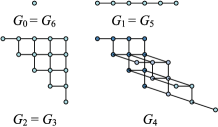
Figure 1: The graphs $G_{k}$ that arise from our construction for the $XY$ interaction on a path of 6 vertices. The hamiltonian $H$ for the $XY$ model is identically equal to the adjacency matrix for the (disconnected) graph $G_{0}\cup G_{1}\cup\cdots\cup G_{6}$, i.e., $H=A(G_{0})\oplus A(G_{1})\oplus\cdots\oplus A(G_{6})$, where $A(G_{k})$ is the adjacency matrix of graph $G_{k}$. Note that $G_{1}=G_{5}$ is equivalent to the path graph.

We now illustrate a final application of our identification of $H_{XY}$ and $H_{\text{Heis}}$ with adjacency matrices and laplacians for the graphs $G_{k}=\bigwedge^{k}(G)$. We consider the $XY$ and Heisenberg models on the graph $K_{N}$, which is the complete graph on $N$ vertices, meaning that every pair of vertices is connected by an edge. In order to solve the $XY$ model on this graph we need to understand the adjacency matrix $A\left(\bigwedge^{k}(K_{N})\right)$. In the case of $K_{N}$ the graph $\bigwedge^{k}(K_{N})$ is easy to describe: the vertices of $\bigwedge^{k}(K_{N})$ are given by $k$-subsets of $V(K_{N})=\{0,1,\ldots,N-1\}$ and two vertices $v_{j}\subset V(K_{N})$ and $v_{k}\subset V(K_{N})$ are connected if and only if they differ, as sets, in only two places, i.e. $|v_{j}\cap v_{k}|=k-1$. This graph is identicalGodsil (1995) to the Johnson graph, denoted $J(N,k)$. The eigenvalues $\lambda_{j}(A(J(N,k)))$, $j=0,1,\ldots,k$, of the adjacency matrix of the Johnson graph are well known and are given by

$$\lambda_{j}(A(J(N,k)))=k(N-k)-j(N+1-j),\quad j=0,1,\ldots,k.$$ (22)

Thus we obtain the complete spectrum for $\sigma(H_{XY})=\{\lambda_{j}(H_{XY})\,|\,j=0,1,\ldots,2^{N}-1\}$:

$$\sigma(H_{XY})=\bigcup_{l=0}^{N}\{\lambda_{j}(J(N,l))\,|\,j=0,\ldots,l\}$$ (23)

We note that the ground-state energy $E_{0}$ for $H_{XY}$ is $E_{0}=-N/2$. Similarly, we observe that the degree of every vertex of the Johnson graph $J(N,k)$ is the same, $d=k(N-k)$, so that the eigenvalues of the Heisenberg model on the complete graph are given by

$$\sigma(H_{\text{Heis}})=\{j(N+1-j)\,|\,j=0,1,\ldots,N\}.$$ (24)

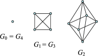
Figure 2: The graphs $G_{k}$ that arise from our construction for the $XY$ interaction on the complete graph $K_{4}$ on four vertices. The hamiltonian $H_{XY}$ for the $XY$ model is identically equal to the adjacency matrix for the (disconnected) graph $G_{0}\cup G_{1}\cup\cdots\cup G_{4}$. Note that $G_{1}=G_{3}=K_{4}$.

While it has been known how to solve the $XY$ model on the path $P_{N}$ using the Jordan-Wigner transformation, the $XY$ and Heisenberg models on the complete graph $K_{N}$ have defied solution using Jordan-Wigner, Bethe ansatz, or any other method.

We note that it is straightforward to include a magnetic field term $BS^{z}$ to our hamiltonians Eq. (1) and Eq. (2) because it leaves the eigenvectors unchanged and only shifts the eigenvalues according to which subspace $\Gamma^{k}$ they are associated with.

Our approach should be compared with the method of Jordan and Wigner which can be used to solve many varieties of $XY$-type model Jordan and Wigner (1928). The Jordan-Wigner transformation utilises exactly the same feature of the $XY$ interaction as our method, i.e. that it conserves total $z$-spin. In addition, the Jordan-Wigner transformation also (implicitly) draws a correspondence between the vector spaces $\Gamma^{k}$ and $\bigwedge^{k}(\mathcal{H}_{G})$. However, the two methods differ when it comes to actually calculating the eigenstates of $H_{XY}$. We solve for the eigenvalues and eigenstates of $H_{XY}$ by understanding the spectral properties of the associated graphs $\bigwedge^{k}G$. The Jordan-Wigner method proceeds by constructing a fermionic hamiltonian $\widetilde{H}_{XY}$ (i.e. a hamiltonian written in terms of fermionic operators $b$ and $b^{\dagger}$) whose action on $\bigwedge^{k}(\mathcal{H}_{G})$ is isomorphic to $H_{XY}$ on $\Gamma^{k}$. This fermionic hamiltonian (which is quadratic) is easily solved via Boguliubov transformation. At this point the eigenvalues and eigenvectors can be constructed trivially. Unfortunately, while the eigenvalues and eigenvectors are simply specified in terms of the fermion operators $b$ and $b^{\dagger}$, the task of inverting the Jordan-Wigner transformation to obtain a representation of the eigenvectors in terms of states in the original basis is a lengthy process.

In contrast, we have explicitly constructed the eigenstates of the $XY$ model on a path. (And, indeed, we can construct the eigenvalues and eigenstates for any graph $G$ for which we can calculate the spectral decomposition of the graphs $\bigwedge^{k}G$.)

In essence, the approach of Jordan and Wigner tries to understand the dynamics of a collection of $k$ noninteracting fermions hopping on a graph. On the other hand, our approach explicitly constructs the configuration space of the $k$ fermions, reducing their dynamics to the dynamics of a single free particle on a (larger) graph.

Perhaps a more intriguing difference between our approach and the Jordan-Wigner method is that our method can also be applied to the Heisenberg interaction. The Jordan-Wigner transformation, when applied to Heisenberg interactions, results in a highly nontrivial nonlocal fermion hamiltonian whose solution is unknown; in the Heisenberg case one must resort to the Bethe ansatz method Bethe (1931). In contrast to this, our method shows that the action of the Heisenberg hamiltonian is the same as the laplacian on the configuration-space graph of the hopping fermions. In this way, as $N\rightarrow\infty$ we expect the statics and dynamics of the Heisenberg and $XY$ models on families of regular graphs will be very similar.

Finally, we point out that our method provides a very simple way to qualitatively understand the quantum dynamics of $XY$ and Heisenberg models on a graph $G$. The idea is that, for intermediate time scales (i.e. time scales up to the order of $N$), and reasonably well-separated spins, one can understand the quantum dynamics as equivalent to the dynamics of a single free particle hopping on the cartesian product graph $G\times G\times\cdots\times G$.

Many future directions suggest themselves at this stage. The most obvious direction is to study the spectral properties of the graph wedge product in detail.

Another promising direction would be to investigate the thermodynamic limit $N\rightarrow\infty$ of $H_{XY}$ and $H_{\text{Heis}}$ on certain families of graphs $G_{N}$, such as the path $P_{N}$, the cycle $C_{N}$, and cartesian products, which have a well-defined continuum limit. In this limit the action of $H_{XY}$ and $H_{\text{Heis}}$ are simply related to the action of the laplacian on the corresponding smooth manifold obeying certain boundary conditions. Even in the mesoscopic limit of large but finite $N$ we should be able to say something about how the spectrum of $H_{XY}$ is related to $H_{\text{Heis}}$, potentially providing a concrete analytical proof of the correctness of the scaling hypotheses at criticality for these models.

A final future direction which presents itself is to investigate the construction of models which have a gap in limit $N\rightarrow\infty$. There are many examples of families of graphs which have a spectral gap in the infinite limit.