Incoherent Noise and Quantum Information Processing

Abstract

Incoherence in the controlled Hamiltonian is an important limitation on the precision of coherent control in quantum information processing. Incoherence can typically be modelled as a distribution of unitary processes arising from slowly varying experimental parameters. We show how it introduces artifacts in quantum process tomography and we explain how the resulting estimate of the superoperator may not be completely positive. We then go on to attack the inverse problem of extracting an effective distribution of unitaries that characterizes the incoherence via a perturbation theory analysis of the superoperator eigenvalue spectra.

I Introduction

One of the biggest challenges in Quantum Information Processing (QIP) is the precise control of quantum systems. Errors in the control are conveniently classified as coherent, decoherent, and incoherent PraviaRFI . Coherent errors are systematic and differ from the desired operation by a unitary operation. Decoherent errors can be expressed by completely positive (CP) superoperators Alicki and can be counteracted by techniques such as Quantum Error Correction (QEC) Shor ; NielsenChuang . An incoherent process can also be described by a completely positive superoperator PraviaRFI ; BoulantEntSwap . The apparent non-unitary behavior of the incoherent process arises due to a distribution over external experimental parameters. The incoherent process is described by a superoperator $S$ acting on Liouville space which can be written, when acting on columnized density matrices $|{\rho}\rangle$ obtained by stacking their columns on top of each other from left to right Havel:03 , as

$$S = \int p(\alpha)\overline{U}(\alpha)\otimes U(\alpha)d\alpha,$$ (1)

where $p(\alpha)$ is a probability density, i.e. the fraction of quantum systems within an ensemble that sees a given $U(\alpha)$ within an interval $d\alpha$, $\int p(\alpha)d\alpha=1$, and $\overline{U}$ denotes the complex conjugate of $U$. This decomposition of a CP map into unitary Kraus operators is sometimes called a random unitary decomposition (RUD) LeungThesis . A RUD exists for an incoherent process, but such a decomposition is sometimes possible even for a very general decoherent process Streater when there is no correspondence between the unitary operators in the decomposition and some actual distribution of associated experimental control parameters $\alpha$. The distinction between the two therefore is practical, and depends primarily on the correlation time of the variation of experimental parameters. If the latter quantity is longer than the inverse of the typical modulation frequency, the process falls into the class of incoherent noise Carr ; Hahn . The point of making this distinction is that, whilst correcting for decoherent errors requires the full power of QEC, in practice incoherent noise effects are often reduced directly through the design of the time-dependence of the control fields. This is possible since the operators underlying the incoherence $U(\alpha)$ are assumed to be time-independent over the length of the expectation value measurement. Common approaches for instance in Nuclear Magnetic Resonance (NMR) include composite and adiabatic pulses Tycko ; Shaka ; Levitt ; Jones ; Pines ; Silver . Furthermore, the work done by Tycko Tycko and Jones Jones2 ; Jones3 on composite pulses finds a great application in QIP since the schemes proposed are universal and therefore work regarless of the input state.

In this paper, we demonstrate how incoherent errors introduce particular limitations to Quantum Process Tomography (QPT) NielsenChuang ; Childs ; BoulantQPT ; Cirac due to the correlations they introduce with an environment in the QPT input states. Prior work has been devoted to the study of the implications of such correlations in the system’s reduced dynamics Buzek ; BuzekErra ; Pechukas . However, to our knowledge they have not explicitly been studied within the context of QPT to show that the method may output non-completely positive (NCP) maps. If the existence or origin of such noise is unknown, it is shown in PraviaRFI by means of explicit examples how one can eventually infer qualitative information, say its symmetry, about the probability distribution underlying the incoherent process from superoperator eigenvalue spectra. In this paper we tackle the inverse problem of extracting an effective probability distribution $p(\alpha)$ representing the incoherent superoperator, given a model for the source of the incoherent noise in the system. Such information is crucial for counteracting the incoherent errors PraviaRFI which, due to their slow variation would otherwise persist during the experiment and quickly accumulate.

II Incoherent Noise and Quantum Process Tomography

QPT measures the experimental map associated with the implementation of a desired quantum operation by passing a complete set of input states through the gate and measuring the corresponding output states (see Fig. 1).

Figure 1: Quantum process tomography method. Starting from thermal equilibrium, a complete set of input states $\{\rho_{in}\}$ are prepared using a set $\{S_{in}\}$ of control sequences. The input and output states are measured using a set of readout pulses $\{U_{ro}\}$ to rotate the density matrix into observable components $\{M_{in}\}$ and $\{M_{out}\}$. The process to be probed represented by a superoperator $S_{exp}$ is then applied to these input states to obtain a corresponding set of output states $\{\rho_{out}\}$. The measured map $S_{obs}$ is then computed by right multiplying the matrix of output states by the inverted one of input states (see text for further details).

This procedure is important for the experimental study of noise processes and for the design of quantum error correcting codes Shor . If incoherent noise is present in the preliminary step of QPT, then the prepared (input) states will be classically correlated with the control parameter $\alpha$ characterizing the incoherence (Eq 1). Furthermore, if the correlation time of the noise in the control parameter is long compared to the coarse-grained time at which the evolution of the system is monitored, then the subsequent dynamics is non-Markovian Cohen-Tannoudji . More specifically, the gate applied to the input state (i.e., the gate being characterized by QPT) will be correlated with the same (slowly-varying) control parameter, and therefore also correlated with the input state to which it is applied. In such cases, the measured dynamics are not guaranteed to be completely positive, and need not correspond to a linear map NielsenChuang ; Buzek ; BuzekErra ; Pechukas .

More generally, any correlations arising from non-Markovian dynamics, whether quantum or classical, can lead to incorrect interpretations of the data obtained from QPT. The “environment” which we assume from the outset is correlated with the system is in general defined by the degrees of freedom that are not part of the system. For example, the different spatial locations of individual qubits in a NMR ensemble, or the bosonic bath producing the fluctuations of the gate charge in a superconducting qubit Weiss .

The basic issues can be seen by exploring the QPT of a spin-$1/2$ system $A$, coupled to a second spin-$1/2$ system $B$ as its environment. Borrowing the example used in Buzek , the initial density matrix of the total system may be written as

$$\rho_{AB}=\frac{1}{4}(I_{AB}+\alpha_{i}\sigma_{i}\otimes I_{B}+\beta_{j}I_{A}\otimes\sigma_{j}+\gamma_{ij}\sigma_{i}\otimes\sigma_{j}),$$ (2)

where $I$ and $\sigma_{i}$ denote the identity and Pauli matrices respectively. The density matrix of the system $A$ is then obtained by tracing over the environment $B$:

$$\rho_{A}=\frac{1}{2}(I_{A}+\alpha_{i}\sigma_{i}).$$ (3)

The dynamics of the whole system $\rho_{AB}$ is a unitary evolution $U_{AB}$, so that the resulting density matrix of $A$ is

$$\rho^{\prime}_{A} = \sum_{\mu}\langle{\mu}|U_{AB}(\rho_{A}\otimes\rho_{B})U_{AB}^{\dagger}|{\mu}\rangle$$

$$+\sum_{\mu}\langle{\mu}|U_{AB}\gamma^{{}^{\prime}}_{ij}\sigma_{i}\otimes\sigma_{j}U_{AB}^{\dagger}|{\mu}\rangle,$$

where $\gamma^{{}^{\prime}}_{ij}=(\gamma_{ij}-\alpha_{i}\beta_{j})/4$ and $\rho_{B}=\mathrm{Tr}_{A}(\rho_{AB})$. Let $\rho_{B}=\sum_{\nu}p_{\nu}|{\nu}\rangle\langle{\nu}|$ and $M_{\mu\nu}=\langle{\mu}|U_{AB}|{\nu}\rangle$. Then the above expression can be reexpressed as

$$\rho^{\prime}_{A} = \sum_{\mu\nu}M_{\mu\nu}\rho_{A}M_{\mu\nu}^{\dagger}$$

$$+\sum_{\mu}\langle{\mu}|U_{AB}\gamma^{{}^{\prime}}_{ij}\sigma_{i}\otimes\sigma_{j}U_{AB}^{\dagger}|{\mu}\rangle$$

The first line therefore corresponds to the Kraus operator sum form Kraus2 of the evolution when initial correlations are not present, while the second line represents the contribution from these correlations. We can easily see that there exist $U_{AB}$, e.g., the swap gate, for which these initial correlations are not observable. In general, however, initial correlations cause the map to be non-linear or NCP.

Within the context of QPT, we now investigate an explicit example of how NCP superoperators can arise. We take a set of $4$ initial density matrices $\rho_{AB}$ such that $\rho_{B}$ is the same in each case, and where the input states $\rho_{A}$ span the Hilbert space of the system $A$ (as required by the QPT procedure)

$$\rho_{AB}^{1} = (I_{AB}+\beta I\otimes\sigma_{z})/4\Rightarrow\rho^{1}_{A,in}=I/2$$

$$\rho_{AB}^{2} = (I_{AB}+\alpha\sigma_{x}\otimes I+\beta I\otimes\sigma_{z}+\gamma\sigma_{x}\otimes\sigma_{z})/4\Rightarrow\rho^{2}_{A,in}=(I+\alpha\sigma_{x})/2$$

$$\rho_{AB}^{3} = (I_{AB}+\alpha\sigma_{y}\otimes I+\beta I\otimes\sigma_{z}+\gamma\sigma_{y}\otimes\sigma_{z})/4\Rightarrow\rho^{3}_{A,in}=(I+\alpha\sigma_{y})/2$$

$$\rho_{AB}^{4} = (I_{AB}+\alpha\sigma_{z}\otimes I+\beta I\otimes\sigma_{z}+\gamma\sigma_{z}\otimes\sigma_{z})/4\Rightarrow\rho^{4}_{A,in}=(I+\alpha\sigma_{z})/2$$

where in each case $\rho_{B}=(I+\beta\sigma_{z})/2$. With the example $U_{AB}=e^{-i\frac{\pi}{4}\sigma_{z}\otimes\sigma_{z}}$, the corresponding $4$ outputs are $\tilde{\rho}_{A}^{1}=I/2$, $\tilde{\rho}_{A}^{2}=(I+\gamma\sigma_{y})/2$, $\tilde{\rho}_{A}^{3}=(I-\gamma\sigma_{x})/2$ and $\tilde{\rho}_{A}^{4}=(I+\alpha\sigma_{z})/2$. We write the density matrices $\rho$ as vectors in Liouville space in the Zeeman basis Havel:03 , which are obtained by first writing the density matrix in the Zeeman basis and then stacking their columns on top of each other from left to right. We refer to the resulting vector simply as the “columnized density matrix”, and will denote it as a ket $|\rho\rangle$. If we set $\alpha=\beta=0.5$ and $\gamma=0.6$, the map $S$ is

$$\begin{aligned} \begin{smallmatrix}&\textsf{Output 1}&\textsf{Output 2}&\textsf{Output 3}&\textsf{Output 4}\end{smallmatrix}\\ \left[\begin{smallmatrix}&0.5~{}~{}~{}~{}&~{}0.5~{}~{}~{}~{}~{}&~{}0.5~{}~{}~{}&~{}0.75\\[12.0pt] &0~{}~{}~{}&~{}0.3i~{}~{}~{}~{}~{}&-0.3~{}~{}~{}&~{}0~{}\\[12.0pt] &0~{}~{}~{}&-0.3i~{}~{}~{}~{}~{}&-0.3~{}~{}~{}&~{}0~{}\\[12.0pt] &0.5~{}~{}&~{}0.5~{}~{}~{}~{}~{}&~{}0.5~{}~{}~{}&~{}~{}0.25\end{smallmatrix}\right]\end{aligned}\begin{aligned} &\begin{smallmatrix}\hskip 21.00005pt\textsf{Input 1}&\hskip 3.5pt\textsf{Input 2}&\hskip 3.5pt\textsf{Input 3}&\hskip 3.5pt\textsf{Input 4}\end{smallmatrix}\\ &=S\cdot\left[\begin{smallmatrix}&0.5~{}~{}~{}~{}&~{}0.5~{}~{}&~{}0.5~{}&~{}0.75\\[12.0pt] &0~{}~{}~{}&~{}0.25~{}~{}&~{}0.25i~{}&~{}0~{}\\[12.0pt] &0~{}~{}~{}&~{}0.25~{}~{}&~{}-0.25i~{}&~{}0~{}\\[12.0pt] &0.5~{}~{}&~{}0.5~{}~{}&~{}0.5~{}&~{}~{}0.25\end{smallmatrix}\right]\end{aligned}~{}\leftrightarrow~{}\begin{aligned} &\\ S~{}=~{}\left[\begin{smallmatrix}&~{}1&0&0&0\\[12.0pt] &0&~{}1.2i&0&0\\[12.0pt] &0&0&~{}-1.2i&0\\[12.0pt] &0&0&0&~{}1\end{smallmatrix}\right]\end{aligned}$$ (4)

which is in general non-linear, since one can no longer predict the output for an arbitrary input state given the action of the gate on these four specific input states alone. However, the map can be considered to act linearly on the system $A$ Hilbert space, i.e. on the linear combinations of input states which contain the right correlations with the environment. For instance, the action of the gate on the input state $(\rho^{2}_{A}+\rho^{3}_{A})/2=(I+\frac{\alpha}{2}(\sigma_{x}+\sigma_{y}))/2$ can be computed by using the above matrix expression if the total input state is $\rho_{AB}=(I_{AB}+\frac{\alpha}{2}(\sigma_{x}+\sigma_{y})\otimes I+\beta I\otimes\sigma_{z}+\frac{\gamma}{2}(\sigma_{x}+\sigma_{y})\otimes\sigma_{z})/4$. This result conveniently allows one to treat the map as linear. If treated as linear, the Choi matrix Choi ${\mathcal{C}}=\sum_{i,j=0}^{N-1}(E_{ij}\otimes I)S(I\otimes E_{ij})$, where $N$ is the dimension of the system’s Hilbert space and $E_{ij}$ is the $N\times N$ elementary matrix (with a ”1” in the $ij-th$ position and zeros elsewhere), corresponding to the superoperator $S$ is not positive semidefinite and consequently $S$ can not be CP Havel:03 .

It is suggested in Havel:03 how the NCP part of the superoperator can be removed, namely, by removing the negative eigenvalues of the Choi matrix and then renormalizing so that the trace is equal to the dimension of the Hilbert space, $N$. We shall call this method CP-filtering. The Choi matrix corresponding to $S$ in (4) has two non-zero eigenvalues $(2.2,-0.2)$. In this example, the CP-filtering procedure replaces the negative eigenvalue by $0$ and then renormalizes the new Choi matrix to trace $N=2$. The CP-filtering method outputs one unitary Kraus operator. On the other hand, if no initial correlations were present, the superoperator would be equal to $S=\mathrm{diag}(1,0.5i,-0.5i,1)$, and the corresponding Choi matrix would have two positive eigenvalues $(0.5,1.5)$, yielding two Kraus operators. This superoperator is therefore completely positive. Unsurprisingly, we thus observe that the superoperator obtained from the CP-filtering procedure is not equal to the superoperator obtained by removing the initial correlations. Therefore, unless the initial correlations are very small, CP-filtering is a fairly uncontrolled procedure, giving CP superoperators that may significantly misrepresent the true quantum dynamics.

We now take the case $\alpha=\beta=\gamma=0.5$ with the same $U_{AB}$ as previously. Although initial correlations are still present, the superoperator obtained by the above QPT method, without CP-filtering, is CP with one Kraus operator. In contrast, if the correlations in the initial states are removed whilst keeping all other things equal, the superoperator obtained is CP with two Kraus operators, not one. So even when initial correlations are present, the superoperator obtained via QPT may be completely positive. Therefore, one cannot rule out the presence of initial correlations merely by the existence of a valid Kraus operator sum form via QPT. Initial correlations can masquerade as CP maps, and in reality the process may not be linear with respect to arbitrary input states.

To summarize, the results of this section are: (i) incoherent errors introduce correlations between the system and the environment in the QPT input states which can persist during the implemented transformation, (ii) these correlations can yield non-completely positive superoperators or non-linear maps, (iii) the CP-filtering method suggested in Havel:03 is not equivalent to removing these initial correlations, and (iiii) initial correlations can masquerade as CP maps which misrepresent what is in reality a non-linear process with respect to the input states. See Table 1 for a summary. This simple analysis explains the apparent NCP behavior measured in experiments reported in BoulantQPT ; WeinsteinQFT . This motivates the need to characterize the incoherent noise, and to provide ways to correctly interpret QPT data. If the noise can be successfully characterized, we may use this information to better counteract the noise in the first place.

	CPF	Corr	CP	Num. Kraus Op.
Ex 1	$\times$	✓	$\times$	-
	✓	✓	✓	1
	$\times$	$\times$	✓	2
Ex 2	$\times$	✓	✓	1
	$\times$	$\times$	✓	2

Table 1: Summary of the two examples given in section II. CPF is abbreviation for CP-Filtering which is an algorithm for converting a non CP superoperator to a CP one. ”Corr” is abbreviation for correlations (between subsystems $A$ and $B$).

III Extracting Probability Distributions from Superoperator Eigenvalue Spectra

By applying a first order perturbation theory analysis of the eigenvalues of superoperators, we now present a method to extract the probability distribution profile $p(\alpha)$ of unitary matrices present in incoherent processes. For an incoherent noise to be refocused Hahn , knowledge about the noise is a priori required. If qualitative information about the inhomogeneity in the Hamiltonian is known, spectroscopic techniques can be used to obtain the missing quantitative information. In the following analysis, we assume that the physical origin of the incoherent noise is unknown or hidden due to the complexity of the system-apparatus interactions, but that a mathematical model is presumed.

As presented in the introduction, an incoherent process implies a random unitary distribution. Incoherent processes are thus unital, which means that the maximally mixed density matrix is left unchanged. A linear, completely positive, trace preserving and unital map is called a doubly stochastic map Alberti . Although a single necessary and sufficient condition for a doubly stochastic map to possess a RUD has not been found to our knowledge, examples of doubly stochastic maps which do not possess a RUD are reported in LeungThesis ; Streater . However, since many decoherent unital processes can be modelled by a stochastic Hamiltonian, i.e. semiclassically, we believe that many instances of decoherent processes can have a RUD. This belief is supported by the following two facts. Any two density operators $(\rho,\rho^{\prime})$ connected by a doubly stochastic map, $\rho^{\prime}=\Lambda(\rho)$, can always be related by a transformation of the form $\rho^{\prime}=\sum_{i}p_{i}U_{i}\rho U_{i}^{\dagger}$, where $\sum_{i}p_{i}=1$ and $\{U_{i}\}$ is a set of unitary operators Alberti . Furthermore, all unital maps for a two-level quantum system always have a RUD Streater .

III.1 Perturbation Theory Analysis of the Eigenvalue Spectra

In what follows, we take examples from NMR Ernst physics where the main source of incoherence comes from Radio Frequency (RF) power inhomogeneity. Due to the spatial extent of the sample, individual spins during the course of a RF field see different powers PraviaRFI and evolve according to different unitary evolutions with different characteristic frequencies. Note that identical spins can have different resonance frequencies due to inhomogeneity in the static magnetic field within the ensemble, which is another source of incoherence. However, as shown in BoulantEntSwap , the non-unitary features arising from this static external field inhomogeneity are usually much smaller than those arising from RF inhomogeneity and will be therefore ignored in this example. Finally while the distribution of RF fields can be easily measured via a nutation experiment on a single spin, the method presented here is quite general and can for instance account for the correlation between multiple sources of incoherence (several RF fields, DC field etc…).

Let $n$ be the number of spin-1/2 particles in the ensemble, and $U_{k}$ denote the unitary operator generated by the RF field in the $k$th frequency interval of the RF amplitude profile. The eigenvalues of the superoperator $S=\bar{U}_{k}\otimes U_{k}$ are products of the eigenvalues of $U_{k}$ with those of $\bar{U}_{k}$. This yields $2^{n}$ eigenvalues that are equal to unity and $(2^{2n-1}-2^{n-1})$ pairs of eigenvalues $(\lambda,\bar{\lambda})$. In general, the eigenvalues of CP superoperators come in conjugate pairs, but only in the case of unitary superoperators do all the eigenvalues lie on the complex unit circle.

The incoherent process resulting from an inhomogeneous distribution of $U_{k}$ processes is given by the superoperator $S=\sum_{k}p_{k}\overline{U}_{k}\otimes U_{k}$, where $p_{k}$ is the fraction of spins that sees the unitary evolution $U_{k}$. The more broadly the $\{p_{k}\}$ are distributed, the larger the degree of inhomogeneity in the evolution, and the more incoherent noise enters into the evolution. Estimates of the actual eigenvalues of $S=\sum_{k}p_{k}\overline{U}_{k}\otimes U_{k}$ will now be obtained using non-degenerate first-order perturbation theory. Because the RF pulses are not perfect, even in the absence of RF field inhomogeneity, we may assume that the unperturbed eigenvalues are generically non-degenerate. The unitary operator $U_{k}$ generated by the RF field acting at position $k$ may be written in exponential form as $U_{k}=e^{-iH_{k}\,t}$ where $H_{k}$ represents the effective Hamiltonian of the evolution over the period $t$ for which the pulse is applied ($\hbar$ has been set equal to $1$). Defining $H_{0}$ to be the unperturbed (and desired) Hamiltonian, the eigenvalues $\phi_{j}$ and eigenstates $|{\phi_{j}}\rangle$ of $H_{0}$ satisfy the eigenvalue equation

$$U_{0}|{\phi_{j}}\rangle=e^{-i\phi_{j}\,t}|{\phi_{j}}\rangle,$$ (5)

where $U_{0}=\exp(-iH_{0}\,t)$. The Hamiltonian of a particular $U_{k}$ is assumed to be a perturbation of the desired, homogeneous Hamiltonian

$$H_{k}=H_{0}+K_{k},$$ (6)

where $K_{k}$ is the perturbation. To first order, the new eigenvalues of $H_{k}$ are

$$\tilde{\phi}_{j,k}=\phi_{j}+\langle{\phi_{j}}|K_{k}|{\phi_{j}}\rangle,$$ (7)

and the corresponding eigenvalues of $U_{k}$ are

$$U_{k}|{\tilde{\phi}_{j,k}}\rangle=e^{-i\tilde{\phi}_{j,k}\,t}|{\tilde{\phi}_{j,k}}\rangle.$$ (8)

To first order, the spectral decomposition of $S$ is

$$S=\sum_{k,m,j}p_{k}\left(e^{i\tilde{\phi}_{m,k}\,t}\overline{|{\phi_{m}}\rangle}\overline{\langle{\phi_{m}}|}\otimes e^{-i\tilde{\phi}_{j,k}\,t}|{\phi_{j}}\rangle\langle{\phi_{j}}|\right)$$ (9)

and the eigenvalues of $S$ are given approximately by

$$\lambda_{jm} = \sum_{k}p_{k}e^{-i(\tilde{\phi}_{j,k}-\,\tilde{\phi}_{m,k})\,t}$$

$$= e^{-i(\phi_{j}-\phi_{m})t}\sum_{k}p_{k}e^{-i\left(\langle{\phi_{j}}|K_{k}|{\phi_{j}}\rangle-\langle{\phi_{m}}|K_{k}|{\phi_{m}}\rangle\right)t}\,.$$

We now imagine the scenario where $K_{k}$ is given by $K_{k}t=\frac{\omega_{k}-\omega_{0}}{\omega_{0}}K$. This result would in fact be exact for one spin on resonance. In this case, $\frac{\omega_{k}-\omega_{0}}{\omega_{0}}$ is the parameter $\alpha$ defined in the introduction (which parameterizes the inhomogeneity) and represents the normalized RF power deviation from the desired power $\omega_{0}$. Defining $\Delta\omega=\frac{\omega_{k}-\omega_{0}}{\omega_{0}}$ and $K_{jm}=\langle{\phi_{j}}|K|{\phi_{j}}\rangle-\langle{\phi_{m}}|K|{\phi_{m}}\rangle$, the previous equation in the continuous limit becomes

$$\lambda_{jm}=e^{-i(\phi_{j}-\phi_{m})t}\int p(\Delta\omega)e^{-iK_{jm}\Delta\omega}d\Delta\omega.$$ (10)

We see in this case that to first order the eigenvalue $\lambda_{jm}$ is just the unperturbed eigenvalue $e^{-i(\phi_{j}-\phi_{m})t}$ times the Fourier transform of the RF distribution profile evaluated at $K_{jm}$. This result demonstrates that the probability distribution profile $p(\Delta\omega)$ of an incoherent process can be determined, within some degree of approximation, from the eigenvalue structure $\{\lambda_{jm}\}$ of an experimental superoperator, given some model for the incoherence $K$. Knowing $K$ would indeed allow one to build the correspondence between $\lambda_{jm}$ and $K_{jm}$, and then to determine $p(\Delta\omega)$ by performing an inverse Fourier transform. Of course, this result holds for general $K$ only when the perturbation is in the first order regime, and when the unperturbed eigenvalues are non-degenerate. But if $K$ approximately commutes with $H_{0}$, then the first-order perturbation in the eigenvalues is close to an exact correction, and the above analysis gives a very accurate description of the incoherent process.

III.2 Recovery of the Profile

We now demonstrate via a numerical example how one can recover the profile $p(\Delta\omega)$ from the eigenvalue spectrum of a measured superoperator. In the theory derived in the previous subsection, $\lambda_{jm}$ is the data, i.e., the eigenvalues from the measured superoperator. A model $K$ is needed for the perturbation, while $\phi_{j}$ and $|{\phi_{j}}\rangle$ are known through the knowledge of $H_{0}$. Formally solving for $p(\Delta\omega)$ from (10),

$$p(\Delta\omega)=\frac{1}{2\pi}\int\lambda_{jm}e^{i(\phi_{j}-\phi_{m})t}\,e^{iK_{jm}\Delta\omega}dK_{jm}.$$ (11)

The different eigenvalues $\lambda_{jm}$ multiplied by $e^{i(\phi_{j}-\phi_{m})t}$ therefore allow us to obtain the complex function of $K_{jm}$ which we shall call $f$, corresponding to the Fourier transform of the distribution profile.

For the numerical demonstration of this technique we take a $3$-qubit system. We choose $H_{0}$ and $K$ such that $|\langle{\phi_{l}}|K|{\phi_{n}}\rangle/(\phi_{l}-\phi_{n})|\simeq 0.1$ for $n\neq l$ and $[H_{0},K]\approx 0$ so that first order perturbation theory can be used Sakurai . We then use a measured RF inhomogeneity profile shown in Fig. 2 to construct the following superoperator acting on Liouville space:

$$S=\sum_{\Delta\omega}p(\Delta\omega)\overline{U}(\Delta\omega)\otimes U(\Delta\omega).$$ (12)

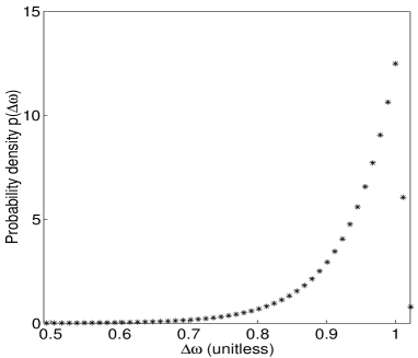
Figure 2: Radio Frequency inhomogeneity profile used to construct the superoperator S ($\int p(\Delta\omega)d\Delta\omega=1$).

Provided with this superoperator, we compute its eigenvalues and plot them on the Argand diagram (see Fig. 3). The perturbation $K$ is such that the first order limit condition is fulfilled, but that the size of its diagonal elements in the $H_{0}$ eigenvectors basis is large enough to generate significant dephasing and attenuation in the eigenvalues. The correspondence between $\lambda_{jm}$ and $K_{jm}$ is needed to recover the distribution profile (11).

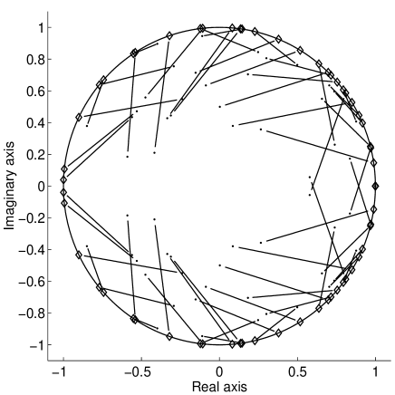
Figure 3: Eigenvalue spectra of the incoherent process $S$ and the desired $S_{0}$. The dots are the eigenvalues of the incoherent superoperator $S$ and the diamonds the ones of the desired unitary superoperator $S_{0}$ (on the unit circle). Also shown is the correspondence between the unperturbed and perturbed eigenvalues. The perturbation $K$ is small enough so that the first order limit condition is fulfilled but large enough to substantially dephase and attenuate the eigenvalues.

The correspondence can be established by first computing $\langle{\overline{\phi_{j}},\phi_{m}}|S|{\overline{\phi_{j}},\phi_{m}}\rangle$, then searching for the eigenvalue of $S$ closest to it. This allows us to make the correspondence between one unperturbed eigenvalue with eigenvector $|{\overline{\phi_{j}},\phi_{m}}\rangle=|{\overline{\phi_{j}}}\rangle\otimes|{\phi_{m}}\rangle$ (obtained from the knowledge of $H_{0}$) and one eigenvalue of $S$. The function $f=\int p(\Delta\omega)e^{-i\Delta\omega K_{jm}}d\Delta\omega$ with respect to $K_{jm}$ can then be constructed. The real and imaginary parts of that function are plotted in Fig. 4.

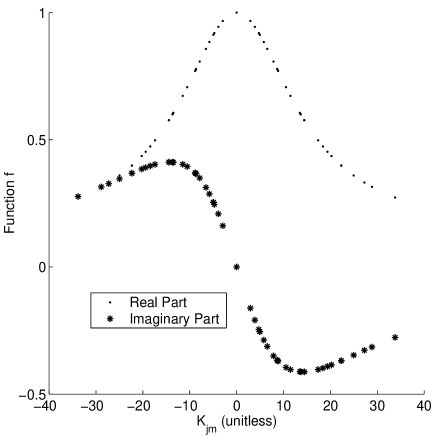
Figure 4: Plot of $f=\int p(\Delta\omega)e^{-i\Delta\omega K_{jm}}$ with respect to $K_{jm}$ (real and imaginary parts). The function is conjugate symmetric with respect to $0$ as expected, so that its inverse Fourier transform, which should be a probability distribution, is real. The point at $K_{jm}=0$ was added to avoid a DC offset in the reciprocal Fourier domain.

Note that we ignore the degenerate points at $f=1$ because they do not provide any information about $p(\Delta\omega)$ other than normalization. The $64$ eigenvalues of the superoperator minus the $8$ degenerate ones equal to $1$ (at $K_{jm}=0$), plus $1$ eigenvalue added at $K_{jm}=0$ to avoid a DC offset in the reciprocal domain, yield a complex function $f$ made of $57$ unequally spaced points. The function $f$ is conjugate symmetric with respect to $0$, which is consistent with the fact that we are supposed to recover a probability distribution, i.e. a real function, after computing the inverse Fourier transform. To perform the inverse Fourier transform of a function sampled at unequally spaced points, we used an algorithm prescribed in MathPaper . The result is shown in Fig .5. The width of the probability distribution and its skewness are recovered to a good extent, the discrepancy being due to the lack of information about the function $f$. It is worth mentioning that with $57$ sample points, the window of $K_{jm}$ values should be large enough to allow low frequency components of the profile to be reliably extracted. If the incoherent perturbations were very small, there will not be as many large values of $K_{jm}$, and therefore less low frequency information would be available.

Figure 5: Inverse Fourier transform of the function plotted in Fig. 4 shown together with points from Fig. 2. The width of the profile in addition to its skewness are recovered to a good extent.

However, the perturbations can be made larger without changing the mathematical model, by simply repeating the control sequence several times, provided other noise mechanisms do not play a significant role. In addition, more points could be used to get a better sampling resolution, with, for instance, a $4$-qubit superoperator yielding $241$ points. One cannot have arbitrarily many points, however, because the correspondence between the eigenvalues of $S$ and those of $S_{0}$ could quickly become impossible to establish unless a very good knowledge of the perturbation $K$ is available. The density of points in the Argand diagram becomes so large that eigenvalues can easily become confused. Here, the $3$-qubit superoperator was enough to recover the essential features of the probability distribution.

If $H_{0}$ is not exactly known, and in fact a constant offset Hamiltonian which is proportional to $K$ is present, then a different function $f$ is obtained :

$$f=\int p(\Delta\omega)e^{-iK_{jm}\Delta\omega}e^{-i\beta K_{jm}}d\Delta\omega,$$ (13)

where $\beta$ is a constant real number. Taking the inverse Fourier transform of $f$ would reveal a distribution $p(\Delta\omega)$ centered around $\beta$ rather than $0$, indicating that $H_{0}+\beta K$ is in fact the unperturbed Hamiltonian. Perfect knowledge about $H_{0}$ as a result is not required provided the offset is approximately proportional to $K$.

It is important for this method to work that the model $K$ chosen a priori is a reasonably faithful one, and that it approximately commutes with $H_{0}$. This ensures that the applied first-order perturbation theory is valid. In the extreme case, in which $K$ anticommutes with $H_{0}$, $\langle{\phi_{j}}|K|{\phi_{j}}\rangle=0~{}\forall j$ and no “data” would be available for analysis. It is also worth mentioning that this method is, needless to say, not scalable. However, in many instances, as in NMR, the inhomogeneity features are apparatus dependent, so that reasonably small physical systems can be used to probe them. The scalability of the method is not necessarily a requirement. The distribution of some control parameters, once obtained, can be valuable in designing robust control sequences PraviaRFI for larger and more complex systems.

IV Conclusion

Here we reviewed that when incoherence is present during the preparation of the input states for QPT, the resulting correlations between the system and the ”environment” can play an important role on the subsequent system’s dynamics. The map obtained by right multiplying the matrix of output states by the inversion of the matrix of input states still has a meaning, but a correct interpretation of the measured data (or transformation) requires an analysis of the incoherence effects affecting the tomographic procedure. In particular, the measured map needs not be CP. If quantitative information is missing, our perturbation theory analysis of superoperator eigenvalue spectra can be used to determine an effective distribution of unitaries characterizing the process, provided a good mathematical model is available. While this requires a significant effort to measure a 3-qubit superoperator, it is certainly feasible within present experimental capabilities. Lastly, the knowledge of the distribution of control parameters should finally allow us to design more efficient control sequences aimed at counteracting these deleterious effects.

V Acknowledgements

This work was supported by ARO, DARPA, NSF and the Cambridge-MIT institute. Correspondence and requests for materials should be addressed to D. G. Cory (e-mail: dcory@mit.edu). We thank Marcos Saraceno for valuable discussions.

References

- (1) M. Pravia, N. Boulant, J. Emerson, E. Fortunato, A. Farid, T. F. Havel, and D. G. Cory, J. Chem. Phys. 119, 9993 (2003).
- (2) R. Alicki and M. Fannes, Quantum Dynamical Systems (Oxford University Press, Oxford, 2001).
- (3) P. Shor, Phys. Rev. A 52, 2493 (1995) ; A. M. Steane, Phys. Rev. Lett. 77, 793 (1996) ; J. Preskill, Proc. Roy. Soc. London A 454, 385 (1998).
- (4) M. A. Nielsen and I. L. Chuang, Quantum Computation and Quantum Information (Cambridge University Press, Cambridge, 2001).
- (5) N. Boulant, K. Edmonds, J. Yang, M. Pravia, and D. G. Cory, Phys. Rev. A 68, 032305 (2003).
- (6) T. F. Havel, J. Math. Phys. 44, 534 (2003).
- (7) D. Leung, Towards Robust Computation, Ph.D. thesis, Stanford University (2000).
- (8) L. J. Landau, and R. F. Streater, Lin. Alg. Appl. 193, 107-127 (1993).
- (9) H. Y. Carr and E. M. Purcell, Phys. Rev. 93, 749 (1954).
- (10) E. L. Hahn, Phys. Rev. 80, 580 (1950).
- (11) R. Tycko, Phys. Rev. Lett. 51, 775 (1983).
- (12) A. Shaka and R. Freeman, J. Magn. Reson. (1969-1992) 55, 487 (1983).
- (13) M. Levitt, Prog. Nucl. Magn. Reson. Spectrosc. 18, 61 (1986).
- (14) H. K. Cummins, G. Llewellyn, and J. Jones, Phys. Rev. A 67, 042308 (2003).
- (15) J. Baum, R. Tycko, and A. Pines, Phys. Rev. A 32, 3435 (1985).
- (16) M. S. Silver, R. I. Joseph, and D. I. Hoult, Phys. Rev. A 31, 2753 (1985).
- (17) J. A. Jones, quant-ph/0301019.
- (18) H. K. Cummins, and J. Jones, New J. Phys. 2, 6.1-6.12 (2000).
- (19) A. M. Childs, I. L. Chuang, and D. W. Leung, Phys. Rev. A 64, 012314 (2001).
- (20) N. Boulant, T. F. Havel, M. A. Pravia, and D. G. Cory, Phys. Rev. A 67, 042322 (2003).
- (21) J. F. Poyatos, J. I. Cirac, and P. Zoller, Phys. Rev. Lett. 78, 390 (1997).
- (22) P. telmachovi, and V. Buek, Phys. Rev. A 64, 062106 (2001).
- (23) P. telmachovi, and V. Buek, Phys. Rev. A 67, 029902 (2003).
- (24) P. Pechukas, Phys. Rev. Lett. 73, 1060 (1994).
- (25) C. Cohen-Tannoudji, J. Dupont-Roc and G. Grynberg, Atom-Photon Interactions, Basic Processes and Applications (John Wiley & Sons, New York, 1998).
- (26) U. Weiss, Quantum Dissipative Systems, Volume 2 of Series in Modern Condensed Matter Physics (World Scientific, Singapore, 1998).
- (27) K. Kraus, Ann. Phys. 64, 311 (1971).
- (28) M. D. Choi, Lin. Alg. Appl. 10, 285 (1975).
- (29) Y. Weinstein, T. F. Havel, J. Emerson, N. Boulant, M. Saraceno, S. Lloyd and D. G. Cory, in press in J. Chem. Phys.
- (30) P. M. Alberti, and A. Uhlmann, Stochasticity and Partial Order: Doubly Stochastic Maps and Unitary Mixing (Dordrecht, Boston, 1982).
- (31) R. R. Ernst, G. Bodenhausen, and A. Wokaun, Principles of Nuclear Magnetic Resonance in One and Two Dimensions (Oxford University Press, Oxford, 1994).
- (32) J. J. Sakurai, Modern Quantum Mechanics (Addison-Wesley, New York, 1994).
- (33) A. Dutt and V. Rokhlin, Fast Fourier Transforms for nonequispaced data, Siam J. Sci. Comput. 14(6) 1368–1393 (1993).