Robustness of non-abelian holonomic quantum gates against parametric noise

Abstract

We present a numerical study of the robustness of a specific class of non-abelian holonomic quantum gates . We take into account the parametric noise due to stochastic fluctuations of the control fields which drive the time-dependent Hamiltonian along an adiabatic loop. The performance estimator used is the state fidelity between noiseless and noisy holonomic gates. We carry over our analysis with different correlation times and we find out that noisy holonomic gates seem to be close to the noiseless ones for ’short’ and ’long’ noise correlation times. This result can be interpreted as a consequence of to the geometric nature of the holonomic operator. Our simulation have been performed by using parameters relevant to the excitonic proposal for implementation of holonomic quantum computation [P. Solinas et al. Phys. Rev. B 67, 121307 (2003)]

I Introduction

The use of uniquely quantum phenomena to process information has led to surprising results in quantum key distributions crypto , information transfer protocols teleportation and computation algos . From the point of view of the actual implementation of these theoretical protocols a main challenge is posed by the fact that generically quantum states are very delicate objects quite difficult to control with the required accuracy. The interaction with the many degree of freedom of the environment causes the loss of information (decoherence) and moreover errors in processing the information lead to a wrong output state (control errors). The first problem has been extensively studied over the past few years and a few ways to overcome it have been proposed and experimentally realized. These strategies include error avoiding error_avoiding , error correcting strategies error_correcting and decoupling techniques bang-bang .

A new approach called topological quantum computation has been argued to be able to effectively solve both of them and open new ways to inherently robust quantum computation topological . Information is encoded in topological degrees of freedom of a system which are not sensitive to the local environment-noise effects and then are robust against decoherence tns . Unfortunately to the date, no simple feasible physical system has been identified to this aim; in fact, the systems proposed are usually complicated many-particle ones living over a macroscopic non-trivial structure (e.g. torus or cylinder topology). On the other hand, we can develop topological information processing, where the operator used depends on topological controls and then are robust against a the unwanted fluctuations of the driving fields. In this case, a important intermediate step is the geometrical quantum computation and particularly promising is the fully-geometrical approach called Holonomic Quantum Computation (HQC) HQC .

At variance with topological information processing, for geometrical QC several implementation proposals have been made; indeed the holonomic structure shows up in a variety of quantum systems, both in its Abelian (Berry) abelian and non-Abelian version HQC_proposal ; duan ; paper1 ; long_pap . For this reason interest around HQC has recently growth leading also to proposals in which the adiabatic request can be relaxed and for implementing geometrical non-adiabatic quantum computation non_adiabatic . One of the apparent advantages of HQC is that the gating time for holonomic gates does not depends on the logical operator applied but only on the adiabatic request; then HQC may lead to a new approach to implement complex operators difficult to construct with the standard dynamical gates (as discussed in long_pap ). In view of its geometric nature i.e., dependence on areas spanned by loops in the control parameter manifold, HQC has been suggested to be robust against some class of errors preskill ; ellinas . Nevertheless thorough studies aimed to address this important issue are still relatively few and certainly not exhaustive HQC_noise .

In this paper we will deal with the noise due to imprecise control of the system parameters during the evolution. This error source will be referred to as parametric noise. We will show that the fidelity of the holonomic gates displays three regimes, depending on the ratio between the adiabatic time and the noise correlation time. This results can be understood in view of the geometrical dependence of the holonomic operator. We will study in detail the class of holonomic gate proposed in paper1 in which the physical system are semiconductor quantum dots, the logical qubits are excitonic quantum state controlled by ultrafast lasers.

In section II, after a brief review of the holonomic approach, we describe the system used and the logical gate studied; moreover, it is discussed how we model the noise in the control parameters. In Sec. III we give a description of our simulations and show the results with different kind of noise processes for two single qubit gates and for a two qubit gate. A comparison with dynamical gates subject to the same noise is given too. Section IV contains the conclusions.

II Holonomic quantum gates with parametric noise

Let us consider a family $\mathcal{F}$ of isodegenerate Hamiltonians $H(\lambda)$ depending on $m$ dynamically controllable parameters $\lambda$, in the HQC approach HQC one encodes the information in a $n-$fold degenerate eigenspace $\mathcal{E}$ of an Hamiltonian $H(\lambda_{0})$. Varying the $\lambda$’s and driving adiabatically $H(\lambda)$ along a loop in the $\lambda$ manifold we produce a non-trivial transformation of the initial state $|\psi_{0}\rangle\rightarrow U|\psi_{0}\rangle$. These transformations, known as holonomies, are the generalization of Berry’s phase and can be computed in terms of the Wilczek-Zee gauge connection W-Z : $U(C)={\bf P}exp(\oint_{C}A)$ where $C$ is the loop in the parameter space and $A=\sum_{\mu=1}^{m}A_{\mu}d\lambda_{\mu}$ is the $u(n)-$valued connection. If $|D_{i}(\lambda)\rangle$ ($i=1,...,n$) are the instantaneous eigenstates of $H(\lambda)$, the connection is $(A_{\mu})_{\alpha\beta}=\langle D_{\alpha}|{\partial}/{\partial\Omega^{\mu}}|D_{\beta}\rangle$ ($\alpha$, $\beta=1,...,n$). The set of holonomies associate with a given connection is known to be a subgroup of the group of all possible $n$-dimensional unitary transformations; when the dimension of this holonomy group and coincides with the dimension of $U(n)$ one is able to perform universal quantum computation with holonomies HQC .

For concreteness in this paper we will focus on the class of holonomic quantum gates analyzed in paper1 ; long_pap . Logical qubits are given by polarized excitonic states controlled by femtosecond laser pulses. The parameters we have used in performing our simulations are those relevant to this specific kind of physical systems.

First we concentrate to one-qubit gates. Despite this might look at first as major limitation, we observe that, as far as the holonomic structure is concerned, the two-qubit gates are very similar. So we expect that most of the results we are going to present here e.g., the existence of separate regimes, should, to a large extent, hold true for two-qubit gates too.

The time-dependent interaction Hamiltonian in the interaction picture is

$$H_{int} = -\hbar(\Omega_{+}|E^{+}_{L}\rangle+\Omega_{-}|E^{-}_{L}\rangle+\Omega_{0}|E^{0}_{L}\rangle)\langle G|$$ (1)

$$+ h.c.$$

where $|E^{i}_{L}\rangle$ ($i=+,-,0$) are the polarized excitonic states (two logical and one ancilla) and $|G\rangle$ is the ground state (absence of exciton). This Hamiltonian family admits two dark states i.e., $H_{int}(\Omega)|D_{i}(\Omega)\rangle=0,\,(i=1,2).$ This two-fold degenerate manifold represent contains our encoded logical qubit: $|0\rangle_{L}:=|E^{+}_{L}\rangle,\;|1\rangle_{L}:=|E^{-}_{L}\rangle.$ In Refs. duan ; paper1 it has been shown that the Wilczek-Zee connection associated to the Hamiltonian family (1) allows to construct universal one-qubit gates. These are realized by giving an explicit prescription for driving the control parameter $\Omega$’s along suitable adiabatic loops.

We suppose now to add to the control $\Omega$-field a ’small’ noise which perturbs our trajectory on the control manifold. We test the robustness of the geometrical mixing single-qubit gate proposed in Ref. paper1 . To obtain this gate, we made the following loop in the parameter space : $\Omega_{-}(t)=\Omega~{}\sin\theta\cos\varphi$, $\Omega_{+}(t)=\Omega~{}\sin\theta\sin\varphi$ and $\Omega_{0}(t)=\Omega~{}\cos\theta$ (where the $\Omega$ parameters is fixed and the $\theta(t)$ and $\varphi(t)$ are time dependent) and the holonomic operator obtained at the end of the loop is $U=e^{i\phi\sigma_{y}}$, (where $i\sigma_{y}=|E^{+}_{L}\rangle\langle E^{-}_{L}|-|E^{-}_{L}\rangle\langle E^{+}_{L}|$). The geometrical parameter $\phi=\oint\sin\theta d\theta d\varphi$ is the solid angle spanned by the parameter vector $\vec{\Omega}=(\Omega_{+},\Omega_{-},\Omega_{0})$ on the parameter manifold (sphere). Changing the relation between $\theta$ and $\varphi$ we change the loop and then the value of $\phi$. We choose a loop in order to obtain $\phi=\pi/2$ and $U=exp(i\pi\sigma_{y}/2)=|E^{+}_{L}\rangle\langle E^{-}_{L}|-|E^{-}_{L}\rangle\langle E^{+}_{L}|$.

The logical operator $U$ depends only on geometrical parameters (i.e. solid angle swept on the parameters manifold), every perturbation that changes the trajectory in the control manifold changes the operator leading to computational errors. This notwithstanding, the perturbations leaving (almost) unchanged this angle will not affect the holonomic operator. Then we expect that even strong fluctuations - provided their time scale is sufficiently fast - average out, leaving in this way the angle unchanged and thus not affecting the computation.

The control parameters are the intensities and the phases of the lasers (since we suppose to be in resonant condition, we have fixed frequencies) perturbed by external noise (one for the phases and one for the intensities). To clarify which of these mainly affects the gate operation, first we separate the two types of errors (intensity and phase fluctuations) and then we apply both of them.

We use a straightforward model for the noise : we extract a random number from a probability distribution, we add a constant noisy field for the time $T_{n}$ to the evolving control field, then we extract another random number and so on. To simplify the simulations we choose $T_{n}$ in such a way that $T_{ad}$ is a multiple of $T_{n}$ ($T_{ad}=n_{r}T_{n}$). The fundamental parameter is the noise time $T_{n}$  that is the lapse of time of each random extraction; i.e. it represents the time scale of each random fluctuation.

Figure 1: Fidelity for holonomic gate with $\Omega^{-1}=50~{}fs$, $T_{ad}=7.5~{}ps$ ($\Omega~{}T_{ad}=150$) and $\delta\Omega=0.1\Omega$. (A) Slowly varying fluctuations and (B) fast varying fluctuations.

For the ’intensity’ noise we modify only the value of the Rabi frequencies $\Omega$. We have three lasers turned on and we suppose they have independent fluctuations $\delta\Omega_{i}$ (i.e. every $T_{n}$  we extract three random numbers). The evolution on the control manifold is described by:

$$\left\{\begin{array}[]{lcl}\Omega_{-}(t)&=&\Omega~{}\sin\theta\cos\varphi+\delta\Omega_{-}(t)\\ \Omega_{+}(t)&=&\Omega~{}\sin\theta\sin\varphi+\delta\Omega_{+}(t)\\ \Omega_{0}(t)&=&\Omega~{}\cos\theta+\delta\Omega_{0}(t)\end{array}\right.$$

In this case, the Rabi frequencies remain real parameters, but, if we introduce a ’phase’ noise ($\Omega_{j}\rightarrow e^{i\xi_{j}}\Omega_{j}$), they acquire an imaginary part. The random numbers are taken as before and the evolution in the control manifold is:

Figure 2: Loop in the parameter space for the holonomic gate with (solid line) and without noise (dashed line). With extraction of 2 ($T_{n}=T_{ad}/2$) (A) and 70 random numbers ($T_{n}=T_{ad}/70$) (B). The sphere radius is normalized to $\Omega=1$.

$$\left\{\begin{array}[]{lcl}\Omega_{-}(t)&=&e^{i\xi_{-}}~{}\Omega~{}\sin\theta\cos\varphi\\ \Omega_{+}(t)&=&e^{i\xi_{+}}~{}\Omega~{}\sin\theta\sin\varphi\\ \Omega_{0}(t)&=&e^{i\xi_{0}}~{}\Omega~{}\cos\theta\end{array}\right.$$

The most general and complicated situation is when both ’intensity’ and ’phase’ noise are present.

III Simulations

For all the simulation we choose the parameters used in Refs. paper1 ; long_pap which satisfy the adiabatic condition : $\Omega=0.02$ fs^-1, $T_{ad}=7.5$ ps and $\Omega~{}T_{ad}=150$. The probability distribution for the noise is a Gaussian with zero mean and $<\sigma>=<\frac{\delta\Omega}{\Omega}>=0.1$ where $\delta\Omega$ is the fluctuation of the Rabi frequency. Though this value is far below the experimental control, we use it to understand the robustness of holonomic gates against strong perturbations.

Once the evolution of the state with the noise has been computed, we must compare it with the ideal one in which the noise is absent. In order to make such a comparison quantitative we introduce the fidelity

$$\mathcal{F}=\sqrt{\langle\psi^{id}_{out}|\rho_{out}|\psi^{id}_{out}\rangle}$$ (2)

where $|\psi^{id}_{out}\rangle$ is the final state without noise and $\rho_{out}$ is the density matrix of associated to the noisy final state. In our case the evolution is unitary, then $\rho_{out}=|\psi_{out}^{noise}\rangle\langle\psi_{out}^{noise}|$ and the fidelity reduce to be a scalar product between the noisy and the ideal state. To eliminate the dependence of (2) on the initial states we make a sampling of the initial state space and then average the results. Even if we have a four dimensional working space, the initial state space has dimension two; in fact, in the ideal gates (once satisfied the adiabatic condition) we always start and end in a superposition of the logical states $|E^{+}_{L}\rangle-|E^{-}_{L}\rangle$. This simplifies the sampling procedure because we can take the Bloch sphere as sampling space. We sample the Bloch sphere with $18$ states sample and for each of them calculate the fidelity. Fixed the random numbers extracted during the evolution (i.e. fixed $T_{n}$), we have also to take into account the dependence from the series of the random number extracted. For every sampled state we make five different realization with different extracted random numbers and calculate the average fidelity for the particular initial state. Finally, we make the average fidelity for all the sampled states to obtain the fidelity of our gate for a fixed $T_{n}$.

In the Figures presented here on the $y$  axis is plotted the fidelity and on the $x$ axis is plotted the number of extractions (that is the the ratio $T_{ad}/T_{n}$ between the adiabatic and noise time).

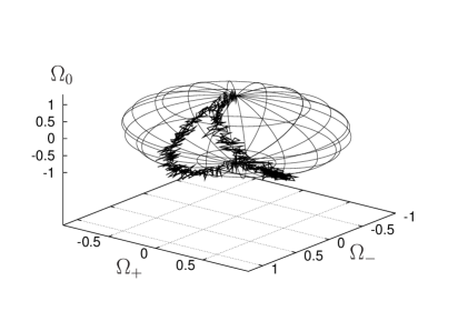
Figure 3: Loop in the parameter space for the holonomic gate with noise and the extraction of 5000 random numbers ($T_{n}=T_{ad}/5000$). The sphere radius is normalized to $\Omega=1$.

In Figures 1 we report the simulated evolution for two regimes of noise. In fig. 1 (A) we plot the fidelity when we extract up to $100$ random numbers during the evolution ($T_{ad}/100\leq T_{n}\leq T_{ad}$). Up to $30$ random numbers the average fidelity is $0.875$, while it decreases up to a minimum of about $0.5$ (with total average of $0.632$) if we extract more random numbers.

A possible interpretation of this effect can be given looking at Figure 2 where we show the evolution on the parameter sphere. In figure 2 (A) $n_{r}=2$  ($T_{n}=T_{ad}/2$) and we change the noise field twice during the evolution. Despite the intense noise, the shape of the loop is still clearly visible, it is simply shifted with respect to the ideal one. The value of the resulting solid angle swept is near to the ideal one. In figure 2 (B) we extract $n_{r}=70$  random extractions during the adiabatic evolution ($T_{n}=T_{ad}/70$). The fluctuations are too intense and too few to cancel out then, as we expected, the solid angles, swept, respectively during the ideal and the noisy loops, are different. This can explain the result in figure 1 (A).

As stated before, even if we have strong fluctuations, we expect that if we extract many random numbers the noise in average does not affect the solid angle and leave the holonomic operator unaffected. This is what seems to be confirmed by the simulations illustrated in Figure 1 (B) where we extract from $50$ to $5000$ random numbers. The fidelity increases and it is even better of those in figure 1 (A); the average fidelity is $0.918$ but it increases to $0.956$ if take into account the values from $1000$ to $5000$ random extractions. The relative loop in the parameter space is shown in figure (3) where we extract $5000$ random numbers during the evolution: the fluctuations have $\delta\Omega=0.1~{}\Omega$ but are so quick that cancel out.

From these simulations it is evident that we have three regimes in our model which can be explained as the sign of the geometrical dependence of the holonomic operator:

Figure 4: Fidelity for small perturbations $\delta\Omega=0.01\Omega$. Parameters as in figure 1.

Figure 5: Fidelity for the ’phase’ noise. Parameters as in figure 1.

• Slowly varying random fluctuations ($T_{ad}/T_{n}\approx 1$): the loop basically maintains its shape and it is simply shifted. This situation does not affect the gate too much.

• Intermediate regime ($50\leq T_{ad}/T_{n}\leq 100$): the intense fluctuations badly modify modify the loop shape and alter the gate operator.

• Fast varying random fluctuations ($T_{ad}/T_{n}\gg 1$): the fluctuations effectively cancel out and do not change the operator.

These geometrical features are independent from the ratio $\delta\Omega/\Omega$ and persist even for small values of the fluctuation $\delta\Omega$. If we decrease the intensity of the noise our adiabatic gate improves as shown in Figures (4) where, with the same parameters (i.e. Rabi frequency and adiabatic time), we choose $\delta\Omega=0.01\Omega$. We note that the fidelity increases but the features are the same of the previous simulations (i.e. three regimes).

Figure 6: Fidelity for holonomic gates when the system is subject to ’intensity’ and ’phase’ noise. Parameters as in figure 1.

In Figure (5) the noise is applied only to the phase of the control field with the same adiabatic parameters of the previous simulations. Since the way of producing the operator is always the same (i.e. loop in the parameter space with a noise), we expect that the effects of noise are the same of those for ’intensity’ noise. This can be clearly seen in figures (5) where we find the same features of the previous plots. The fidelity is much better respect to ’intensity’ noise and we can say the the ’phase’ noise does not affect our gate.

We finally discuss the case of both intensity and phase noise (Figure 6). As we expect, the main part of the error is given by the intensity noise . The three regimes, discussed previously, are evident also in this case.

In Figures (7) we show the population of the non-logical states ($|G\rangle$ and $|E^{0}_{L}\rangle$) at the end of the gate application as function of $T_{ad}/T_{n}$. In an ideal adiabatic gate (for $T_{ad}\rightarrow\infty$) these states are not populated. In Figure (7) (A) these populations increase with the $T_{ad}/T_{n}$ ratio due to the strong and fast fluctuations of the Rabi frequencies which perturb the Hamiltonian. For very fast varying fluctuations (Figure 7 (B)) the undesired populations decrease because of cancellation effects. From this analysis we can say that for slowly and fast varying random fields (i.e. the two extreme regimes) we remain in the logical computational space.

Figure 7: Population of the non-logical sates $|G\rangle$ and $|E^{0}_{L}\rangle$ after the holonomic gate application when the system is subject to ’intensity’. Parameters as in figure 1.

We wish to compare this holonomic gate with a standard dynamical gate, the latter one being characterized by the same unitary operator of the holonomic one and having different (typically shorter) gating time (the time need for the application of the gate). In our system this means to consider as logical states $|G\rangle=|0\rangle$ and $|E^{i}_{L}\rangle=|1\rangle$ and apply a $\pi-$pulse laser sequence to produce a transition $|G\rangle\leftrightarrow|E^{i}_{L}\rangle$.

Figure 8: Comparison between holonomic (solid line) and dynamical (dashed line) gates with (A) $\delta\Omega=0.1\Omega$  and (B) with $\delta\Omega=0.01\Omega$ . On the top $T_{ad}/T_{n}$ for the holonomic gate and on the bottom $T_{dyn}/T_{n}$ for dynamical gates are reported.

We made similar simulations for dynamical gate with the same parameter ($\Omega=0.02$ fs^-1) and with the same noise.

In Figures (8) we make a comparison between holonomic (solid line) and dynamical gates (dashed line) subject to the same intensity and phase noise. The comparison is not direct since the gating times are different. This means that the ratios $T_{ad}/T_{n}$ and $T_{dyn}/T_{n}$ are different for adiabatic and dynamical gates. To compare the effect of the gate subject to the same noisy field (i.e. with the same noise time $T_{n}$), we have to take into account that the dynamical gates, in our model, are about 100 times faster than the adiabatic ones (see Refs. paper1 ; long_pap ). This means that if during the adiabatic evolution the noise changes $n_{r}^{ad}=T_{ad}/T_{n}$ times, for the dynamical gates it changes only $n_{r}^{dyn}=T_{ad}/(100~{}T_{n})$ times (if for the dynamical noise $n_{r}^{dyn}<1$, it changes only once). In other words, if for dynamical gate we extract $n_{r}^{dyn}$ random numbers during the evolution, for the holonomic gate we extract $n_{r}^{ad}=100~{}n_{r}^{dyn}$ random numbers. This means that to compare the fidelities we have to look in the fast varying fluctuating noise ($T_{ad}/T_{n}\gg 1$) region of the previous figures.

Figure 9: Fidelity for the single qubit phase shift gate with to intensity noise. The parameter are the same of figure 1

.

Figure 10: Fidelity for the two qubit phase shift gate with to intensity noise. Parameters are : $\delta=5$ meV, $|\Omega_{i}|=\delta/15$ and $T_{ad}=0.8$ ns.

For this reason in Figures 8 (A) and (B) we put two different scales for the adiabatic ($T_{ad}/T_{n}$) and dynamical ($T_{dyn}/T_{n}$) gates and the plots have been rescaled taking into account for the different gating time.

Numerical simulations in Fig. 8 show that the performance of holonomic gates and dynamical gates are comparable in the region where the first ones are reliable; that when $T_{ad}/T_{n}\gg 1$ (see discussion above).

Both dynamical and holonomic gates can be further improved. Since the dynamical gates are not subject to adiabatic constraints, we can choose different parameters in order to minimize the effect of the noise but this can affect the gating time.

For holonomic gates, given a noise with fixed correlation noise time $T_{n}$, we can try to change adiabatic time in order to modify the $T_{ad}/T_{n}$ ratio. This should allow us to fall in a ’good’ regime i.e. fast or slowly varying fluctuations. Decreasing adiabatic time to get in the small $T_{ad}/T_{n}$ region can produce new errors due to the lack of adiabaticity during the evolution and then it must be treat carefully. Increasing the adiabatic time to enter in the region of great $T_{ad}/T_{n}$ leads both to a better precision in the adiabatic gates and to the cancellation of noisy fluctuations but gives longer gating times.

To complete the set of universal quantum gates, we need another single qubit gate and a two qubit gate.

In the first case, we apply an intensity noise to the phase gate presented in Ref. paper1 with $\Omega_{-}=0$, $\Omega_{+}=-\Omega\sin(\theta/2)~{}e^{i\varphi}$ and $\Omega_{0}=\Omega\cos(\theta/2)$. The holonomic operator is $U=e^{i\phi|E^{+}\rangle\langle E^{+}|}$ where $\phi=\frac{1}{2}\oint\sin\theta d\theta d\varphi$. The results are shown in Figures (9) and the structures discussed above are evident.

Finally, in Figures (10) we present the simulations of the phase shift two qubit gate in Ref. paper1 with an intensity noise. In this case we use two exciton states ($|E^{i}_{L}E^{j}_{L}\rangle$ and $|GG\rangle$) and a two photon interaction Hamiltonin similar in structure to (1) but with Rabi frequency $\Omega_{eff}=2\hbar\Omega^{2}/\delta$ (where $\delta$ is the laser detuning we need to avoid single photon transition and create two exciton states).

In Figure (10) (A) where the second regime (where the fidelity decreases) is present but less evident and seems to be compressed in the slowly varying random fluctuations zone ($10\leq T_{ad}/T_{n}\leq 30$); for great $T_{ad}/T_{n}$ ratio the fidelity decisively increases as in the previous figures (Figure (10) (B)). Moreover, we note that the fidelity between the adiabatic final states with and without noise is high and close to $1$ even if we have chosen the adiabatic parameter ($\Omega_{eff}~{}T$) smaller than the one used for single qubit gates. These can be explained as consequence of the fact that in the imperfect adiabatic evolution unwanted states gets populated. On the other hand the effect of the fluctuating noise is to induce undesired transition as well. These two effects are superposed and with smaller adiabatic parameter the effect of the noise seems to be less important.

IV Conclusions

We numerically studied the robustness of a non-abelian holonomic quantum gate against stochastic errors in control parameters. The robustness of logical gates show three regimes upon the variations of the noise correlation time $T_{n}$. A possible interpretation of these regimes can be given on the basis of the the geometric (i.e. solid angle swept in the parameter space) dependence of the holonomic operator. For fast random varying fluctuations we have a good robustness of the holonomic gate since, as argued in other papers preskill ; ellinas , the fluctuations during the loop tend to cancel out. For random varying fluctuations in the intermediate regime the holonomic gates are significantly corrupted because the fluctuations strongly deform the parameter loop. For slowly random varying fluctuations the performance improves again. This fact is not surprising as it may seem, indeed the loop in the parameter space turns out in this case to be simply is shifted rather than deformed; then similar solid angles are swept. Our analysis suggests that the main noise source is given by fluctuations in the intensity of the control parameters whereas the phase fluctuations do not seem to sizeably affect the gate studied. The effect of the noise decreases with the variance of the intensity of the fluctuations and for $\delta\Omega/\Omega=0.01$ we have average fidelity close to $1$. A first comparison shows that holonomic and dynamical gates have comparable performance in the $T_{ad}/T_{n}\gg 1$ region.

We performed similar simulations for two single qubit gates and for a two qubit gate in order to complete the set of universal quantum gates. For the single qubit gates we obtain similar results. For the two qubit gate the three regimes descibed above are present but less evident.

We believe that our analysis and conclusions should be extended rather easily to different sort of system proposed for HQC: for example, it definitely extends to the model proposed in ref. duan since the involved holonomic structure is isomorphic to the one here analyzed. The general features of our results should hold also more general situations, since they apparently do not rely on the detailed features of Hamiltonian (1), rather on the general structure of holonomic computations. A related, though logically distinct, issue is the robustness of HQC against environmental decoherence florian . This is clearly an important subject to be addressed in future investigations.

P.Z. gratefully acknowledges financial support by Cambridge-MIT Institute Limited and by the European Union project TOPQIP (Contract IST-2001-39215)

References

- (1) C.H. Bennett and G. Brassard Proceedings of IEEE International Conference on Computers, Systems and Signal Processing 175-179, IEEE, New York, 1984. C. H. Bennett Phys. Rev. Lett. 68(21), 3121, 1992.
- (2) C.H. Bennett G. Brassard, C. Crepeau, R. Jozsa, A. Peres, and W. K. Wootters Phys. Rev. Lett. 70, 1895, 1993.
- (3) P.W. Shor Proceeding of 35th Annual symposium on foundation of Computer Science. (IEEE Computer Society Press, Los Alamitos, CA, 1994). L.K. Grover Proc. Annual ACM Symposium on the Theory of Computation, 212, ACM Press, New York, 1996.
- (4) P. Zanardi and M. Rasetti, Phys. Rev. Lett. 79, 3306 (1997).
- (5) P.W. Shor Phys. Rev.A 52, 2493 (1995); A.M. Steane Phys. Rev. Lett. 77, 793 (1996); E. Knill, R. Laflamme, Phys. Rev.A 55, 900 (1997) and references therein.
- (6) L. Viola and S. Lloyd, Phys. Rev. A. 58, 2733 (1998); L. Viola, E. Knill, and S. Lloyd Phys.Rev.Lett. 82, 2417 (1999); D. Vitali, P. Tombesi, Phys. Rev. A 65, 012305 (2002); P. Zanardi, Phys. Lett. A 258 77 (1999)
- (7) A. Kitaev , Preprint quant-ph/9707021. M.H. Freedman, A. Kitaev, W. Zhenghan, Commun.Math.Phys. 227 587 (2002).
- (8) P. Zanardi, S. Lloyd, Phys. Rev. Lett. 90, 067902 (2003)
- (9) P. Zanardi and M. Rasetti, Phys. Lett.A 264, 94 (1999). J. Pachos, P. Zanardi and M. Rasetti, Phys. Rev.A 61, 010305(R) (2000).
- (10) J.A. Jones et al. , Nature 403, 869 (2000). G. Falci et al. , Nature 407, 355 (2000).
- (11) R.G. Unanyan, B.W. Shore and K. Bergmann, Phys. Rev. A 59, 2910 (1999). L. Faoro, J. Siewert and R. Fazio, Phys. Rev. Lett. 90, 028301 (2003). I. Fuentes-Guridi et al. Phys. Rev. A 66, 022102 (2002). A. Recati et al. Phys. Rev. A 66, 032309 (2002).
- (12) L.-M. Duan,J. I. Cirac and P. Zoller, Science 292, 1695 (2001).
- (13) P. Solinas et al. Phys. Rev. B 67, 121307 (2003)
- (14) P. Solinas et al. Phys. Rev. A 67, 062315 (2003)
- (15) WangXiang-Bin, M. Keiji Phys. Rev. Lett. 87, 097901 (2001); WangXiang-Bin, M. Keiji Phys. Rev. Lett. 88, 179901(E) (2002). X.-Q. Li et al. Phys. Rev. A 66, 042320 (2002). S. L. Zhu, Z.D. Wang, Phys. Rev. Lett. 89, 097902 (2002). P.Solinas et al. Phys. Rev. A 67, 052309 (2003)
- (16) J. Preskill in Introduction to Quantum Computation and Information, edited by H.-K. Lo, S. Poposcu, and T. Spiller (World Scientific, Singapore, 1999).
- (17) D. Ellinas and J. Pachos, Phys. Rev. A 64, 022310 (2001).
- (18) A. Blais and A.-M. S. Tremblay Phys. Rev. A 67, 012308 (2003); A. Nazir, T. P. Spiller, and W. J. Munro, Phys. Rev. A 65, 042303 (2002); G. De Chiara, G.M. Palma, Phys. Rev. Lett. 91, 090404 (2003); A. Carollo et al, Phys. Rev. Lett. 90, 160402 (2003); A. Carollo et al quant-ph/0306178; V.I. Kuvshinov, A.V. Kuzmin, Phys. Lett. A, 316, 391 (2003); F. Gaitan, quant-ph/0312008
- (19) F. Wilczek ,A. Zee, Phys. Rev. Lett. 52, 2111 (1984).
- (20) Our sampling set of the Bloch sphere is given by . Here denotes the normalized vector of the -th direction.
- (21) I. Fuentes-Guridi, F. Girelli, E. R. Livine, quant-ph/0311164