The Group Velocity of a Probe Light in an Ensemble of $\Lambda$-Atoms under Two-Photon Resonance

Abstract

We study the propagation of a probe light in an ensemble of $\Lambda$-type atoms, utilizing the dynamic symmetry as recently discovered when the atoms are coupled to a classical control field and a quantum probe field [Sun et al., Phys. Rev. Lett. 91, 147903 (2003)]. Under two-photon resonance, we calculate the group velocity of the probe light with collective atomic excitations. Our result gives the dependence of the group velocity on the common one-photon detuning, and can be compared with the recent experiment (E. E. Mikhailov, Y. V. Rostovtsev, and G. R. Welch, quant-ph/0309173).

Electromagnetically induced transparency (EIT) 1 has become an active area of theoretical and experimental research Brandt ; Vanier ; Lukin97 . Since the discovery of EIT, a host of new effects and techniques for light-matter interaction has occurred; e.g. the propagation of ultra-slow light pulses 2 ; 3 , the storage of light in atomic vapors 4 ; 5 or in an ”atomic crystal” Sun01 , the cooling of ground state atoms, and the giant cross-Kerr non-linearity 8 .

A conventional EIT system consists of a vapor cell with 3-level atoms near resonantly coupled to two classical fields (from the control and probe lasers) 1 ; 2 ; Scullybook . To investigate its application as a quantum memory or for transferring quantum information between light (photons) and atoms, several groups Lukin00-ent ; 11 ; Lukin01 ; Fleischhauer01 replaced the classical probe laser field with a weak quantum field. By adiabatically changing the coupling strength of the classic control field, it was shown that the propagation of the quantum probe field can be coherently controlled via the so-called dark sates and dark-state polaritons. The recent experiments 4 ; 5 on light storage have further demonstrated the possibility of using this system for storage of quantum information.

In most studies of quantum memory based on EIT systems Sun01 ; 11 , both the probe and control fields are required to be on resonance with the relevant (one-photon) atomic transitions. We note, however, on-resonance EIT is in fact not a prerequisite for achieving significant group velocity reduction Lukin-rmp . More generally, the EIT phenomenon occurs when the probe and control fields are two-photon Raman resonant with the $\Lambda$-type atoms. Refs. Deng01 ; Deng02 ; Greentree ; Kocharovskaya reported theoretical and experimental results on significant group-velocity reduction when both fields are classical and two-photon resonant with the atoms. A more recent experiment Welch2003 demonstrated the dependence of ultra-slow group velocity on the probe light detuning under two-photon resonance, with or without a buffer gas. Some of their experimental results are, however, difficult to explain using the conventional EIT theory with a single atom.

In this article, we revisit the above two-photon resonant EIT system with the dynamic symmetry analysis as developed earlier Sun01 . In Ref. Sun01 , we find the EIT system, which is consisted of $\Lambda$-type atoms exactly resonantly coupled by the quantum probe light and the classical control light, possesses a hidden dynamic symmetry described by the semi-direct product of quasi-spin $SU(2)$ and the boson algebra of the excitons. Here we’ll further prove that the same hidden dynamic symmetry persists in the more general two-photon resonant case. This observation allows us to build a dynamic equation describing the propagation of the probe light in this atomic ensemble with atomic collective excitations. We calculate the group velocity of the quantum probe field, and investigate how it depends on the detuning of the control and probe fields. Put aside the influence of atomic spatial motion, atomic collisions, and buffer gas atoms, our results are consistent with some of the recent experiment Welch2003 .

We consider an ensemble of $N$ 3-level $\Lambda$-type atoms, coupled to a classical control field and a quantum probe field as shown in Fig. 1. The atomic levels are labelled as the ground state $|b\rangle$, the excited state $|a\rangle$ and the final state $|c\rangle$. The atomic transition $|a\rangle\leftrightarrow|b\rangle$ with energy level difference $\omega_{{\rm ab}}$ $=\omega_{{\rm a}}-\omega_{{\rm b}}$ is coupled to the quantum probe field of frequency $\omega$ with the coupling coefficient $g$ and the detuning $\Delta_{{\rm p}}=\omega-\omega_{{\rm ab}}$, while the atomic transition $|a\rangle\leftrightarrow|c\rangle$ with energy level difference $\omega_{{\rm ac}}$ is driven by a classical control field of frequency $\nu$ with the Rabi-frequency $\Omega$ and the detuning $\Delta_{{\rm c}}=\nu-\omega_{{\rm ac}}$.

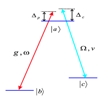
Figure 1: A 3-level $\Lambda$-atom coupled to a classic control and a quantum probe fields with respective detuning $\Delta_{{\rm c}}$ and $\Delta_{{\rm p}}$. When $\Delta_{{\rm p}}$=$\Delta_{{\rm c}}$, the system satisfies the two-photon resonance EIT condition.

In the interaction picture, the interaction part of our Hamiltonian reads ($\hbar=1$)

$$H_{I}=-\Delta_{{\rm p}}S+(g\sqrt{N}aA^{\dagger}+e^{i(\Delta_{{\rm p}}-\Delta_{{\rm c}})t}\Omega T_{+}+h.c.),$$ (1)

in terms of the collective quasi-spin operators

$$S=\sum_{j=1}^{N}\sigma_{{\rm aa}}^{(j)},\ \ A^{\dagger}=\frac{1}{\sqrt{N}}\sum_{j=1}^{N}\sigma_{{\rm ab}}^{(j)},\ \ T_{+}=\sum_{j=1}^{N}\sigma_{{\rm ac}}^{(j)}.$$ (2)

Here $\sigma_{\mu\nu}^{(j)}=|\mu\rangle_{jj}\langle\nu|$ is the flip operator of the $j^{th}$ atom from state $|\mu\rangle_{j}$ to $|\nu\rangle_{j}$ ($\mu,\nu=a,b,c$); and $a^{\dagger}$ ($a$) is the creation (annihilation) operator of the probe light. In the large $N$ limit with low atomic excitations, only a few atoms occupy states $|a\rangle$ or $|c\rangle$ q-defor , and the atomic collective excitations of the atoms behave as bosons since in this case they satisfy the bosonic commutation relation $[A,A^{\dagger}]=1$. When at two-photon resonance defined by $\Delta_{{\rm p}}$=$\Delta_{{\rm c}}$, the Hamiltonian (1) is time-independent and thus there exists the same dark state and dark state polariton as shown before for the one-photon resonant case Sun01 ; 11 .

We note that the above Hamiltonian is expressed in terms of the collective dynamic variables $S$, $A$, $A^{\dagger}$, $T_{-}=(T_{+})^{\dagger}$, and $T_{+}$. To properly describe both the probe light propagation and the cooperative motion of the atomic ensemble stimulated by the two fields, we consider the closed Lie algebra generated by $A$, $A^{\dagger}$, $T_{-}$ and $T_{+}$. To this end a new pair of atomic collective excitation operators

$$C=\frac{1}{\sqrt{N}}\sum_{j=1}^{N}\sigma_{{\rm bc}}^{(j)},\ \ C^{\dagger}=(C)^{\dagger}$$ (3)

are introduced here to form a closed algebra. In the low excitation limit when a few atoms occupy states $|a\rangle$ and $|c\rangle$, the corresponding atomic collective excitations also behave as bosons since they satisfy the bosonic commutation relation $[C,C^{\dagger}]=1$. These atomic collective excitations are independent of each other in the same limit because of the vanishing commutation relations $[A,C]=0,[A,C^{\dagger}]\rightarrow 0$ by a straightforward calculation. Together with the above commutators the following basic commutation relations

$$[S,C^{\dagger}] = 0,[A,S]=A,$$

$$[T_{-},C^{\dagger}] = 0,[T_{+},C^{\dagger}]=A^{\dagger}$$ (4)

define a dynamic symmetry hidden in our dressed atomic ensemble described by the semi-direct-product algebra containing the algebra $SU(2)$ generated by $T_{-}$ and $T_{+}$.

We now calculate the probe field group velocity from the time-dependent Hamiltonian (1). With the help of the above dynamic algebra, we can write down the Heisenberg equations of operators $A$ and $C$ as

$$\dot{A} = -(\Gamma_{{\rm A}}-i\Delta_{{\rm p}})A-ig\sqrt{N}a$$ (5)

$$-ie^{i(\Delta_{{\rm p}}-\Delta_{{\rm c}})t}\Omega C+f_{{\rm A}}(t),$$

$$\dot{C} = -\Gamma_{{\rm C}}C-ie^{-i(\Delta_{{\rm p}}-\Delta_{{\rm c}})t}\Omega A+f_{{\rm C}}(t),$$

where we have phenomenologically introduced the decay rates $\Gamma_{{\rm A}}$ and $\Gamma_{{\rm C}}$ of the states $|a\rangle$ and $|c\rangle$, and $f_{{\rm A}}(t)$ and $f_{{\rm C}}(t)$ are the quantum fluctuation of operators with $\left\langle f_{{\rm\alpha}}(t)f_{{\rm\alpha}}(t^{\prime})\right\rangle\neq 0$, but $\left\langle f_{{\rm\alpha}}(t)\right\rangle=0$, $(\alpha=A,C)$.

To find the steady state solution for the above motion equations of atomic coherent excitation, it is convenient to remove the fast changing factors by making a transformation $C=\tilde{C}e^{-i(\Delta_{{\rm p}}-\Delta_{{\rm c}})t}$. The steady state solution can be achieved from the transformed equations

$$\dot{A} = -(\Gamma_{{\rm A}}-i\Delta_{{\rm p}})A-ig\sqrt{N}a-i\Omega\tilde{C}+f_{{\rm A}}(t),$$

$$\dot{\tilde{C}} = -\Gamma_{{\rm C}}\tilde{C}+i(\Delta_{{\rm p}}-\Delta_{{\rm c}})\tilde{C}-i\Omega A+f_{{\rm C}}(t),$$ (6)

by letting $\dot{A}=\dot{\tilde{C}}=0$. The mean expression of $A$ explicitly obtained is

$$\left\langle A\right\rangle=\frac{-ig\sqrt{N}[\Gamma_{{\rm C}}-i(\Delta_{{\rm p}}-\Delta_{{\rm c}})]\left\langle a\right\rangle}{(\Gamma_{{\rm A}}-i\Delta_{{\rm p}})[\Gamma_{{\rm C}}-i(\Delta_{{\rm p}}-\Delta_{{\rm c}})]+\Omega^{2}}.$$ (7)

It is noticed that the single-mode probe quantum light is described by

$$E(t)=\varepsilon e^{-i\omega t}+h.c.\equiv\sqrt{\frac{\omega}{2V\epsilon_{0}}}ae^{-i\omega t}+h.c.,$$ (8)

where $V$ is the effective mode volume, which for simplicity is chosen to be equal to the interaction volume. While its corresponding polarization is

$$\left\langle P\right\rangle=\left\langle p\right\rangle e^{-i\omega t}+h.c.\equiv\epsilon_{0}\chi\left\langle\varepsilon\right\rangle e^{-i\omega t}+h.c.,$$ (9)

where $\chi=\left\langle p\right\rangle/(\left\langle\varepsilon\right\rangle\epsilon_{0})$ is the susceptibility. Let $\mu$ denote the dipole moment between states $\left|a\right\rangle$ and $\left|b\right\rangle$. The average polarization

$$\left\langle p\right\rangle=\mu\left\langle\sum_{j=1}^{N}\sigma_{{\rm ba}}^{(j)}\right\rangle/V=\frac{\mu\sqrt{N}}{V}\left\langle A\right\rangle$$ (10)

can be expressed here in terms of the average of the exciton operators $A$. Since the coupling coefficient $g=-\mu\sqrt{\frac{\omega}{2V\epsilon_{0}}}$, the susceptibility can be obtained as

$$\chi=\frac{2ig^{2}N(\Gamma_{{\rm C}}-i(\Delta_{{\rm p}}-\Delta_{{\rm c}}))}{\omega[(\Gamma_{{\rm A}}-i\Delta_{{\rm p}})(\Gamma_{{\rm C}}-i(\Delta_{{\rm p}}-\Delta_{{\rm c}}))+\Omega^{2}]}.$$ (11)

The real and imaginary parts $\chi_{1}$ and $\chi_{2}$ of this complex susceptibility $\chi=\chi_{1}+i\chi_{2}$ can be explicitly expressed as

$$\chi_{1} = \frac{[(\Delta_{{\rm p}}-\Delta_{{\rm c}})\Theta-\Gamma_{{\rm C}}\Xi]F}{\Theta^{2}+\Xi^{2}},$$ (12)

$$\chi_{2} = \frac{[\Gamma_{{\rm C}}\Theta+(\Delta_{{\rm p}}-\Delta_{{\rm c}})\Xi]F}{\Theta^{2}+\Xi^{2}},$$ (13)

where $F=2g^{2}N/\omega$ and

$$\Theta = \Gamma_{{\rm A}}\Gamma_{{\rm C}}-\Delta_{{\rm p}}(\Delta_{{\rm p}}-\Delta_{{\rm c}})+\Omega^{2},$$

$$\Xi = \Delta_{{\rm p}}\Gamma_{{\rm A}}+\Gamma_{{\rm A}}(\Delta_{{\rm p}}-\Delta_{{\rm c}}).$$ (14)

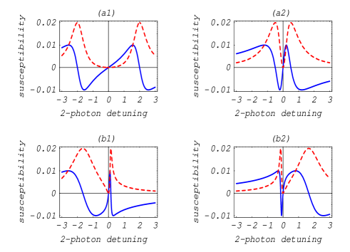
Figure 2: Real part $\chi_{1}$ (solid) and imaginary part $\chi_{2}$ (dashed) of the linear susceptibility vs two-photon detuning $\Delta$ (=$\Delta_{{\rm p}}-\Delta_{{\rm c}}$) in normalized units according to: (a1) $\Omega=2$, $\Delta_{{\rm c}}=0$; (a2) $\Omega=1/2$, $\Delta_{{\rm c}}=0$; (b1,b2) $\Omega=1/2$, $\Delta_{{\rm c}}=\pm 1.5$. Other parameters are given as: $\Gamma_{{\rm A}}=1$, $\Gamma_{{\rm C}}=10^{-4}$, $g\sqrt{N}=100$ and $\omega_{{\rm ab}}=10^{6}$.

It is well-known that $\chi_{1}$ and $\chi_{2}$ are related to dispersion and absorption, respectively. In Fig. 2, $\chi_{1}$ and $\chi_{2}$ are plotted versus the two-photon detuning $\Delta(=\Delta_{{\rm p}}-\Delta_{{\rm c}})$. In Figs. 2(a2,b1,b2), $\Delta_{c}=0,\pm 1.5$ respectively and other parameters are fixed. When $\Delta\rightarrow 0$, both $\chi_{1}$ and $\chi_{2}$ are almost equal to zero. This result is consistent with that in the case of one-photon on-resonance EIT Scullybook ; Lukin01 . This fact shows that the medium indeed becomes transparent when driven by the classical control field as long as the system is prepared in the two-photon resonance ($\Delta=\Delta_{{\rm p}}-\Delta_{{\rm c}}=0$). We also notice that the width of the transparency window (which is determined by $\chi_{2}$) also depends on the Rabi frequency $\Omega$. It can be obviously observed from Fig. 2(a1) (where $\Delta_{{\rm c}}=0$, $\Omega=2$) compared with Fig. 2(a2) (where $\Delta_{{\rm c}}=0$, $\Omega=1/2$).

Next we consider the properties of refraction and absorption of the single-mode probe light in the atomic ensemble medium in more detail. To this end we analyze the complex refractive index

$$n(\omega)=\sqrt{\epsilon(\omega)}=\sqrt{1+\chi},$$ (15)

and generally the real and imaginary parts, $n_{1}$ and $n_{2}$, of $n$ are respectively

$$n_{1} = \sqrt{\frac{[(1+\chi_{1})^{2}+\chi_{2}^{2}]^{1/2}+(1+\chi_{1})}{2}},$$ (16)

$$n_{2} = \sqrt{\frac{[(1+\chi_{1})^{2}+\chi_{2}^{2}]^{1/2}-(1+\chi_{1})}{2}}{\rm sgn}(\chi_{2}),$$ (17)

where ${\rm sgn}(\chi_{2})$=$+1$ $(-1)$ if $\chi_{2}>0$ $(<0)$, $n_{1}$ represents the refractive index of the medium and $n_{2}$ is the associated absorption coefficient. Together with the formulae for the group velocity of the probe light

$$v_{{\rm g}}(\Delta_{{\rm p}},\Delta_{{\rm c}})=\frac{c}{{\it{Re}[n+\omega{\rm d}n/{\rm d}\omega]}}=\frac{c}{n_{1}+\omega\frac{{\rm d}n_{1}}{{\rm d}\omega}}$$ (18)

(where $c$ is the light velocity in vacuum) depending on the frequency dispersion, one can obtain the explicit expression for the group velocity $v_{{\rm g}}$ from Eqs. (12-16) for arbitrary reasonable values of $\Delta_{{\rm p}}$ and $\Delta_{{\rm c}}$. Now, we consider the group velocity of the probe light $v_{{\rm g}}$ for the two-photon resonance, where $\chi_{1}$ and $\chi_{2}$ are almost zero. We find approximately

$$n_{1}\simeq 1+\chi_{1}/2\rightarrow 1,\ \ n_{2}\simeq\chi_{2}\rightarrow 0,$$

and $v_{{\rm g}}$ is given briefly Dogariu as:

$$v_{{\rm g}}(\Delta_{{\rm c}}) = \frac{c}{n_{1}+\omega\frac{{\rm d}n_{1}}{{\rm d}\omega}|_{\Delta_{{\rm p}}=\Delta_{{\rm c}}}}$$ (19)

$$= \frac{c}{1+\frac{\omega}{2}\frac{{\rm d}\chi_{1}}{{\rm d}\omega}|_{\Delta_{{\rm p}}=\Delta_{{\rm c}}}}.$$

It is worth pointing out that, in the calculation of the term $\frac{{\rm d}\chi_{1}}{{\rm d}\omega}$, $\Delta_{{\rm p}}$ $(=\omega-\omega_{{\rm ab}})$ is a function of $\omega$. In what follows we should make a numerical calculation of $v_{{\rm g}}(\Delta_{{\rm c}})$ by means of Eqs. (12,19) (also or Eqs. (12-18)) since its analytical expression is too redundant. According to Eq. (12), the group velocity $v_{{\rm g}}(\Delta_{{\rm c}})$ of the weak probe field depends on $\Delta_{{\rm c}}$, $\Omega$ and $g^{2}N$ when given the other relevant parameters (typically, $\Gamma_{{\rm A}}=1$, $\Gamma_{{\rm C}}=10^{-4}$, $\omega_{{\rm ab}}=10^{6}$).

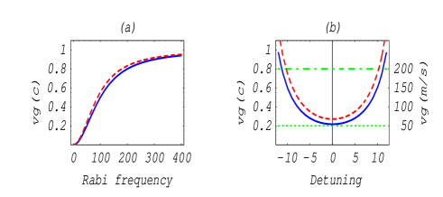
Figure 3: The probe light group velocity $v_{{\rm g}}$ vs: (a) Rabi frequency $\Omega$ [in normalized units] for $\Delta_{{\rm c}}=5$, and $g\sqrt{N}=100$ (blue solid) or $g\sqrt{N}=80$ (red dashed); (b) the detuning $\Delta_{{\rm c}}$ [in normalized units] for $\Omega=2g\sqrt{N}=200$ (green dotted-dashed), or $\Omega=g\sqrt{N}/2=50$ (green dotted), or $\Omega=0.04$ and $g\sqrt{N}=100$ (blue solid), or $\Omega=0.04\Gamma_{{\rm A}}$ and $g\sqrt{N}=80$ (red dashed), where the green dotted-dashed and dotted lines are related to the left axis, and the blue solid and red dashed lines the right axis. Other parameters are given as: $\Gamma_{{\rm A}}=1$, $\Gamma_{{\rm C}}=10^{-4}$ and $\omega_{{\rm ab}}=10^{6}$.

Fig. 3(a) shows the dependence of $v_{{\rm g}}(\Delta_{{\rm c}})$ on the Rabi frequency $\Omega$, where the blue solid (red dashed) line is drawn for $g\sqrt{N}=100$ ($g\sqrt{N}=80$). This provides one with a technique that can be used to accomplish the storage and retrieve of the probe pulse. Initially when the probe field enters into the atomic medium, the Rabi frequency $\Omega$ is very large (relative to g$\sqrt{N}$) and $v_{{\rm g}}\rightarrow c$. When one reduces $\Omega$ adiabatically to zero, $v_{{\rm g}}$ reduces to zero accordingly and then one can store the pulse in the medium. Conversely, if one wants to retrieve the probe pulse, she only needs to increase $\Omega$ adiabatically so as to increase $v_{{\rm g}}$. Fig. 3(b) shows the dependence of $v_{{\rm g}}(\Delta_{{\rm c}})$ vs the common detuning $\Delta_{{\rm p}}$(=$\Delta_{{\rm c}}$) under two-photon resonance EIT. When $\Omega\sim g\sqrt{N}$, $v_{{\rm g}}$ hardly depends on the detuning $\Delta_{{\rm c}}$ and is close to the simplified result $\frac{c}{1+g^{2}N/\Omega^{2}}$ given in Ref. Lukin01 . However, when $\Omega\ll g\sqrt{N}$ as denoted by the blue solid and red dashed curves in Fig. 3(b), $v_{{\rm g}}$ becomes very small and depends on $\Delta_{{\rm c}}$. In the symmetric spectral configuration we find that the group velocity $v_{{\rm g}}$ of the quantum probe light takes its minimum near the zero detuning and $v_{{\rm g}}$ increases when $\mid$$\Delta_{{\rm p}}$$\mid$ increases in the case of two-photon resonance. This theoretical result is consistent with the experimental phenomena as discovered in Ref. Welch2003 when no buffer gases are used.

Finally we notice that, in our model, the density of the medium is proportional to the atom number $N$. Fig. 3(a,b) demonstrates how $v_{g}$ depends on atomic density. In Fig. 3(a) and Fig. 3(b), the blue solid curve is plotted for a denser medium ($g\sqrt{N}=100$ and $g$ is given as constant) than that of the red dashed curve ($g\sqrt{N}=80$). We also find that a denser medium leads to a slower $v_{{\rm g}}$, consistent with our physical intuition.

In the present parameters given in this paper, the group velocity $v_{g}$ is within the zone (0,c). It’s remarked that $v_{g}$ can be negative or superluminal in other $\Lambda$-atoms system as in Ref. Godone ; Dogariu . Different from our EIT system, a system consisted of $\Lambda$-atoms coupled to three optical fields is studied in Godone , and it is the issue of coherent-population-trapping (not EIT) that is considered in Ref. Dogariu . It’s also remarked that a theoretical work Kocharovskaya about the $\Lambda$-atoms EIT system, shows a negative group velocity can appear since the effect of atomic spatial motion (or also the buffer gases) in the hot atoms is considered. Contrarily, the group velocity is always within $(0,c)$ in our EIT system. In our opinion, this difference is mainly due to our ignoring the effect of the atomic spatial motion and the buffer gases in this work.

In conclusion, based on the novel algebraic dynamics method, our theoretical studies on the light propagation in an atomic ensemble with two-photon resonance EIT show a similar phenomenon as discovered in the experiment Welch2003 . Our analysis ignores the generated Stokes field, which is also detected in the above experiment and described in Ref. Stokes01 ; Stokes02 . We also neglect the influence of atomic spatial motion, atomic collisions, and the effects of buffer gases, since in principle these effects can be taken into account as the perturbations in our present study when the atomic ensemble is prepared under enough low temperature.

We acknowledge the support of the CNSF (grant No.90203018), the Knowledge Innovation Program (KIP) of the Chinese Academy of Sciences, and the National Fundamental Research Program of China (No.001GB309310).

References

- (1) S. E. Harris, Phys. Today 50(7), 36 (1997).
- (2) S. Brandt et al., Phys. Rev. A 56, 1063(R) (1997).
- (3) J. Vanier, A. Godone, and F. Levi, Phys. Rev. A 58, 2345 (1998).
- (4) M. D. Lukin et al., Phys. Rev. lett. 79, 2959 (1997).
- (5) L. V. Hau et al., Nature 397, 594 (1999).
- (6) M. M. Kash et al., Phys. Rev. Lett. 82, 5229 (1999).
- (7) C. Liu, Z. Dutton, C. H. Behroozi, and L. V. Hau, Nature 409, 490 (2001).
- (8) D. F. Phillips et al., Phys. Rev. Lett. 86, 783 (2001).
- (9) C. P. Sun, Y. Li, and X. F. Liu, Phys. Rev. Lett. 91, 147903 (2003).
- (10) H. Schmidt and A. Imamoglu, Opt. Lett. 21, 1936 (1996).
- (11) M. O. Scully, M. S. Zubairy, Quantum Optics (Cambridge Univ. Press, Cambridge, 1997)
- (12) M. D. Lukin, S. F. Yelin, and M. Fleischhauer, Phys. Rev. Lett. 84, 4232 (2000).
- (13) M. Fleischhauer and M. D. Lukin, Phys. Rev. Lett. 84, 5094 (2000).
- (14) M. Fleischhauer and M. D. Lukin, Phys. Rev. A 65, 022314 (2002).
- (15) C. Mewes and M. Fleischhauer, Phys. Rev. A 66, 033820 (2002).
- (16) A. V. Turukhin et al., Phys. Rev. Lett. 88, 023602 (2002).
- (17) M. D. Lukin, Rev. Mod. Phys. 75, 457 (2003).
- (18) L. Deng, E. W. Hagley, M. Kozuma, and M. G. Payne, Phys. Rev. A 65, 051805(R) (2002).
- (19) M. Kozuma et al., Phys. Rev. A 66, 031801(R) (2002).
- (20) A. D. Greentree et al., Phys. Rev. A 65, 053802 (2002).
- (21) O. Kocharovskaya, Y. Rostovtsev, and M. O. Scully, Phys. Rev. Lett. 86, 628 (2001).
- (22) E. E. Mikhailov, Y. V. Rostovtsev, and G. R. Welch, quant-ph/0309173.
- (23) Y. X. Liu, C. P. Sun, S. X. Yu, and D. L. Zhou, Phys. Rev. A 63, 023802 (2001).
- (24) A. Godone, F. Levi, and S. Micalizio, Phys. Rev. A 65, 033802 (2002).
- (25) A. Dogariu, A. Kuzmich, and L. J. Wang, Phys. Rev. A 63, 053806 (2001).
- (26) M. D. Lukin, M. Fleischhauer, A. S. Zibrov, H. G. Robinson, V. L. Velichansky, L. Hollberg, and M. O. Scully, Phys. Rev. Lett. 79, 2959 (1997).
- (27) M. M. Kash et al., Phys. Rev. Lett. 82, 5229 (1999).