Analysis and interpretation of high transverse entanglement in optical parametric down conversion

Abstract

Quantum entanglement associated with transverse wave vectors of down conversion photons is investigated based on the Schmidt decomposition method. We show that transverse entanglement involves two variables: orbital angular momentum and transverse frequency. We show that in the monochromatic limit high values of entanglement are closely controlled by a single parameter resulting from the competition between (transverse) momentum conservation and longitudinal phase matching. We examine the features of the Schmidt eigenmodes, and indicate how entanglement can be enhanced by suitable mode selection methods.

Nonclassical correlation among photons has been one of the central topics in quantum optics and quantum communication. In particular, the property of quantum entanglement is now recognized as the key to accomplishments exceeding the limit imposed by classical physical laws. Entangled photons are experimentally available through optical spontaneous parametric downconversion (PDC). Such highly correlated photons have been employed in fundamental experiments, e.g., to test the violation of Bell’s inequality bell1 , and to demonstrate quantum teleportation tele1 . Significantly, down conversion photons provide quantum entanglement in a rich diversity of forms beyond polarization Bell states. For example, one has continuous entanglement in field frequencies huang ; Ian , energy-time variables energy1 and momenta momentum . Altogether, counting the discrete polarization and orbital angular momentum variables angular1 ; angular2 ; angular3 , a full quantum characterization of just two-photon states already requires multiple parameters and the term ‘hyper-entanglement’ has been proposed in order to emphasize the complex structure of such quantum states multi1 .

Here we focus on PDC entanglement that is associated with the transverse wavevectors of signal and idler photon pairs. We are especially interested in ways to reach states of anomalously high entanglement. The PDC quantum state is sometimes called a biphoton Klyshko . Biphoton correlation is experimentally accessible and several investigations have addressed this topic in regard to the underlying orbital angular momentum structure angular1 ; angular2 ; Torres and applications in quantum imaging imaging1 are being explored, including comparison with two-beam correlation using spatially coherent classical light boyd-etal . In this note we approach the subject using the single-sum Schmidt decomposition technique knight , which yields for the first time a complete characterization of the existing entanglement by determining the natural set of bi-orthogonal mode pairs. This is in contrast to studies based on familiar double-sum expansions in Gauss-Laguerre or Gauss-Hermite modes.

To begin with, we consider the signal and idler photons of PDC under the so-called type-II phase matching condition. The two photons are distinguished by their orthogonal polarizations. The explicit forms of biphoton states in three dimensional space are complicated by the details of crystal properties and pump pulse profiles rubin . However, under plausible assumptions in the paraxial approximation, the dependence of longitudinal components of the wavevectors $k_{z}$ and $q_{z}$ may be eliminated in the monochromatic limit angular2 ; monken . Denoting ${\bf k}_{\bot}$ and ${\bf q}_{\bot}$ as transverse wavevectors of the signal and idler photons, the biphoton state takes the approximate form: $\left|\Psi\right\rangle=\int d{\bf k}_{\bot}\int d{\bf q}_{\bot}~{}C\left({{\bf k}_{\bot},{\bf q}_{\bot}}\right)\left|{{\bf k}}_{\bot},{{\bf q}_{\bot}}\right\rangle.$ Here the biphoton amplitude is given by angular2 ; monken ,

$$C\left({{\bf k}_{\bot},{\bf q}_{\bot}}\right)={\cal E}_{p}({{\bf k}_{\bot}+{\bf q}_{\bot}})\Delta({{\bf k}_{\bot}-{\bf q}_{\bot}}),$$ (1)

where ${\cal E}_{p}({\bf k}_{\bot}+{\bf q}_{\bot})$ describes the transverse profile of the pump field in wavevector space, and $\Delta({\bf k}_{\bot}-{\bf q}_{\bot})$ is a purely geometrical function that will be specified later. Note that if the amplitude $C({\bf k}_{\bot},{\bf q}_{\bot})$ were to separate into factors depending only on ${\bf k}_{\bot}$ and ${\bf q}_{\bot}$, then the state $|\Psi\rangle$ would be factorable (not entangled).

The Schmidt decomposition of $C({\bf k}_{\bot},{\bf q}_{\bot})$ corresponds to the expansion,

$$C\left({{\bf k}_{\bot},{\bf q}_{\bot}}\right)=\sum\limits_{n=0}^{\infty}{\sqrt{\lambda_{n}}}u_{n}({\bf k}_{\bot})v_{n}({\bf q}_{\bot})$$ (2)

where $u_{n}({\bf k}_{\bot})$ and $v_{n}({\bf q}_{\bot})$ are Schmidt modes defined by eigenvectors of the reduced density matrices for the signal and idler photons respectively, and $\lambda_{n}$ are the corresponding eigenvalues knight . Thus the mode functions $u_{n}$ form a complete and orthonormal set, and the same is true for the $v_{n}$. Because density matrices always have finite trace, the Schmidt decomposition is always discrete, even when the original specification of the state is naturally continuous, or doubly continuous as in the present situation. This discreteness is intrinsic, independent of any artificial box boundary conditions.

The Schmidt decomposition (2) provides the information eigenstates of the two-particle system, which characterizes the structure of entanglement by providing two important pieces of information not available otherwise. First, the Schmidt single-sum form of decomposition reveals exactly how the photons are paired, i.e., if a signal photon is detected in the mode $u_{n}$, then with certainty the idler photon must be in the mode $v_{n}$. Second, the Schmidt eigenvalues $\lambda_{n}$ serve to measure the degree of entanglement. This is usually discussed in terms of the entanglement entropy $E=-\sum\nolimits_{n}{\lambda_{n}}\log_{2}\lambda_{n}$. However, a more transparent and experimentally more direct measure of entanglement is the ‘average’ number of Schmidt modes involved. The Schmidt number (or participation ratio) $K$ provides this average: $K\equiv 1/\sum\nolimits_{n}{\lambda_{n}^{2}}$. The larger the value of $K$, the higher the entanglement BellK . We remark that the maximum value of $K$ is governed by the volume of accessible phase space of the system under relevant physical constraints such as energy-momentum conservation.

We first examine a class of biphoton amplitudes in which both ${\cal E}_{p}$ and $\Delta$ are represented by gaussian functions:

$$C_{g}({\bf k}_{\bot},{\bf q}_{\bot})={\cal N}_{g}e^{{-|{\bf k}_{\bot}+{\bf q}_{\bot}|^{2}/\sigma_{\bot}^{2}}}e^{-b^{2}|{\bf k}_{\bot}-{\bf q}_{\bot}|^{2}}.$$ (3)

Here ${\cal N}_{g}$ is a normalization constant, and the parameters $\sigma_{\bot}$ and $b^{-1}$ are the widths of the respective gaussians, to which we give physical meaning below. With this amplitude, it can be shown that the Schmidt eigenmodes are simply the energy eigenfunctions of a two-dimensional isotropic harmonic oscillator. The probability of finding a mode (in polar coordinates) with radial and angular quantum numbers $n$ and $m$ is proportional to $\xi^{2n+|m|}$, where $\xi=({1-{b\sigma_{\bot}}})^{2}/\left({1+b\sigma_{\bot}}\right)^{2}$. This leads to a very convenient closed form for the Schmidt number:

$$K=\frac{1}{4}\Big{(}b\sigma_{\bot}+\frac{1}{b\sigma_{\bot}}\Big{)}^{2}.$$ (4)

Thus, $K$ increases as the “control parameter” $b\sigma_{\bot}$ increases or decreases, i.e., for both $b\sigma_{\bot}\gg 1$ and $b\sigma_{\bot}\ll 1$ (see Fig. 1). It is interesting that $K$ can be expressed in terms of the variance of the transverse wavevector components, $K^{1/2}=\left\langle{q_{j}^{2}}\right\rangle/\sqrt{\left\langle{s_{+j}^{2}}\right\rangle\left\langle{s_{-j}^{2}}\right\rangle}$, where $s_{\pm j}=(k_{j}\pm q_{j})/\sqrt{2}$ with the subscript $j$ referring to a component on the transverse $xy$ plane. Such an expression connects the abstract measure of entanglement with observable fluctuations.

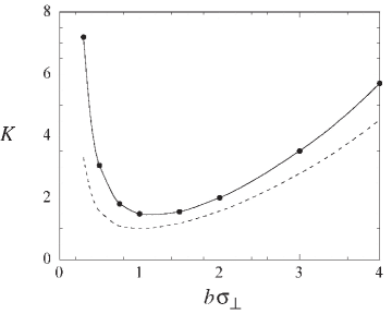
Figure 1: Participation ratio $K$ as a function of $b\sigma_{\bot}$ for the biphoton amplitude $C_{g}$ (dash line) and $C_{s}$ (solid line).

The biphoton amplitude $C_{g}$ can be recognized as a continuous representation of two-mode squeezed states, and these states maximize the EPR correlation for a given amount of entanglement cirac . Eq. (4) provides a useful estimation of degree of entanglement according to the widths of the functions ${\cal E}_{p}({\bf k}_{\bot}+{\bf q}_{\bot})$ and ${\Delta}({\bf k}_{\bot}-{\bf q}_{\bot})$. In practice, $\Delta$ is determined by phase matching in the longitudinal direction, and it is generally not a gaussian. We now follow Monken, et al. monken and consider another class of biphoton amplitude:

$$C_{s}({\bf k}_{\bot},{\bf q}_{\bot})={\cal N}_{s}e^{{-|{\bf k}_{\bot}+{\bf q}_{\bot}|^{2}/\sigma_{\bot}^{2}}}{\rm sinc}\left[{-b^{2}|{{\bf k}_{\bot}-{\bf q}_{\bot}}|^{2}}\right].$$ (5)

Here the transverse profile of the pump field ${\cal E}_{p}$ is treated as a gaussian, and this gives physical meaning to the width $\sigma_{\bot}$, and ${\cal N}_{s}$ is a normalization constant. We have used the subscript $s$ in order to emphasize that $\Delta({{\bf k}_{\bot}-{\bf q}_{\bot}})$ is now taken as the sinc function arising from longitudinal momentum mismatch in the PDC crystal. Spatial coherence is the physical effect that determines $b$ via the relation $b^{2}=cL/4\omega_{p}$, where $L$ is the length of the crystal and $\omega_{p}$ is the pump frequency.

The amplitude (5) is an approximation to actual biphoton states realized in laboratories. This is because technical details involving dispersion and birefringence effects are omitted. However, it captures the main features imposed by conservation of energy and momentum, which are the key constraints on the state in the two-photon Hilbert space. To more fully appreciate (5) in terms of conservation rules, one can see first that the gaussian with the argument ${\bf k}_{\bot}+{\bf q}_{\bot}$ is merely a statement of the uncertainty in transverse momentum conservation, and second that the sinc function’s argument expresses energy conservation $\omega_{s}=\omega_{i}=\omega_{p}/2$ in practice monken .

In several previous studies of biphoton states, the sinc function was approximated by unity in the small $L$ limit (or equivalently the Fourier transform of $\Delta$ was approximated by a delta function) angular2 ; Torres . However, such an approximation is inapplicable to our Schmidt analysis here because the corresponding $C_{s}({\bf k}_{\bot},{\bf q}_{\bot})$ would be unbounded on the ${\bf k}_{\bot}=-{\bf q}_{\bot}$ manifold. Since the sinc function ultimately limits the accessible transverse wave vectors, it has to be fully accounted for in the equation. We also note that exact analogs of the sum and difference arguments in (5) appear in wave functions of entangled states of two massive particles when expressed in terms of center of mass and relative coordinates Fedorov-etal .

To carry out the complete Schmidt decomposition of (5), we make use of polar coordinates, writing: ${\bf k}_{\bot}=(k_{\bot}\cos\theta_{k},~{}k_{\bot}\sin\theta_{k})$ and ${\bf q}_{\bot}=(q_{\bot}\cos\theta_{q},~{}q_{\bot}\sin\theta_{q})$. The biphoton amplitude can be decomposed in the form: $C_{s}({\bf k}_{\bot},{\bf q}_{\bot})=\sum\nolimits_{m}{{{e^{im(\theta_{k}-\theta_{q})}}}}\sqrt{P_{m}}F_{m}(k_{\bot},q_{\bot})/2\pi,$ where $F_{m}(k_{\bot},q_{\bot})$ is a function of magnitude $k_{\bot}$ and $q_{\bot}$, and is normalized according to $\int_{0}^{\infty}{\int_{0}^{\infty}{}|F_{m}(k_{\bot},q_{\bot})|^{2}k_{\bot}q_{\bot}}dk_{\bot}dq_{\bot}=1$. We identify the integer $m$ as a quantum number of orbital angular momentum. Therefore $P_{m}$ is the probability of finding the two photons with opposite orbital angular momentum numbers $m$ and $-m$.

Further decomposition of $F_{m}(k_{\bot},q_{\bot})\sqrt{k_{\bot}q_{\bot}}$ is a simpler task due to its lower dimensionality as compared with $C_{s}({\bf k}_{\bot},{\bf q}_{\bot})$. According to the Schmidt decomposition scheme, we have: $F_{m}(k_{\bot},q_{\bot})\sqrt{k_{\bot}q_{\bot}}=\sum\nolimits_{n}{\sqrt{\gamma_{n,m}}}\phi_{n,m}(k_{\bot})\phi_{n,m}(q_{\bot})$, where the $\phi_{n,m}$ are the same for idler and signal photons because of the symmetry assumed in Eq. (5). Consequently the Schmidt decomposition of the biphoton amplitude reads:

$$C_{s}({\bf k}_{\bot},{\bf q}_{\bot})=\sum\limits_{m=-\infty}^{\infty}\sum\limits_{n=0}^{\infty}\sqrt{\lambda_{nm}}u_{n,m}({\bf k}_{\bot})u_{n,-m}({\bf q}_{\bot})$$ (6)

where $\lambda_{nm}\equiv P_{m}\gamma_{nm}$ and $u_{n,m}({\bf k}_{\bot})\equiv e^{im\theta_{k}}\phi_{n,m}(k_{\bot})/\sqrt{2\pi k_{\bot}}$ are normalized Schmidt mode functions in wavevector space. Eq. (6) reveals that quantum entanglement involves orbital angular momenta and the magnitude of transverse wavevectors.

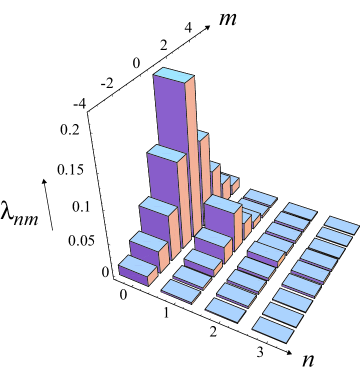
Figure 2: Distribution of $\lambda_{nm}$ of the biphoton amplitude $C_{s}$ with $b\sigma_{\bot}=0.25$.

The gaussian and the sinc function in (5) compete with each other by enforcing correlations in opposite directions. High entanglement is achieved only when one of them becomes dominant, i.e., $\sigma_{\bot}b\gg 1$ or $\sigma_{\bot}b\ll 1$. We have numerically performed the Schmidt decomposition for various values of $\sigma_{\bot}b$. In Fig. 1, we show the Schmidt number $K=1/\sum\nolimits_{nm}\lambda_{nm}^{2}$ as a function $\sigma_{\bot}b$. Consistent with the description above, we see that either a decrease or increase in $\sigma_{\bot}b$ can lead to an increased degree of entanglement. For example, $K\approx 7.2$ when $\sigma_{\bot}b=0.3$. The minimum Schmidt number $K\approx 1.4$ occurs at $\sigma_{\bot}b\approx 1$. The figure also indicates that $C_{s}$ is more entangled than $C_{g}$ at the same parameter value $\sigma_{\bot}b$.

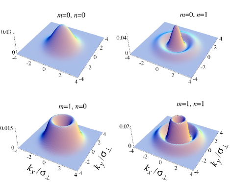
Figure 3: An illustration of first few Schmidt eigenmodes $|u_{n,m}({\bf k}_{\bot})|^{2}$ of the biphoton amplitude $C_{s}$ with $b\sigma_{\bot}=0.25$.

To learn how various modes contribute to the entanglement, we plot in Fig. 2 the distribution of $\lambda_{nm}^{2}$ for the case $b\sigma_{\bot}=0.25$. Such a control parameter value corresponds to a moderately high entanglement regime where conservation of transverse momentum dominates. Small values of $b\sigma_{\bot}$ are typically accessible in experiments using very thin crystals. In Fig. 2 we clearly see that most probabilities are found on the $n=0$ manifold, where the quantum number $n$ equals the number of nodes in the radial direction (Fig. 3). Therefore quantum entanglement is mainly manifest in the angular correlations. In fact, the nature of quantum entanglement can be appreciated from the probability distribution associated with the photon amplitude (Fig. 4). Along the $k=q$ manifold, we see a narrow peak emerge near $\Delta\theta=\theta_{k}-\theta_{q}=\pi$. For smaller values of $b\sigma_{\bot}$ (i.e., higher entanglement), the more pronounced is the peak observed. In other words ${\bf k}_{\bot}$ is almost locked near $-{\bf q}_{\bot}$ for sufficiently large transverse wavevectors. This demonstrates an interesting connection between quantum entanglement and localization in the transverse momentum space. In fact, recent studies have begun to examine the role of entanglement in localization problems Fedorov-etal ; rau .

Fig. 4 suggests that wave vectors with large transverse magnitude are ‘more entangled’. Therefore higher entanglement may be achieved by simply choosing wavevectors with sufficiently large transverse components. This may be realized by adopting certain filtering procedures. As a demonstration, we consider an amplitude

$${\cal A}({\bf k}_{\bot},{\bf q}_{\bot})=C_{s}({\bf k}_{\bot},{\bf q}_{\bot})\theta(k_{\bot}-\mu_{c})\theta(q_{\bot}-\mu_{c})$$ (7)

in which low transverse wavevectors smaller than $\mu_{c}$ are removed by the unit step functions $\theta(x)$. We have performed a Schmidt decomposition of ${\cal A}({\bf k}_{\bot},{\bf q}_{\bot})$ numerically. For the case $b\sigma_{\bot}=0.25$ and $\mu_{c}=2\sigma_{\bot}$, the corresponding Schmidt number is found to be $K\approx 17.2$. This is substantially higher than the original value $K=10.2$. The enhancement is more drastic for the almost disentangled case $b\sigma_{\bot}=1$. In this case we find $K\approx 26$ by using $\mu_{c}=\sigma_{\bot}$. Such an enhancement via amplitude filtering exploits the long tail of the sinc function, and it has a cost in terms of detection rate. Physically it means that there is uncertainty of projecting the two photon amplitude onto ${\cal A}({\bf k}_{\bot},{\bf q}_{\bot})$. For the $b\sigma_{\bot}=1$ example above, the probability of finding the system in ${\cal A}({\bf k}_{\bot},{\bf q}_{\bot})$ is about $6\%$.

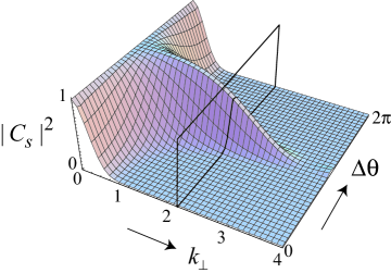
Figure 4: A plot of the two photon amplitude square $|C_{s}({\bf k}_{\bot},{\bf q}_{\bot})|^{2}$ in the $k_{\bot}=q_{\bot}$ subspace. For convenience, the peak value is normalized to one. A cutting plane is shown for the entanglement enhancement scheme discussed in the text. The parameter is $b\sigma_{\bot}=0.25$.

To summarize, we described a method to analyze and interpret physically realistic cases of high transverse entanglement in parametric down conversion, based on the Schmidt decomposition method. For the two classes of two-photon amplitudes defined by $C_{g}$ and $C_{s}$, the degree of entanglement is controlled by a single parameter $b\sigma_{\bot}$. We determined the Schmidt number as a function of $b\sigma_{\bot}$ and identified two experimentally accessible regimes $b\sigma_{\bot}\gg 1$ and $b\sigma_{\bot}\ll 1$ in which values of entanglement higher than reported to date can be studied. In addition we proposed a method to enhance entanglement via large transverse wave vector selection. In fact one sees many possibilities to engineer entanglement through mode selection and manipulation of the shape of the pump pulse profile Torres . The Schmidt decomposition presented here provides a basic framework for investigation of such possibilities.

Acknowledgments: We acknowledge conversations with colleagues, including K. Banaszek, K.W. Chan, M.V. Fedorov, A. Gatti, J. Howell, M. Ivanov, A. Sergienko and I.A. Walmsley, and support from grants NSF PHY00-72359 and ARO DAAD19-99-1-0215, and RGC Project No. 401603.

References

- (1) Z.Y. Ou and L. Mandel, Phys. Rev. Lett. 61, 50 (1988); Y.H. Shih and C.O. Alley, Phys. Rev. Lett. 61, 2921 (1988).
- (2) D. Bouwmeester et al., Nature 390, 575 (1997); D. Boschi et al., Phys. Rev. Lett. 80, 1121 (1998).
- (3) H. Huang and J.H. Eberly, J. Mod. Opt. 40, 915 (1993).
- (4) C.K. Law, I.A. Walmsley, and J.H. Eberly, Phys. Rev. Lett. 84, 5304 (2000); W.P. Grice, A.B. U’Ren, and I.A. Walmsley, Phys. Rev. A 64, 063815 (2001).
- (5) P.G. Kwiat, A. M. Steinberg, and R.Y. Chiao, Phys. Rev. A 47, R2472 (1993); J. Brendel et al., Phys. Rev. Lett. 82, 2594 (1999).
- (6) J.G. Rarity and P.R. Tapster, Phys. Rev. Lett. 64, 2495 (1990).
- (7) A. Mair et al., Nature 412, 313 (2001).
- (8) S. Franke-Arnold et al., Phys. Rev. A 65, 033823 (2002).
- (9) H.H. Arnaut and G.A. Barbosa, Phys. Rev. Lett. 86, 5209 (2001); G.A. Barbosa and H.H. Arnaut, Phys. Rev. A 65, 053801 (2002).
- (10) P.G. Kwiat, J. Mod. Opt. 44, 2173 (1997); M. Atature et al., Phys. Rev. A 65, 023808 (2002).
- (11) D.N. Klyshko, JETP Lett. 6, 23 (1967).
- (12) J.P. Torres et al., Phys. Rev. A 67, 052313 (2003).
- (13) A. Gatti, E. Brambilla, and L.A. Lugiato, Phys. Rev. Lett. 90, 133603 (2003); A.F. Abouraddy et al., Phys. Rev. Lett. 87, 123602 (2001).
- (14) R.S. Bennink, S.J. Bentley, and R.W. Boyd, Phys. Rev. Lett. 89, 113601 (2002).
- (15) See A. Peres, Quantum Theory: Concepts and Methods (Kluwer Academic, 1995), and A. Ekert and P.L. Knight, Am. J. Phys. 63, 415 (1995).
- (16) M.H. Rubin, Phys. Rev. A 54, 5349 (1996).
- (17) C.H. Monken, P.H. Souto Ribeiro, and S. Padua, Phys. Rev. A 57, 3123 (1998); S.P. Walborn, A.N. de Oliveira, and C.H. Monken, Phys. Rev. Lett. 90, 143601 (2003).
- (18) See R. Grobe, K. Rza̧żewski and J.H. Eberly, J. Phys. B 27, L503 (1994). A disentangled (product) state corresponds to , i.e., there is only one term in the Schmidt decomposition. Bell states of two-photon polarization have . Only two-particle states in continuous Hilbert spaces can comprise a large number of Schmidt modes and have very large values.
- (19) G. Giedke et al., Phys. Rev. Lett. 91, 107901 (2003).
- (20) We have recently analyzed entanglement arising in two-particle breakup of massive particles, as in nuclear fission or molecular dissociation. See M.V. Fedorov et al., to be submitted, 2003.
- (21) A connection between entanglement and localization of two particles was recently discussed by A.V. Rau, J.A. Dunningham, and K. Burnett, Science 301, 1081 (2003).