Pulse-driven near-resonant quantum adiabatic dynamics: lifting of quasi-degeneracy

Abstract

We study the quantum dynamics of a two-level system driven by a pulse that starts near-resonant for small amplitudes, yielding nonadiabatic evolution, and induces an adiabatic evolution for larger amplitudes. This problem is analyzed in terms of lifting of degeneracy for rising amplitudes. It is solved exactly for the case of linear and exponential rising. Approximate solutions are given in the case of power law rising. This allows us to determine approximative formulas for the lineshape of resonant excitation by various forms of pulses such as truncated trig-pulses. We also analyze and explain the various superpositions of states that can be obtained by the Half Stark Chirped Rapid Adiabatic Passage (Half-SCRAP) process.

I Introduction

Coherent superposition of states is a key concept of comtemporary quantum physics, for example in quantum communication and computing through entangled states (see e.g. entang ). It is well known that various superpositions of states can be created in a two-level atom (states $\left|-\right\rangle$ and $\left|+\right\rangle$) travelling through a laser (or equivalently for a cold atom driven by a pulsed laser) or through a cavity. If the population initially resides in the ground state $\left|-\right\rangle$, a laser-induced one-photon resonant process leads to a superposition at the end of the interaction [in the rotating wave approximation (RWA)] of the form

$$\left|\psi\right\rangle=\cos\int_{t_{i}}^{t_{f}}\frac{\Omega(t)}{2}dt\ \left|-\right\rangle-ie^{-i\omega t}\sin\int_{t_{i}}^{t_{f}}\frac{\Omega(t)}{2}dt\ \left|+\right\rangle,$$ (1)

where $\Omega(t)$ is the Rabi frequency (assumed real positive) proportional to the pulse envelope and the coupling, that is integrated between $t_{i}$ and $t_{f},$ the initial and final times of interaction, and $\omega$ is the optical frequency. In a one-photon resonant cavity, prepared in a Fock state $\left|n+1\right\rangle$, $n\geq 0$, the counterpart of Eq. (1) reads

$$\left|\psi\right\rangle =\cos\left(\sqrt{n+1}\int_{t_{i}}^{t_{f}}\frac{\Omega(t)}{2}dt\right)\left|-,n+1\right\rangle$$

$$-i\sin\left(\sqrt{n+1}\int_{t_{i}}^{t_{f}}\frac{\Omega(t)}{2}dt\right)\left|+,n\right\rangle,$$ (2)

where $\left|i,k\right\rangle$ represents the atomic bare state $\left|i\right\rangle$ dressed by $k$ photons of the cavity. For instance, a half superposition is achieved when the Rabi frequency area is $\pi/2$. From the practical point of view, this process requires the precise control of the effectively interacting pulse shape, i.e. in the case of a travelling atom, this requires a well-controlled and homogenous velocity and the control of the characteristics of the intersection between laser and atomic beam. As a consequence, this process is said to be non-robust with respect to the pulse amplitude. Creation of coherent superpositions of states by adiabatic passage is of great interest since this process requires a sufficiently large pulse area, but not precisely defined: hence it is robust with respect to fluctuations of the interaction and also to partial knowledge of atomic and field parameters.

The analysis of adiabatic evolution and its leading corrections is well-understood in the case of exact (one-photon) resonance and in the far from resonance case. The behavior in theses two exterme cases is qualitatively different. As a consequence, in the intermediate regime that we will characterize as quasi-resonant, there is a competition of different effects that to our knowledge has not been studied quantitatively. The goal of this article is to present a detailled analysis of this intermediate regime, whose understanding is important for practical applications. We obtain the results combining insights from exactly solvable models with approximations obtained by perturbative techniques in different regimes. We test the quantitative validity of our results by comparison with direct numerical simulations.

We can identify the different known regimes of the dynamics in a two-level system considering a detuning $\Delta$. We denote by $T$ the characteristic time of the rising (and falling) of the pulse. The resonant case is defined as

$$T\Delta\ll 1.$$ (3)

We can reintepret the formulas (1) and (2) and extend them to the case of multiphoton resonant processes with adiabatic pulses as follows Holthaus ; Guerin_PRA97 ; review . In the case of an exact $n-$photon resonance, the two relevant dressed states $\left|-,n\right\rangle$ and $\left|+,0\right\rangle$ can be considered, before the rising of the pulse, as exactly degenerate with respect to the dynamics. The pulse rising induces a lifting of the degeneracy, which leads to a splitting of the dynamics along the two eigenstate branches. It is important to note that this splitting is instantaneous at the beginning of the pulse only in the case of one-photon resonance $n=1$ and in the two-photon case $n=2$ review . Higher multiphoton processes involve Stark shifts which modify the splitting. The $n=1$ case induces an equal splitting along the two eigenstate branches. These two branches are next followed adiabatically by the dynamics if the pulse envelopes are slow enough. One can define dynamical phases which are the areas between the associated dressed eigenenergies. When later the pulse falls, the dynamics faces the symmetrically inverse problem of the creation of degeneracy with a recombination (instantaneous for $n=1$ and $n=2$) leading to the interference of the two branches at the very end of the process. The resulting final transfer depends on (i) the way in which the splitting (and recombination) occurs (in amplitude and phase), and (ii) the difference of the dynamical phases. In the case of a complete transfer, the process has been named generalized or multiphoton $\pi$-pulse. This process is not robust because the splitting (and recombination) and the difference of the dynamical phases depend on the parameters. Moreover, numerics shows that it is much more sensitive to the detuning from the multiphoton resonance than to the pulse shape Just ; Korolkov .

In the opposite regime far from the resonance defined by the condition

$$T\Delta\gg 1,$$ (4)

the dynamics is at all time adiabatic in the sense that it follows the single dressed eigenstate whose eigenvalue is continuously connected to the one associated to the initial bare state. The nonadiabatic corrections (exponentially small for smooth pulses), that produce losses into the other eigenstate have been extensively studied, e.g. in Berman .

If the detuning is additionally time dependent (induced by a direct frequency chirping or by an additional off-resonant pulse which Stark shifts the states) and if the condition (4) is satisfied during the rising and the falling of the pulse, it has been shown Guerin_PR00 ; Yatsenko_PR01 ; review that the topology of the dressed eigenenergy surfaces, as functions of the effective time-dependent external field parameters, allows to determine the various possible population transfers. The main ingredient is a global adiabatic passage along one eigenstate combined with local crossings of resonances which appear as conical intersections and that can be precisely determined from the eigenenergy surfaces. This adiabatic passage results at the end of the process either in a complete population transfer to the excited state or in a complete return to the ground state. This process in the case of an additional Stark laser, leading to a complete population transfer, has been named Stark Chirped Rapid Adiabatic Passage (SCRAP) Yatsenko_PR99 ; Rickes .

In this paper, we study the intermediate quasi-resonant regimes, defined by the condition

$$T\Delta\sim 1.$$ (5)

They lead to a lifting (and creation) of a quasi-degeneracy. We construct formulas characterizing the dynamics at asymptotic times beyond the lifting of quasi-degeneracy, assuming adiabatic evolution along the two branches.

Resonance between two quantum states and the resulting transitions are mainly understood through the asymptotic limit of the Landau-Zener avoided crossing model Landau ; Zener ; Dykhne ; Davis : A complete transition can be achieved by adiabatic passage beyond the avoided crossing, along the state continuously connected to the initial one. We will show that in the case of pulses with amplitude growing linearly in time, the problem of the lifting of quasi-degeneracy can be interpreted as a half Landau-Zener process Vitanov .

We also solve the problem of the lifting of quasi-degeneracy beyond the half Landau-Zener model, for pulses rising as power of time and as smooth exponential ramps.

In the next section, we describe the model with the different couplings. In Section III, we define the adiabatic states in the model and the conditions for adiabatic evolution along one of the adiabatic states. We show the dynamics when the adiabatic conditions are not satisfied at early times. Section IV and V are devoted to the calculation of the dynamics respectively for linear and exponential rising coupling. In section VI and VII, we analyze the dynamics with perturbation theory in the limits of respectively large and small detuning. On the basis of the results of Sections IV, VI and VII, we give an approximative formula in Section VIII for a power law rising of the coupling. In Sections IX and X, we apply the results to obtain the lineshape of pulsed resonant excitation and to the analysis of the Half-SCRAP process. In Section XI, we present some conclusions and open related problems.

II The model

We study a two-level system (states $\left|-\right\rangle$ and $\left|+\right\rangle$) driven by a near-resonant pulsed laser whose state evolution $\phi(\tau)$ is given by the Schrödinger equation

$$i\hbar\frac{\partial\phi}{\partial\tau}(\tau)=T_{0}\mathsf{H}(\tau)\phi(\tau),\quad\phi(\tau)=\left[\begin{array}[]{c}B_{-}(\tau)\\ B_{+}(\tau)\end{array}\right]\in\mathbb{C}^{2},$$ (6)

with $\left|B_{-}(\tau)\right|^{2}+\left|B_{+}(\tau)\right|^{2}=1$, the scaled time $\tau=t/T_{0}$ and the Hamiltonian in the quasi-resonant approximation Allen ; Shore

$$\mathsf{H}(\tau)=\frac{\hbar}{2}\left[\begin{array}[]{cc}-\Delta(\tau)&\Omega(\tau)\\ \Omega(\tau)&\Delta(\tau)\end{array}\right],$$ (7)

where we have considered the basis $\left\{\left|-\right\rangle,\left|+\right\rangle\right\}$.

We consider the Hamiltonian (7) with a constant detuning

$$\Delta(\tau)=\Delta_{0}>0$$ (8)

and the following models of coupling between the initial $\tau_{i}$ and a final time $\tau_{f}$:

(i) power law rising

$$\Omega(\tau)=\left\{\begin{array}[]{c}\Omega_{0}\tau^{n},\;\tau\geqslant\tau_{i}\\ 0,\;\tau<\tau_{i},\end{array}\right.$$ (9)

with $\tau_{i}=0,$ $\tau_{f}\gtrsim 1$, and falling

$$\Omega(\tau)=\left\{\begin{array}[]{c}\Omega_{0}\left(-\tau\right)^{n},\;\tau\leq\tau_{f}\\ 0,\;\tau>\tau_{f},\end{array}\right.$$ (10)

with $\tau_{i}\lesssim-1$, $\tau_{f}=0$, for an integer $n\geq 1$,

(ii) smooth exponential rising

$$\Omega(\tau)=\Omega_{0}e^{\tau}$$ (11)

with $\tau_{i}\rightarrow-\infty,$ $\tau_{f}\gtrsim 0$, and falling

$$\Omega(\tau)=\Omega_{0}e^{-\tau}$$ (12)

with $\tau_{i}\lesssim 0$, $\tau_{f}\rightarrow+\infty,$ and

(iii) smooth Gaussian

$$\Omega(\tau)=\Omega_{0}e^{-\tau^{2}}$$ (13)

with $\tau_{i}\rightarrow-\infty$ and/or $\tau_{f}\rightarrow+\infty$. We assume $\Omega(\tau)\geq 0$.

We moreover consider for the pulse rising the initial conditions at time $\tau_{i}$: $B_{-}(\tau_{i})=1$, $B_{+}(\tau_{i})=0$.

III Adiabatic and nonadiabatic evolution

III.1 Adiabatic transformation

The adiabatic states $\Phi_{\pm}(\tau)$ are defined as the eigenstates of $\mathsf{H}(\tau)$, associated to the eigenvalues $\lambda_{\pm}(\tau)$:

$$\mathsf{H}(\tau)\Phi_{\pm}(\tau)=\lambda_{\pm}(\tau)\Phi_{\pm}(\tau).$$ (14)

Gathering the adiabatic states in the columns of the unitary matrix $\mathsf{R}(\tau)=\left[\Phi_{-}(\tau),\Phi_{+}(\tau)\right]:$

$$\mathsf{R}(\tau)=\left[\begin{array}[]{cc}\cos\theta(\tau)&\sin\theta(\tau)\\ -\sin\theta(\tau)&\cos\theta(\tau)\end{array}\right]$$ (15)

with

$$\tan 2\theta(\tau)=\frac{\Omega(\tau)}{\Delta(\tau)},\quad 0\leq\theta(\tau)<\pi/2,$$ (16)

giving

$$\mathsf{R}^{\dagger}(\tau)T_{0}\mathsf{H}(\tau)\mathsf{R}(\tau)=\left[\begin{array}[]{cc}\lambda_{-}&0\\ 0&\lambda_{+}\end{array}\right],\quad\lambda_{\pm}(\tau)=\pm\frac{\hbar}{2}T_{0}\delta(\tau)$$ (17)

with

$$\delta(\tau)=\sqrt{\Delta^{2}(\tau)+\Omega^{2}(\tau)},$$ (18)

we can rewrite the Schrödinger equation as

$$i\hbar\frac{\partial}{\partial\tau}\phi_{A}(\tau)=\mathsf{H}_{A}(\tau)\phi_{A}(\tau)$$ (19)

with

$$\mathsf{H}_{A}(\tau)=\frac{\hbar}{2}\left[\begin{array}[]{cc}-T_{0}\delta(\tau)&-i\gamma(\tau)\\ i\gamma(\tau)&T_{0}\delta(\tau)\end{array}\right],$$ (20)

the non-adiabatic coupling

$$\gamma(\tau)\equiv 2\frac{d\vartheta(\tau)}{d\tau}=\frac{\dot{\Omega}(\tau)\Delta(\tau)-\Omega(\tau)\dot{\Delta}(\tau)}{\Delta^{2}(\tau)+\Omega^{2}(\tau)},$$ (21)

and

$$\phi_{A}(\tau)\equiv\left[\begin{array}[]{c}A_{-}(\tau)\\ A_{+}(\tau)\end{array}\right]=\mathsf{R}^{\dagger}(\tau)\phi(\tau)=\mathsf{R}^{\dagger}(\tau)\left[\begin{array}[]{c}B_{-}(\tau)\\ B_{+}(\tau)\end{array}\right].$$ (22)

Since $A_{\pm}(\tau)\equiv\left\langle\pm\right|\left.\phi_{A}(\tau)\right\rangle=\left\langle\Phi_{\pm}(\tau)\right|\left.\phi(\tau)\right\rangle$, one can interpret $\left|A_{\pm}(\tau)\right|^{2}$ as the population of the adiabatic states $\left|\Phi_{\pm}(\tau)\right\rangle$. In the adiabatic limit, mathematically defined as $T_{0}\rightarrow\infty$, the non-adiabatic coupling $\gamma$ can be neglected and the dynamics follows the adiabatic states.

Since $\Omega(\tau)$ and $\Delta(\tau)$ are assumed positive, at times $\tau_{0}$ for which the pulse goes to zero, one has

$$\Omega(\tau_{0})\rightarrow 0,$$ (23)

$\theta(\tau_{0})\rightarrow 0$ and $\phi_{A}(\tau_{0})=\phi(\tau_{0})$, hence

$$A_{-}(\tau_{0})=B_{-}(\tau_{0}),\quad A_{+}(\tau_{0})=B_{+}(\tau_{0}).$$ (24)

III.2 Condition of adiabatic evolution

In this section, we consider the rising of the pulse. Since one considers in the following a constant detuning $\Delta(\tau)=\Delta_{0}$, the dynamics is adiabatic if

$$\widetilde{\gamma}(\tau)\equiv\frac{|\gamma(\tau)|}{2T_{0}\lambda(\tau)}\ll 1.$$ (25)

i.e.

$$\frac{1}{2}\frac{\dot{\Omega}(\tau)\Delta_{0}}{\left(\Delta_{0}^{2}+\Omega^{2}(\tau)\right)^{3/2}}\ll T_{0},$$ (26)

where we have defined the nonadiabatic coefficient $\widetilde{\gamma}(\tau)$ (which appears at the first order of the time-dependent perturbation theory). We assume here that the time $t=T_{0}$ is a characteristic time beyond which the evolution of the system is adiabatic, i.e. without population transfer between adiabatic states. Our goal is to find the population transfer during the characteristic time before adiabaticity.

For times $\tau\sim 1$ (i.e. $t\sim T_{0}$), Eq. (26) for a power law coupling (9) reads

$$2T_{0}\left[\Delta_{0}^{2}+\Omega_{0}^{2}\right]^{3/2}\gg n\Omega_{0}\Delta_{0},$$ (27)

which, using $\Omega_{0}\Delta_{0}/(\Delta_{0}^{2}+\Omega_{0}^{2})\sim 1$, can be roughly simplified as

$$2T_{0}\left[\Delta_{0}^{2}+\Omega_{0}^{2}\right]^{1/2}\gg n.$$ (28)

We assume in this paper that this condition (28) is satisfied for power law couplings. For large detunings defined here as $T_{0}\Delta_{0}\gg n$, the evolution is adiabatic around these times $\tau\sim 1$ for any $\Omega_{0}$ (and is actually adiabatic at anytime if one additionally excludes $\Omega_{0}\gg\Delta_{0}$, as shown below). For intermediate detunings defined as $T_{0}\Delta_{0}\sim n$ (and also for small detunings $T_{0}\Delta_{0}\ll n$), the dynamics is adiabatic for $\tau\sim 1$ only when $T_{0}\Omega_{0}\gg n.$

We can calculate for a power law coupling (9) the scaled time $\tau_{M}=t_{M}/T_{0}$ at which the nonadiabatic coefficient $\widetilde{\gamma}(\tau)$ is maximum:

$$\tau_{M}=\left(\frac{n-1}{2n+1}\right)^{1/2n}\left(\frac{\Delta_{0}}{\Omega_{0}}\right)^{1/n},$$ (29)

which gives the estimates

$$\left\{\begin{array}[]{c}\tau_{M}=0,\text{ for }n=1,\\ \tau_{M}\sim\left(\frac{\Delta_{0}}{\Omega_{0}}\right)^{1/n},\text{ for }n\geq 2\end{array}\right.$$ (30)

and

$$\left\{\begin{array}[]{c}\widetilde{\gamma}(\tau_{M}=0)=\frac{1}{2}\frac{\Omega_{0}}{\Delta_{0}}\frac{1}{T_{0}\Delta_{0}},\text{ for }n=1,\\ \widetilde{\gamma}(\tau_{M})\sim\frac{n}{4}\left(\frac{\Omega_{0}}{\Delta_{0}}\right)^{1/n}\frac{1}{T_{0}\Delta_{0}},\text{ for }n\geq 2.\end{array}\right.$$ (31)

For $n=1$, the nonadiabatic coefficient $\widetilde{\gamma}(\tau)$ decreases monotonically from $\widetilde{\gamma}(\tau_{M}=0)=\frac{1}{2}\frac{\Omega_{0}}{\Delta_{0}}\frac{1}{T_{0}\Delta_{0}}$ to zero, with a width of order $\frac{\Delta_{0}}{\Omega_{0}}$. For $n\geq 2$, it is roughly bell-shaped and symmetric around $\tau_{M}$. This quantity (31) allows to characterize the global adiabaticity: if $\widetilde{\gamma}(\tau_{M})\ll 1$, the dynamics is adiabatic at any time. This implies that detunings such that $\Delta_{0}\gg\Omega_{0}$ induce adiabaticity at all times. For $\Delta_{0}\sim\Omega_{0}$, the dynamics is also adiabatic at all times if the detuning is large $T_{0}\Delta_{0}\gg n$. (The case $\Delta_{0}\sim\Omega_{0}$ and $T_{0}\Delta_{0}\sim n$ is not of interest here since it induces a nonadiabatic dynamics for $t\sim T_{0}$.)

Conversely detunings such that $\Delta_{0}\ll\Omega_{0}$ induce a nonadiabatic dynamics around times $\tau_{M}$. This is this last non trivial case, which is of interest here (accompanied with the condition $T_{0}\Omega_{0}\gg n$ to have adiabaticity beyond $\tau\sim 1$). This case can be described in more detail as follows: during early scaled times of order $\left(\frac{\Delta_{0}}{\Omega_{0}}\right)^{1/n}$, the dynamics is approximately adiabatic for the rising coupling (this initial adiabatic regime occurs only for $n>1$), it is followed by a nonadiabatic dynamics around times $\tau_{M}$ which lasts during times also of order $\left(\frac{\Delta_{0}}{\Omega_{0}}\right)^{1/n}$ (true for any $n\geq 1$), and an adiabatic evolution for times beyond (see Fig. 1).

For exponential and Gaussian couplings, we will consider the non-trivial case $\Delta_{0}\ll\Omega_{0}$ with $T_{0}\Omega_{0}\gg 1$, which allows adiabaticity [through Eq. (26)] for times $\tau\sim 1$.

We will show the universality of this regime for the different couplings considered above.

III.3 Population history

The time evolution of the population $\left|A_{+}(\tau)\right|^{2}=\left|\left\langle\Phi_{+}(\tau)\right|\left.\phi(\tau)\right\rangle\right|^{2}$ in the adiabatic state $\left|\Phi_{+}(\tau)\right\rangle$ is shown on the Fig. 1 for power law risings. One can see the regions of the adiabatic and nonadiabatic evolution according to the analysis given below. For $n=1$ the nonadiabatic evolution, characterized by a change of the population which moves into $\left|\Phi_{+}(\tau)\right\rangle$, starts already for short times and is followed by an adiabatic evolution, characterized by a constant population in $\left|\Phi_{+}(\tau)\right\rangle$ and $\left|\Phi_{-}(\tau)\right\rangle$. For $n>1$ there are time intervals of adiabacity for small and large times. For higher $n$ the early time interval of adiabaticity is longer, since the characteristic time of rising is larger. For larger $\Delta_{0}$ the early time interval of adiabaticity is also longer.

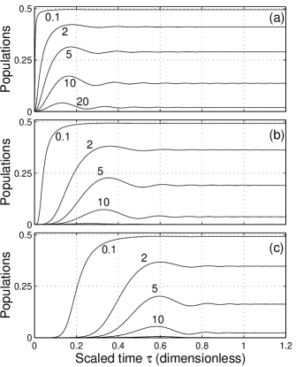
Figure 1: Adiabatic state population history $\left|A_{2}(\tau)\right|^{2}$ for the cases of linear rising coupling $n=1$ (frame a), power law rising with $n=2$ (frame b) and $n=4$ (frame c) for different dimensionless detuning $\Delta_{0}T_{0}$ (indicated close to each curve) and a fixed coupling $\Omega_{0}T_{0}=100$ which allows the condition (28) to be verified for the different cases considered.

IV Lifting and creation of quasi-degeneracy by linearly rising coupling

The problem of lifting of quasi-degeneracy can be solved analytically in the case of linear rising of the coupling [Eq. (9) with $n=1$]. The exact solution of the Schrödinger equation can be found in this case, in terms of the parabolic cylinder functions (see Appendix A). We need to calculate the dynamics at asymptotic times beyond the lifting of quasi-degeneracy when the population of the adiabatic states is time independent.

The initial condition $A_{-}(\tau_{i})=B_{-}(\tau_{i})=1,$ $A_{+}(\tau_{i})=B_{+}(\tau_{i})=0$ leads to the amplitudes of the adiabatic states

$$A_{\pm}(\tau) \rightsquigarrow \frac{1}{\sqrt{2}}\left(a\mp be^{\mp i\varphi}\right)e^{\mp i\left(\chi_{0}+\eta_{d}(\tau)\right)}$$ (32a)

$$\equiv \sqrt{p_{\pm}}\ e^{\mp i\left(\chi_{\pm}+\eta_{d}(\tau)\right)}$$ (32b)

with the transition probabilities

$$p_{\pm} =\frac{1}{2}\left|a\mp be^{i\varphi}\right|=\frac{1}{2}\left(1\mp\sqrt{1-e^{-\pi\omega^{2}}}\cos\varphi\right),$$ (33)

$$\varphi =\arg\Gamma\left(1-i\frac{\omega^{2}}{4}\right)-\arg\Gamma\left(\frac{1}{2}-i\frac{\omega^{2}}{4}\right)+\frac{\pi}{4},$$ (34)

$$\omega =\frac{T_{0}\Delta_{0}}{\sqrt{2T_{0}\Omega_{0}}},$$ (35)

$$a =\frac{1}{\sqrt{2}}\sqrt{1+e^{-\pi\omega^{2}/2}},\ b=\frac{1}{\sqrt{2}}\sqrt{1-e^{-\pi\omega^{2}/2}},$$ (36)

(where $\Gamma$ denotes the Gamma–function) and the phases

$$\chi_{\pm} =\chi_{0}+\arg\left(a\mp be^{i\varphi}\right),$$ (37)

$$\chi_{0} =\arg\Gamma\left(\frac{1}{2}-i\frac{\omega^{2}}{4}\right)-\frac{\omega^{2}}{4}\left(1-\ln\frac{\omega^{2}}{4}\right),$$ (38)

$$\eta_{d}(\tau) =\frac{1}{\hbar}\int_{0}^{\tau}\lambda_{+}(\tau)d\tau=\frac{T_{0}}{2}\int_{0}^{\tau}\sqrt{\Delta_{0}^{2}+\Omega_{0}^{2}\tau^{2}}d\tau.$$ (39)

One can interpret $\sqrt{p_{\pm}}\exp\left(\pm i\chi_{\pm}\right)$ as the probability amplitudes of the adiabatic states from the initial bare state $\left|-\right\rangle$ resulting from the lifting of degeneracy and the splitting of the population. This splitting is accompanied by phases shifts $\pm\chi_{\pm}$. The additional phases $\pm\eta_{d}(\tau)$ given by the time integral of the adiabatic eigenvalues are thus the dynamical phases of the process.

The accuracy of the asymptotics (32) is shown in Fig. 2. At $\tau=1$, we observe already a precision of many digits both in population and phase.

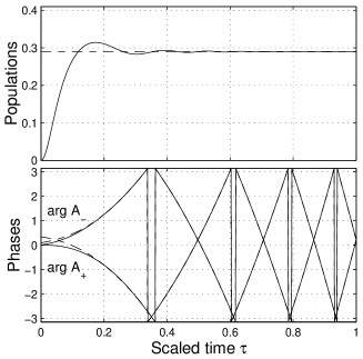
Figure 2: History of adiabatic state population $\left|A_{+}(\tau)\right|^{2}$ [upper frame; numerics: full line, and analytical formula $p_{+}$ (33): dashed line] and phases $\arg A_{\pm}(\tau)$ [lower frame; numerics: full line, and analytical formulae $\mp(\chi_{\pm}+\eta_{d}(\tau))$ given by Eqs. (37) and (39): dashed lines] for the linear rising coupling with $T_{0}\Delta_{0}=5$ and $T_{0}\Omega_{0}=100$ (giving $\omega\approx 0.35$). Phases are plotted in the interval $[-\pi,+\pi[$, which induces artificial jumps that we have connected for a clearer identification.

One essential result is that the adiabatic populations $p_{\pm}$ and the phases $\chi_{\pm}$ depend only on $\omega$ [Eq. (35)]. Their dependence is shown on Fig. 3. The phases $\chi_{+}$ and $\chi_{-}$ go asymptotically to $-\pi/2$ and $0$ respectively. One can remark that $\chi_{-}$ is not very different from zero after (and also during) the lifting of degeneracy for any detuning. This trend has been numerically checked to occur for any $n$.

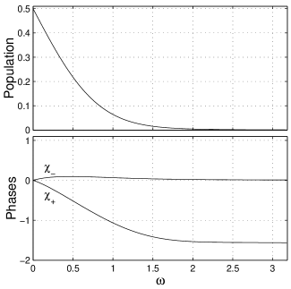
Figure 3: Asymptotic adiabatic state population $\left|A_{+}\right|^{2}$ (33) (upper frame) and phases $\chi_{-}$ and $\chi_{+}$ (37) (lower frame) as functions of the dimensionless quantity $\omega$ for the linear rising of the coupling.

The reversed problem of lifting of quasi-degeneracy, which we called creation of quasi-degeneracy, is induced by a pulse falling to zero [Eq. (9), with $n=1$]. It leads to a recombination of the two adiabatic states. This has been calculated in Appendix A.

V Lifting and creation of quasi-degeneracy by exponentially rising coupling

The problem of lifting and creation of quasi-degeneracy can be also solved analytically in the case of exponentially rising (11) and falling (12) coupling (see Appendix B). The asymptotics of the exact solution can be expressed in terms of the Kummer functions. In the adiabaticity region where the population of the eigenstates is time independent, with the initial condition $A_{-}(\tau_{i})=B_{-}(\tau_{i})=1,$ $A_{+}(\tau_{i})=B_{+}(\tau_{i})=0$ at $\tau_{i}\rightarrow-\infty$, we obtain the amplitudes of the adiabatic states

$$A_{\pm}(\tau)\rightsquigarrow\sqrt{p_{\pm}}\ e^{i\left(\xi\mp\zeta(\tau)\right)}$$ (40)

with the transition probabilities

$$p_{-}=\frac{1}{1+e^{-\pi\varpi}},\quad p_{+}=\frac{e^{-\pi\varpi}}{1+e^{-\pi\varpi}},$$ (41)

the instantaneous dimensionless pulse half-area (which is in fact an instantaneous Rabi frequency half-area)

$$\zeta(\tau)=\frac{T_{0}}{2}\int_{-\infty}^{\tau}\Omega(\tau^{\prime})d\tau^{\prime}=\frac{T_{0}}{2}\Omega_{0}e^{\tau},$$ (42)

the dimensionless detuning

$$\varpi=T_{0}\Delta_{0}$$ (43)

and the phase [given by Eq. (173)]

$$\xi=\arg\Gamma\left(\frac{1}{2}+i\frac{\varpi}{2}\right)+\varpi\ln 2-\frac{\varpi}{2}\ln 2\zeta(\tau_{i}).$$ (44)

(In practice, $\tau_{i}$ is to be taken as a finite large negative number.) The phase $\xi$ of the amplitudes is a common phase for the resulting superposition of adiabatic states. There is no additional relative phase shift during the lifting of degeneracy.

It is remarkable that the transition probabilities depend only on the detuning $\Delta_{0}T_{0}$ (and not on $\Omega_{0}$). Moreover the preceding dynamical phase is here replaced by a pulse area.

The accuracy of the asymptotics (40) is shown in Fig. 4.

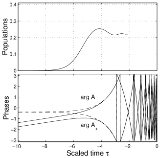
Figure 4: History of adiabatic state population $p_{+}=\left|A_{+}(\tau)\right|^{2}$ [upper frame; numerics: full line, and analytical formula $p_{+}$ (41): dashed line] and phases $\arg A_{\pm}(\tau)$ [lower frame; numerics: full line, and analytical formulae $\xi\mp\zeta(\tau)$ given by Eqs. (44) and (42): dashed lines] for the exponential rising of the coupling with $T_{0}\Delta_{0}=0.4$ and $T_{0}\Omega_{0}=100$.

VI Perturbation theory for large detuning

For large detuning $T_{0}\Delta_{0}$, the evolution of the system is adiabatic at all times (we exclude $\Omega_{0}\gg\Delta_{0}$). We are thus interested here in small nonadiabatic corrections from the initial condition $A_{-}(\tau_{i})=B_{-}(\tau_{i})=1,$ $A_{+}(\tau_{i})=B_{+}(\tau_{i})=0$. It is well known that their main contribution are given by the nonsmoothness of the coupling at the beginning, characterized here by a discontinuous $n^{\text{th}}$ derivative Garrido ; Sancho . In this section we give estimates of corrections beyond.

It is convenient to use the adiabatic basis, in which we use the standard perturbation theory:

$$A_{\pm}(\tau)=A_{\pm}^{\left(0\right)}(\tau)+\varepsilon A_{\pm}^{\left(1\right)}(\tau)+\varepsilon^{2}A_{\pm}^{\left(2\right)}(\tau)+\cdots$$ (45)

with $\varepsilon\equiv 1/\left(T_{0}\left|\Delta_{0}\right|\right)$ and the initial condition $A_{-}^{\left(0\right)}(\tau_{i})=1$, $A_{+}^{\left(0\right)}(\tau_{i})=0$, $A_{\pm}^{\left(n>0\right)}(\tau)=0$. The zeroth order gives

$$A_{-}^{\left(0\right)}(\tau)=e^{i\eta_{d}(\tau)},\qquad A_{+}^{\left(0\right)}(\tau)=0$$ (46)

with the dynamical phase

$$\eta_{d}(\tau)=\frac{1}{\hbar}\int_{0}^{\tau}\lambda_{+}(\tau)d\tau=\frac{T_{0}}{2}\int_{\tau_{i}}^{\tau}\delta(\tau^{\prime})d\tau^{\prime}.$$ (47)

The first order contributions read

$$\varepsilon A_{-}^{\left(1\right)}(\tau) =0$$ (48a)

$$\varepsilon A_{+}^{\left(1\right)}(\tau) =\frac{1}{2}e^{-i\eta_{d}(\tau)}\int_{\tau_{i}}^{\tau}d\tau^{\prime}\gamma(\tau^{\prime})e^{2i\eta_{d}(\tau^{\prime})},$$ (48b)

which give at first order

$$A_{-}(\tau) \approx e^{i\eta_{d}(\tau)}$$ (49a)

$$A_{+}(\tau) \approx\frac{1}{2}e^{-i\eta_{d}(\tau)}\int_{\tau_{i}}^{\tau}d\tau^{\prime}\gamma(\tau^{\prime})e^{2i\eta_{d}(\tau^{\prime})}.$$ (49b)

This shows that the phase of $$A_{-}(\tau) n=1 \chi_{-} P_{+}(\tau)\equiv\left|A_{+}(\tau)\right|^{2} \tau\rightarrow+\infty$$ is approximately given by only the dynamical phase. This is consistent with what we obtained for , where (37) was not very different from zero during the lifting of degeneracy. The transition probability at the first order at large times is given asymptotically by

$$P_{+}(\tau)\rightsquigarrow\frac{1}{4}\left|\int_{\tau_{i}}^{\tau}d\tau\ \gamma(\tau)e^{2i\eta_{d}(\tau)}\right|^{2}.$$ (50)

For consistency of the perturbation theory, we should keep only terms of order $\varepsilon$ of the integral by partial integration, using $\exp\left(2i\eta_{d}(\tau)\right)=\exp\left[\frac{i}{\varepsilon}\int_{\tau_{i}}^{\tau}\sqrt{1+\left(\Omega/\Delta_{0}\right)^{2}}d\tau^{\prime}\right]$. We however keep here the full expression (50) as is usually done Davis .

We now consider the power rising coupling [Eq. (9)] with arbitrary $n$. Introducing the large dimensionless parameter

$$\alpha_{n}\equiv T_{0}\Delta_{0}\left(\frac{\Delta_{0}}{\Omega_{0}}\right)^{1/n}\gg 1$$ (51)

and using $x=\left(\Omega_{0}/\Delta_{0}\right)^{1/n}\tau$, one obtains

$$\varepsilon A_{+}^{\left(1\right)}(\tau)=J_{n}e^{-i\eta_{d}(\tau)}$$ (52)

with

$$J_{n} \equiv\frac{1}{2}\int_{0}^{\infty}dx\frac{nx^{n-1}}{1+x^{2n}}e^{i\alpha_{n}\int_{0}^{x}\sqrt{1+u^{2n}}}du$$ (53a)

$$=\int_{0}^{\infty}d\omega\ g_{n}(\omega)e^{i\alpha_{n}\omega},$$ (53b)

defining as usually done

$$\omega(x)=\int_{0}^{x}\sqrt{1+u^{2n}}du$$ (54)

and

$$g_{n}(\omega)=\frac{f_{n}\left[x(\omega)\right])}{\sqrt{1+\left[x(\omega)\right]^{2n}}},\quad f_{n}(x)=\frac{1}{2}\frac{nx^{n-1}}{1+x^{2n}}.$$ (55)

The probability to the first order reads

$$P_{+}(\infty)\approx\left|J_{n}\right|^{2}.$$ (56)

We are interested in the asymptotics of $J_{n}$ for $\alpha_{n}\gg 1.$ One can remark that the lower limit of integration in $J_{n}$ is $x_{\text{low}}=0$, unlike the more standard case where $x_{\text{low}}\rightarrow-\infty$ Davis . This difference leads to an additional nonexponential contribution of the integral $J$, dominant for $\alpha_{n}\gg 1$, which can be calculated by $n$ partial integrations:

$$J_{n}=S_{n}+I_{n}$$ (57)

with

$$S_{n}\equiv\sum_{k=1}^{n}\left(\frac{i}{\alpha_{n}}\right)^{k}\partial_{\omega}^{k-1}g_{n}(0)$$ (58)

and

$$I_{n}\equiv\left(\frac{-1}{i\alpha_{n}}\right)^{n}\int_{0}^{\infty}\partial_{\omega}^{n}g_{n}(\omega)e^{i\alpha_{n}\omega},$$ (59)

since $g_{n}(\infty)=0$. We calculate $\partial_{\omega}^{k-1}g_{n}(0)=\partial_{x}^{k-1}f_{n}(0)=\delta_{k,n}\frac{1}{2}n!$ for $k\leq n$, giving for the nonexponential contribution

$$S_{n}=\frac{1}{2}\left(\frac{i}{\alpha_{n}}\right)^{n}n!$$ (60)

The asymptotics for $\alpha_{n}\rightarrow\infty$ of the exponential contribution can be estimated as

$$I_{n}\rightsquigarrow\left\{\begin{array}[]{c}\frac{\pi}{3}\sum_{k=0}^{n/2-1}F_{k}\text{,\quad for even }n\\ \frac{\pi}{3}\left[\frac{1}{2}(-1)^{\frac{n-1}{2}}e^{-\alpha_{n}b_{n}}+\sum_{k=0}^{\frac{n-3}{2}}F_{k}\right]\text{,\ for odd }n\end{array}\right.$$ (61)

with

$$F_{k}=(-1)^{k}e^{-\alpha_{n}b_{n}\sin\left[\frac{\pi}{n}\left(k+\frac{1}{2}\right)\right]}e^{i\alpha_{n}b_{n}\cos\left[\frac{\pi}{n}\left(k+\frac{1}{2}\right)\right]}$$ (62)

and

$$b_{n}\equiv\int_{0}^{1}\sqrt{1-x^{2n}}dx=\frac{1}{4n}\sqrt{\pi}\frac{\Gamma\left(\frac{1}{2n}\right)}{\Gamma\left(\frac{3n+1}{2n}\right)}.$$ (63)

We can remark that the prefactor $\pi/3$  in the exponential contribution $I_{n}$ is wrong. The comparison with the exact result (33) for $n=1$ gives the correct prefactor which should be $1$. This well known ”$\pi/3-$problem” is due to the fact that one has considered the first-order perturbation theory in the adiabatic basis Davis .

Figure 5 shows the amplitudes for $n=2$ obtained with numerics (full lines) and with the preceding formulae (dotted lines). The agreement is good from $T_{0}\Delta_{0}\approx 5$ for the probability and from $T_{0}\Delta_{0}\approx 10$ for the phase $\arg A_{+}$. The agreement is good for $\arg A_{-}$ for any $\omega$. We have indeed found numerically $\arg A_{-}\approx\eta_{d}$ for any $\omega$ during the lifting of degeneracy.

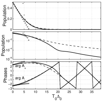
Figure 5: Asymptotic adiabatic state population $P_{+}=\left|A_{+}\right|^{2}$ [upper frame; numerics (full lines), perturbation theory for large detuning (50) (dotted lines), for small detuning (76) (squared lines) and approximate formula (86)], the same with semi-log scale plot (middle frame), and phases $\arg A_{-}$ and $\arg A_{+}$ [lower frame; numerics (full lines), using approximations (49) (dotted lines), (75) (squared lines) and (85)] as functions of $T_{0}\Delta_{0}$ for the rising of the coupling with $n=2$ and $T_{0}\Omega_{0}=100$ (calculated at the asymptotic time $\tau=3T_{0}$).

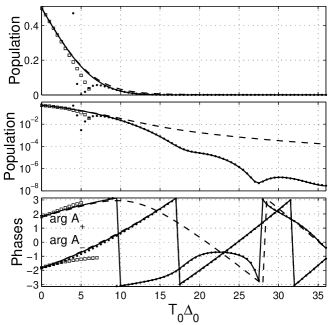
Figure 6: Same as Fig. 5 for the rising of the coupling with $n=3$ (calculated at $\tau=2.5T_{0}$).

For a smooth lifting of degeneracy [with a coupling such as exponential (11) or Gaussian coupling (13)], the terms of type $S$ (60) are all zero. Only an exponentially small term contributes to the lifting of quasi-degeneracy for large detuning.

VII Perturbation theory for small detuning

For small detuning $T_{0}\Delta_{0}\ll 1$ it is convenient to apply perturbation theory with $\varepsilon=T_{0}\Delta_{0}$ in the Landau-Zener basis as described below. The amplitudes $\phi_{LZ}(\tau)$ of the states in the Landau-Zener basis are obtained from the amplitudes of the bare states via the time-independent unitary transformation $\mathsf{S}$:

$$\phi_{LZ}(\tau)\equiv\left[\begin{array}[]{c}Z_{-}(\tau)\\ Z_{+}(\tau)\end{array}\right]=\mathsf{S}^{\dagger}\phi(\tau),$$ (64)

with

$$\mathsf{S}=\frac{1}{\sqrt{2}}\left[\begin{array}[]{cc}1&1\\ -1&1\end{array}\right],$$ (65)

giving the Landau-Zener Hamiltonian

$$\mathsf{H}_{LZ}(\tau) \equiv\mathsf{S}^{\dagger}\mathsf{H}(\tau)\mathsf{S}$$ (66a)

$$=\frac{\hbar}{2}\left[\begin{array}[]{cc}-\Omega(\tau)&-\Delta_{0}\\ -\Delta_{0}&\Omega(\tau)\end{array}\right],$$ (66d)

associated to the Schrödinger equation

$$i\hbar\frac{\partial\phi_{LZ}}{\partial\tau}(\tau)=T_{0}\mathsf{H}_{LZ}(\tau)\phi_{LZ}(\tau),$$ (67)

and the initial conditions

$$Z_{\pm}(\tau_{i})=\frac{1}{\sqrt{2}},$$ (68)

since one starts with $A_{-}(\tau_{i})=B_{-}(\tau_{i})=1,$ $A_{+}(\tau_{i})=B_{+}(\tau_{i})=0$ [see Eq. (22)]. The zero order of perturbation theory gives

$$Z_{\pm}^{(0)}(\tau)=\frac{1}{\sqrt{2}}e^{\mp i\zeta(\tau)}$$ (69)

where $\zeta(\tau)$ is the instantaneous dimensionless pulse half-area

$$\zeta(\tau)=\frac{T_{0}}{2}\int_{\tau_{i}}^{\tau}\Omega(\tau^{\prime})d\tau^{\prime}.$$ (70)

The first order contribution reads

$$\varepsilon Z_{\pm}^{(1)}(\tau)=i\frac{T_{0}\Delta_{0}}{2\sqrt{2}}e^{\mp i\zeta(\tau)}\int_{\tau_{i}}^{\tau}d\tau^{\prime}e^{\pm 2i\zeta(\tau^{\prime})},$$ (71)

leading to the first order solution

$$Z_{\pm}(\tau)\approx Z_{\pm}^{(0)}(\tau)+\varepsilon Z_{\pm}^{(1)}(\tau).$$ (72)

For large times $\tau\rightarrow+\infty$, $\mathsf{H}_{LZ}(\tau)$ becomes diagonal and $\phi_{LZ}(\tau)$ asymptotically coincides with $\phi_{A}(\tau)$, which gives at first order:

$$A_{\pm}(\tau)\rightsquigarrow\frac{1}{\sqrt{2}}e^{\mp i\zeta(\tau)}\left(1+i\frac{T_{0}\Delta_{0}}{2}\int_{\tau_{i}}^{\tau}d\tau^{\prime}e^{\pm 2i\zeta(\tau^{\prime})}\right).$$ (73)

The transition probability at first order can be thus written as

$$P_{+}(\tau)\rightsquigarrow\frac{1}{2}\left[1-T_{0}\Delta_{0}\int_{\tau_{i}}^{\tau}d\tau^{\prime}\sin\left(2\zeta(\tau^{\prime})\right)\right].$$ (74a)

For the power law rising coupling, one thus obtains for large times $$\tau\rightarrow+\infty$$

$$A_{\pm}(\infty)\approx\frac{1}{\sqrt{2}}e^{\mp i\zeta(\tau)}\left[1+\frac{T_{0}\Delta_{0}}{2}\left(\mp K_{n}+iL_{n}\right)\right]$$ (75)

and

$$P_{+}(\infty)\approx\frac{1}{2}\left(1-T_{0}\Delta_{0}K_{n}\right)$$ (76)

with

$$\zeta(\tau)=\frac{T_{0}\Omega_{0}}{2}\frac{\tau^{n+1}}{n+1},$$ (77)

$$K_{n} =\left(\frac{n+1}{T_{0}\Omega_{0}}\right)^{\frac{1}{n+1}}\int_{0}^{\infty}ds\sin\left(s^{n+1}\right)$$ (78a)

$$=\left(\frac{1}{T_{0}\Omega_{0}}\right)^{\frac{1}{n+1}}\frac{\sqrt{\pi}}{\left[2\left(n+1\right)\right]^{n/\left(n+1\right)}}\frac{\Gamma\left(\frac{n+2}{2\left(n+1\right)}\right)}{\Gamma\left(\frac{2n+1}{2\left(n+1\right)}\right)}$$ (78b)

and

$$L_{n} =\left(\frac{n+1}{\Omega_{0}T_{0}}\right)^{\frac{1}{n+1}}\int_{0}^{\infty}ds\cos\left(s^{n+1}\right)$$ (79a)

$$=\left(\frac{1}{T_{0}\Omega_{0}}\right)^{\frac{1}{n+1}}\frac{\sqrt{\pi}}{\left[2\left(n+1\right)\right]^{n/\left(n+1\right)}}\frac{\Gamma\left(\frac{1}{2\left(n+1\right)}\right)}{\Gamma\left(\frac{n}{2\left(n+1\right)}\right)}$$ (79b)

$$=\frac{\sin\left(\frac{\pi}{2}\frac{n+2}{n+1}\right)}{\sin\left(\frac{\pi}{2}\frac{2n+1}{n+1}\right)}K_{n}.$$ (79c)

For $$n=1 K_{1}=\sqrt{\pi/T_{0}\Omega_{0}}/2=\sqrt{\pi/2}\omega/T_{0}\Delta_{0}$$, one has in particular and

$$P_{+}(\infty)\approx\frac{1}{2}\left(1-\sqrt{\frac{\pi}{2}}\omega\right),$$ (80)

with $\omega$ given by Eq. (35), which is recovered from the exact asymptotic solution (33) in the limit of small detuning.

Figure 5 shows the transition probability and the phases for $n=2$ obtained with the preceding formulas. The agreement is good until $T_{0}\Delta_{0}\approx 5$. The two perturbative formulas for small and large detunings almost match for the probability. Only a small region of intermediate detuning is not covered by either approximation.

In the case of the exponential coupling (11) with $\tau_{i}\rightarrow-\infty$, we obtain, using the variable $x=T_{0}\Delta_{0}\exp(\tau)$, in the asymptotic limit $\tau\rightarrow\infty$:

$$P_{+}(\infty) \approx\frac{1}{2}\left(1-T_{0}\Delta_{0}\int_{0}^{\infty}dx\frac{\sin x}{x}\right)$$ (81a)

$$=\frac{1}{2}\left(1-\frac{\pi}{2}T_{0}\Delta_{0}\right),$$ (81b)

which coincides with the exact asymptotic result (41) in the limit of small detuning.

For the Gaussian coupling (13), one obtains with the asymptotic limit taken at $\tau=0$:

$$P_{+}(0)=\frac{1}{2}\left[1-G(T_{0}\Omega_{0})T_{0}\Delta_{0}\right]$$ (82)

with

$$G(x)=\int_{-\infty}^{0}d\tau\sin\left[\frac{\sqrt{\pi}}{2}x\left(1+\text{erf}\left(\tau\right)\right)\right].$$ (83)

The function $G(x)$ is shown in Fig. 7. It oscillates less and less for larger $x$, and goes very slowly to 0. We are interested in the adiabatic limit $x\equiv T_{0}\Omega_{0}\gg 1$, where $G(x)$ depends weakly on $x$. This allows us to conclude that, in the limit of small detunings and large $T_{0}\Omega_{0}$, the population transfer is quite robust with respect to the peak amplitude: $\lim_{T_{0}\Omega_{0}\gg 1}\left|dP_{+}(0)/d\left(T_{0}\Omega_{0}\right)\right|\ll 1$. Already for $T_{0}\Omega_{0}\sim 10$, we have $\left|dP_{+}(0)/d\left(T_{0}\Omega_{0}\right)\right|<0.05\times T_{0}\Delta_{0}$. Moreover we can remark that it is a bit more robust with respect to the detuning than the exponentially rising case: for $T_{0}\Omega_{0}\sim 10$, we have $\left|dP_{+}(0)/d\left(T_{0}\Delta_{0}\right)\right|<0.3$ (to be compared with the exponentially rising, where we have the constant value $\left|dP_{+}(0)/dT_{0}\Delta_{0}\right|=\pi/4\approx 0.79$).

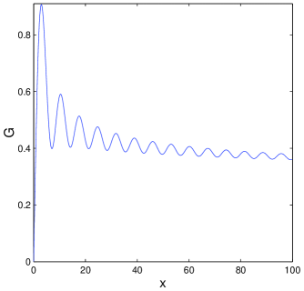
Figure 7: Function $G(x)$ as defined in Eq. (83) involved in the population transfer (82) for the Gaussian coupling and small detunings.

VIII Approximate formula for arbitrary detuning

The result (76) for small detuning suggests to extend for arbitrary $n$ the exact results of $n=1$ [Eqns (32) to (39)] replacing in these formulae $\omega$ by $\omega_{n}$:

$$\omega_{n} \equiv\sqrt{\frac{2}{\pi}}K_{n}T_{0}\Delta_{0}$$ (84a)

$$=T_{0}\Delta_{0}\left(\frac{1}{T_{0}\Omega_{0}}\right)^{\frac{1}{n+1}}\frac{\sqrt{2}}{\left[2(n+1)\right]^{n/\left(n+1\right)}}\frac{\Gamma\left(\frac{n+2}{2\left(n+1\right)}\right)}{\Gamma\left(\frac{2n+1}{2\left(n+1\right)}\right)}.$$ (84b)

Asymptotic analysis allows us to extend the phases as follows: For large $$T_{0}\Delta_{0} S_{n} n T_{0}\Delta_{0}$$, we take into account the contribution (60) [which gives the additional prefactor in Eq. (89)]; for small , we have used (75) [which gives the additional sine ratio in Eq. (88)]. We finally obtain

$$A_{n,\pm}(\tau)\rightsquigarrow\sqrt{p_{n,\pm}}\ e^{\mp i\left(\chi_{n,\pm}+\eta_{n}(\tau)\right)}$$ (85)

with the transition probabilities

$$p_{n,\pm} \equiv\left|A_{n,\pm}\right|^{2}=\frac{1}{2}\left(1\mp\sqrt{1-e^{-\pi\omega_{n}^{2}}}\cos\varphi_{n}\right),$$ (86)

$$\varphi_{n} =\arg\Gamma\left(1-i\frac{\omega_{n}^{2}}{4}\right)-\arg\Gamma\left(\frac{1}{2}-i\frac{\omega_{n}^{2}}{4}\right)+\frac{\pi}{4},$$ (87)

and the phases

$$\chi_{n,-} =\frac{\sin\left(\frac{\pi}{2}\frac{2n+1}{n+1}\right)}{\sin\left(\frac{\pi}{2}\frac{n+2}{n+1}\right)}\chi_{n,0}+\arg\left(a_{n}+b_{n}e^{i\varphi_{n}}\right),$$ (88)

$$\chi_{n,+} =\chi_{n,0}+n\arg\left(a_{n}-b_{n}e^{i\varphi_{n}}\right),$$ (89)

$$\chi_{n,0} =\arg\Gamma\left(\frac{1}{2}-i\frac{\omega_{n}^{2}}{4}\right)-\frac{\omega_{n}^{2}}{4}\left(1-\ln\frac{\omega_{n}^{2}}{4}\right),$$ (90)

$$a_{n} =\frac{1}{\sqrt{2}}\sqrt{1+e^{-\pi\omega_{n}^{2}/2}},\ b_{n}=\frac{1}{\sqrt{2}}\sqrt{1-e^{-\pi\omega_{n}^{2}/2}},$$ (91)

$$\eta_{n}(\tau) =\frac{T_{0}}{2}\int_{0}^{\tau}\sqrt{\Delta_{0}^{2}+\Omega_{0}^{2}\tau^{2n}}d\tau.$$ (92)

It is remarkable that the amplitude depends only on $\omega_{n}$ (and also on the dynamical phase $\eta_{n}(\tau)$ and $n$). This quantity gives the scaling of the lifting of degeneracy. Figure 5 shows the good accuracy of formula (85) for any detuning for $n=2$. Only a logarithmic scale shows that the probablities are not as precise as perturbation theory for large detuning. Figure 6 displays the result for $n=3$. The populations $p_{2,\pm}$ and the phase $\arg A_{2,-}$ are quite good for any detuning. The phase $\arg A_{2,+}$ is well reproduced for $T_{0}\Delta_{0}<10$.

One can remark that, as a function of the detuning, for $T_{0}\Delta_{0}<5$ , the phases change less fast than the populations. Thus the phases are more robust than the populations with respect to the detuning..

IX Application to the lineshape of the resonant excitation by strong pulses

In this section we apply the preceding formulation to calculate the transition probability after a pulse excitation of bell-like shape and of large area

$$\mathcal{A}\equiv 2\zeta(\tau_{f})=T_{0}\int_{\tau_{i}}^{\tau_{f}}\Omega(\tau^{\prime})d\tau^{\prime}\gg 1$$ (93)

to allow one to apply the preceding analysis for which a time where dynamics is adiabatic must occur. We consider the secant hyperbolic pulse coupling and recover the well-known Rosen-Zener formula. Discontinuous derivative endings are next considered with the examples of truncated trig-pulses. We study the lineshape, i.e. the transition probability as a function of the detuning.

We consider the initial condition $B_{-}(\tau_{i})=1$, $B_{+}(\tau_{i})=0$.

IX.1 General calculation

Between the lifting and creation of quasi-degeneracy, the pulse is assumed to be an arbitrary smooth function between $\tau_{i}$ and $\tau_{f}$, sufficiently far from zero to avoid intermediate creation of degeneracy. The time evolution operator can thus be decomposed as:

$$U(\tau_{f},\tau_{i}) = \left[\begin{array}[]{cc}U_{11}(\tau_{f},\tau_{i})&U_{12}(\tau_{f},\tau_{i})\\ -\left[U_{12}(\tau_{f},\tau_{i})\right]^{\ast}&\left[U_{11}(\tau_{f},\tau_{i})\right]^{\ast}\end{array}\right]$$ (94c)

$$= \mathsf{R}(\tau_{f})U_{c}(\tau_{f},\tau_{2})U_{a}(\tau_{2},\tau_{1})U_{\ell}(\tau_{1},\tau_{i})\mathsf{R}^{\dagger}(\tau_{i}),$$ (94d)

where [see Eqs. (130), (156)]

$$U_{\ell}(\tau_{1},\tau_{i})=\left[\begin{array}[]{cc}U_{A+}^{11}(\tau_{1},\tau_{i})&U_{A+}^{12}(\tau_{1},\tau_{i})\\ -\left[U_{A+}^{12}(\tau_{1},\tau_{i})\right]^{\ast}&\left[U_{A+}^{11}(\tau_{1},\tau_{i})\right]^{\ast}\end{array}\right]$$ (95a)

and [see Eq. (182)]

$$U_{c}(\tau_{f},\tau_{2})=\left[\begin{array}[]{cc}U_{A+}^{11}(\tau_{2}^{\prime},\tau_{f})&-\left[U_{A+}^{12}(\tau_{2}^{\prime},\tau_{f})\right]^{\ast}\\ U_{A+}^{12}(\tau_{2}^{\prime},\tau_{f})&\left[U_{A+}^{11}(\tau_{2}^{\prime},\tau_{f})\right]^{\ast}\end{array}\right],$$ (96a)

with $$\tau_{2}^{\prime}=-\tau_{2}+2\tau_{f} \tau_{2}^{\prime}=-\tau_{2}$$ for the power law falling and for a smooth (exponential or Gaussian) falling, are associated to the evolution operators of respectively lifting and creation of degeneracy in the adiabatic basis, and

$$U_{a}(\tau_{2},\tau_{1})\mathbf{=}\left[\begin{array}[]{cc}e^{i\left[\eta_{d}(\tau_{2})-\eta_{d}(\tau_{1})\right]}&0\\ 0&e^{-i\left[\eta_{d}(\tau_{2})-\eta_{d}(\tau_{1})\right]}\end{array}\right],$$ (97)

with

$$\eta_{d}(\tau)=\frac{T_{0}}{2}\int_{0}^{\tau}d\tau\sqrt{\Delta_{0}^{2}+\Omega^{2}(\tau)},$$ (98)

is associated to the adiabatic evolution between. Since the adiabatic states coincide with the bare states at early and late times, we have $\mathsf{R}^{\dagger}(\tau_{i})=\mathsf{R}(\tau_{f})=\openone$. The amplitudes of the bare states at the end of the pulse read thus

$$B_{-}(\tau_{f}) = U_{11}(\tau_{f},\tau_{i}),$$ (99a)

$$B_{+}(\tau_{f}) = -\left[U_{12}(\tau_{f},\tau_{i})\right]^{\ast}.$$ (99b)

IX.2 Secant hyperbolic pulse

The coupling reads in this case

$$\Omega(\tau)=\Omega_{0}\sec\text{h}(\tau)\equiv\frac{\Omega_{0}}{\cosh(\tau)}$$

with $\tau_{i}\rightarrow-\infty$ and $\tau_{f}\rightarrow+\infty$, whose asymptotics rise and fall exponentially: $\Omega(\tau)\rightsquigarrow 2\Omega_{0}\exp(\mp\tau)$ for $\tau\rightarrow\pm\infty$. We thus calculate $B_{+}(\tau_{f})$ applying Eqs. (99b) and (94d), and using the asymptotic result [Eqs. (175)], which requires $s(\tau_{1})\equiv T_{0}\int_{-\infty}^{\tau_{1}}\Omega(\tau)d\tau=T_{0}\Omega_{0}\exp(\tau_{1})\gg\varpi\equiv T_{0}\Delta_{0}$ (with $\tau_{1}<0$) for the lifting of quasi-degeneracy (see Appendix B) and $T_{0}\Omega_{0}\exp(-\tau_{2})\gg T_{0}\Delta_{0}$ (with $\tau_{2}>0$) for the creation of quasi-degeneracy. These two conditions are satisified for $\Omega_{0}\gg\Delta_{0}$.

In this limit, we obtain

$$B_{+}(\infty) \rightsquigarrow -i\frac{\sin\left[T_{0}\int_{-\infty}^{+\infty}\Omega(\tau)d\tau/2\right]}{\cosh\left(\pi T_{0}\Delta_{0}/2\right)}$$ (100a)

$$= -i\frac{\sin\left(\pi T_{0}\Omega_{0}/2\right)}{\cosh\left(\pi T_{0}\Delta_{0}/2\right)},$$ (100b)

$$B_{-}(\infty) \rightsquigarrow e^{2i\xi}[\cos\left(\pi T_{0}\Omega_{0}/2\right)$$ (100c)

$$+i\sin\left(\pi T_{0}\Omega_{0}/2\right)\tanh(\pi T_{0}\Delta_{0}/2)]$$

with $$\xi$$ defined in (Eq. 44), which allows to recover the well-known Rosen-Zener formula RosenZener

$$\left|B_{+}(\infty)\right|^{2}=\frac{\sin^{2}\left(T_{0}\Omega_{0}\pi/2\right)}{\cosh^{2}\left(\pi T_{0}\Delta_{0}/2\right)}\equiv P_{RZ},$$ (101)

which is exact for any $\Omega_{0}$ and $\Delta_{0}$. Note also that the phase of $B_{+}(\infty)$ is also exact, but that the phase of $B_{-}(\infty)$ is only approximatively valid for small $T_{0}\Delta_{0}$.

IX.3 Truncated pulses of linear endings

We assume that the pulse starts and ends with linear rising and falling around respectiveley $\tau_{i}=0$ and $\tau_{f}=\tau_{p}\gg 1:$

$$\Omega(\tau) \sim \Omega_{0}\tau,\quad 1>\tau\geq 0,$$ (102a)

$$\Omega(\tau) \sim \Omega_{0}\left(\tau_{p}-\tau\right),\quad\tau_{p}-1<\tau\leq\tau_{p}$$ (102b)

with the discontinuous first derivative

$$\Omega_{0}=\left.\frac{d\Omega}{d\tau}\right|_{\tau=0}=-\left.\frac{d\Omega}{d\tau}\right|_{\tau=\tau_{p}},$$ (103)

such that the lifting (resp. creation) of degeneracy occurs during the linear rising (resp. falling) of the pulse. We assume $\tau_{1}\sim 1,$ $\tau_{2}\sim\tau_{f}-1$ in Eq. (94d). We obtain the amplitudes of the bare states at the end of the pulse

$$B_{-}(\tau_{p}) = p_{-}e^{i\left(2\chi_{-}+\eta_{d}(\tau_{p})\right)}+p_{+}e^{-i\left(2\chi_{+}+\eta_{d}(\tau_{p})\right)}$$ (104a)

$$= \cos\psi\cos\varphi+\sin\psi$$ (104c)

$$\times\left(i\sqrt{1-e^{-\pi\omega^{2}}}+e^{-\pi\omega^{2}/2}\sin\varphi\right)$$

$$B_{+}(\tau_{p}) = -2i\sqrt{p_{+}p_{-}}\sin\left(\chi_{-}+\chi_{+}+\eta_{d}(\tau_{p})\right)$$ (104d)

$$= i\left(\cos\psi\sin\varphi-e^{-\pi\omega^{2}/2}\sin\psi\cos\varphi\right)$$ (104e)

with $$p_{\pm} \chi_{\pm}$$ and respectively defined in Eqs. (33) and (37), and

$$\omega^{2} = \frac{\left(T_{0}\Delta_{0}\right)^{2}}{2T_{0}\Omega_{0}}=\frac{T_{0}\Delta_{0}^{2}}{2}\left(\left.\frac{d\Omega}{d\tau}\right|_{\tau=0}\right)^{-1},$$ (105)

$$\varphi = \arg\Gamma\left(1-i\frac{\omega^{2}}{4}\right)-\arg\Gamma\left(\frac{1}{2}-i\frac{\omega^{2}}{4}\right)+\frac{\pi}{4},$$ (106)

$$\psi = \eta_{d}(\tau_{p})-\frac{1}{2}\omega^{2}\left(1-\ln\frac{\omega^{2}}{4}\right)+\frac{\pi}{4},$$ (107)

$$+\arg\Gamma\left(\frac{1}{2}-i\frac{\omega^{2}}{4}\right)+\arg\Gamma\left(1-i\frac{\omega^{2}}{4}\right).$$

Thus the lineshape $\left|B_{+}(\tau_{p})\right|^{2}$ is determined only by the dynamical phase and the first discontinuous derivative of the pulse.

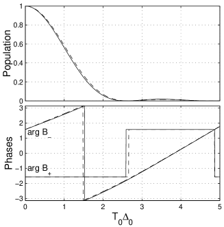
Figure 8: Lineshape $\left|B_{+}(\tau_{p})\right|^{2}$ [upper frame; numerics (full lines) and using approximate formula (104e)], and phases $\arg A_{-}$ and $\arg A_{+}$ as functions of $T_{0}\Delta_{0}$ for the trig-pulse (108) and $T_{0}\Omega_{0}=\pi/2$.

Figure 8 shows an example of the lineshape, accompanied with the phases, for the trig-pulse

$$\Omega(\tau)=\Omega_{0}\sin\tau,\quad 0\leq\tau\leq\pi,$$ (108)

giving $\mathcal{A}=2T_{0}\Omega_{0}.$ We have chosen $T_{0}\Omega_{0}=\pi/2$, i.e. a ”$\pi$-pulse” which induces a complete population transfer for $\Delta_{0}=0$ in this model. One can see that even for this $\pi$-pulse for which the condition of large area $\mathcal{A}\gg 1$ is valid only very roughly, the numerical and analytical result (104) are very close. One can remark that as shown by Eq. (104e), the phase of $B_{+}(\tau_{p})$ is $\pm\pi/2$ and does not depend on the dynamical phase.

IX.4 Truncated pulses of power law endings

We assume that the pulse starts and ends with power law rising and falling around $\tau_{i}=0$ and $\tau_{f}=\tau_{p}\gg 1:$

$$\Omega(\tau) \sim \Omega_{0}\tau^{n},\quad 1>\tau\geq 0,$$ (109a)

$$\Omega(\tau) \sim \Omega_{0}\left(\tau_{p}-\tau\right)^{n},\quad\tau_{p}-1<\tau\leq\tau_{p}$$ (109b)

with the discontinuous $$n^{\text{th}}$$ derivative

$$\Omega_{0}=\frac{1}{n!}\left.\frac{d^{n}\Omega}{d\tau^{n}}\right|_{\tau=0}.$$ (110)

Using the generalization of the results for $n>1$ of the preceding Section, we obtain

$$B_{+}(\tau_{p}) = -2i\sqrt{p_{+}p_{-}}\sin\left(\chi_{-}+\chi_{+}+\eta_{d}(\tau_{p})\right)$$ (111a)

$$B_{-}(\tau_{p}) = p_{-}e^{i\left(2\chi_{-}+\eta_{d}(\tau_{p})\right)}+p_{+}e^{-i\left(2\chi_{+}+\eta_{d}(\tau_{p})\right)}$$ (111b)

with $$p_{\pm} \chi_{\pm} \eta_{d} P_{+}=\left|B_{+}(\tau_{p})\right|^{2} n^{\text{th}}$$, and respectively defined in Eqs. (86), (88), (89) and (98). Thus the lineshape is determined only by the dynamical phase and the discontinuous derivative of the pulse.

This allows to calculate approximately the lineshape for a trig-pulse

$$\Omega(\tau)=\Omega_{0}\sin^{n}\tau,\quad 0\leq\tau\leq\pi,$$ (112)

where $\left.\frac{d^{n}\Omega}{d\tau^{n}}\right|_{\tau=0}=\Omega_{0}\tau^{n}$.

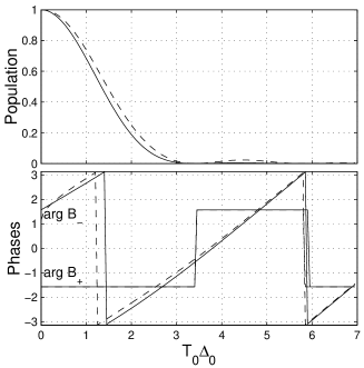
Figure 9: Same as Fig. 8 for the trig-pulse (113) and $T_{0}\Omega_{0}=2$ ($\pi$-pulse).

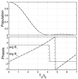
Figure 10: Same as Fig. 9 for $T_{0}\Omega_{0}=6$ ($3\pi$-pulse).

Figure 9 and 10 give two examples of the lineshape, accompanied with the phases, for the trig-pulse

$$\Omega(\tau)=\Omega_{0}\sin^{2}\tau,\quad 0\leq\tau\leq\pi,$$ (113)

giving $\mathcal{A}=T_{0}\Omega_{0}\pi/2$, respectively in ”$\pi$-pulse” and ”3$\pi$-pulse” conditions. The numerical and analytical results are quite close.

X Application to Half-SCRAP

It has been shown recently that two delayed pulsed lasers in an adiabatic regime can be used to yield a coherent superposition of states. This process has been named Half SCRAP HSCRAP . It permits to create at the end of the interaction a coherent superposition of states, whose amplitudes do not depend on the dynamical phases and are thus robust with respect to the field amplitudes. One uses two delayed lasers: a pump one-photon resonant laser and an off-resonant Stark laser which allows to dynamically shift the levels. The effective Hamiltonian is of the form (7) in the basis of the dressed energies $\left|-;0\right\rangle$ (state $\left|-\right\rangle$ dressed by 0 photon) and $\left|+;-1\right\rangle$ (state $\left|+\right\rangle$ dressed by -1 photon), that are degenerate for the exact one-photon resonance ($\Delta=0$) when $\Omega=0$.

We can interpret the process using the topology of the eigenenergy surfaces as functions of the parameters $\Omega$ and $\Delta$, combined with a local analysis of lifting (resp. creation) of quasi-degeneracy near the start (resp. end) of the process.

The time dependence of the effective detuning $\Delta(t)=\Delta_{0}+S(t)$ is only due to Stark shifts which are induced by the laser pulses. The process can be described by the diagram of the two surfaces

$$\lambda_{\pm}(\Omega,\Delta)=\pm\frac{\hbar}{2}T_{0}\sqrt{\Omega^{2}+\Delta^{2}}$$ (114)

which represent the eigenenergies as functions of the instantaneous effective Rabi frequency $\Omega$ and detuning $\Delta$ (see Fig. 11). The associated eigenvectors can be written as

$$\left|\Phi_{-}\right\rangle=\left[\begin{array}[]{c}\cos\theta\\ -\sin\theta\end{array}\right],\quad\left|\Phi_{+}\right\rangle=\left[\begin{array}[]{c}\sin\theta\\ \cos\theta\end{array}\right]$$ (115)

with

$$\tan 2\theta=\frac{\Omega}{\Delta},\quad 0\leq\theta<\pi/2.$$ (116)

The surfaces display a conical intersection for $\Omega=0,\Delta=0$ induced by the crossing of the lines corresponding to states $\left|-;0\right\rangle$ and $\left|+;-1\right\rangle$ for $\Omega=0$ and various $\Delta$. We study a quasi-resonant process starting (and ending) close to this conical intersection.

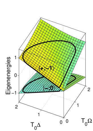
Figure 11: Surfaces of eigenenergies (114) as functions of $T_{0}\Omega$ and $T_{0}\Delta$ (considered both positive). The lines in the plane $\Omega=0$, connected to the respective lower and upper surfaces, characterize the states respectively $\left|-;0\right\rangle$ and $\left|+;-1\right\rangle$. One example of paths involving a lifting of quasi-degeneracy is drawn.

One essential point is that the result of the lifting (or creation) of quasi-degeneracy depends on the direction of the lifting (or creation). We can characterize two particular directions: In the $\Delta$ direction with $\Omega=0$, we have $\theta=0$, which means that the lifting and creation of degeneracy occur trivially along a unique surface:

$$\left|-;0\right\rangle = \left|\Phi_{-}\right\rangle,$$ (117a)

$$\left|+;-1\right\rangle = \left|\Phi_{+}\right\rangle.$$ (117b)

In the $$\Omega \Delta=0 \theta=\pi/4$$ direction with , we have , i.e

$$\left|-;0\right\rangle = \frac{1}{\sqrt{2}}\left(\left|\Phi_{+}\right\rangle+\left|\Phi_{-}\right\rangle\right),$$ (118a)

$$\left|+;-1\right\rangle = \frac{1}{\sqrt{2}}\left(\left|\Phi_{+}\right\rangle-\left|\Phi_{-}\right\rangle\right),$$ (118b)

which implies a lifting of degeneracy occuring along the lower and upper surfaces with an equal sharing ($$1/2 \Delta \Omega$$ if we consider the probabilities). In other directions, the lifting of degeneracy results from a competition between the parameters and and will give a mixing of the two surfaces with non equal sharing in general.

The $\Omega$ direction with an arbitrary $\Delta$ will result in a lifting of quasi-degeneracy as studied in the preceding sections.

The inverse process of creation of degeneracy also depends on the direction in which the eigenstates involved in the dynamics arrive into the degeneracy. In the $\Omega$ direction with $\Delta=0$, we have

$$\left|\Phi_{-}\right\rangle = \frac{1}{\sqrt{2}}\left(\left|-;0\right\rangle-\left|+;-1\right\rangle\right)$$ (119a)

$$\left|\Phi_{+}\right\rangle = \frac{1}{\sqrt{2}}\left(\left|-;0\right\rangle+\left|+;-1\right\rangle\right),$$ (119b)

To obtain a coherent superposition of states, we have two possibilities:

(i) first lifting of degeneracy in the $\Delta$ direction with $\Omega=0$ [according to Eq. (117a)] giving one single dressed state involved in the dynamics; next adiabatic following on this dressed state (along the lower surface) and finally creation of quasi-degeneracy in the $\Omega$ direction [according to Eq. (119a) for the case of exact resonance $\Delta=0$];

(ii) first lifting of quasi-degeneracy in the $\Omega$ direction [according to Eq. (118a) for the case of exact resonance $\Delta=0$] giving two dressed states involved in the dynamics; next independent adiabatic following on these two dressed states (along both the lower and upper surfaces) and finally creation of degeneracy in the $\Delta$ direction with $\Omega=0$ [according to Eq (117)].

These two cases are produced by two following different sequences of pulses: respectively (i) first the Stark pulse and next the pump pulse (referred to as Stark-pump sequence), (ii) first the pump pulse and next the Stark pulse (referred to as pump-Stark sequence). (Both sequences require an overlapping of the two pulses to induce adiabatic following.)

The dynamical phases coming from these two different sequences are not identical. For the sequence Stark-pump at exact resonance $\Delta=0$, we start with the lifting of degeneracy $\left|\phi\left(t_{i}\right)\right\rangle=\left|\Phi_{-}\right\rangle$, followed by an adiabatic passage

$$\left|\phi\left(t\right)\right\rangle=\text{e}^{-\text{i}\int_{t_{i}}^{t}ds\lambda_{-}(s)/\hbar}\left|\Phi_{-}\right\rangle,$$ (120)

which leads at the final time $t_{f}$ to

$$\left|\phi\left(t_{f}\right)\right\rangle=\frac{1}{\sqrt{2}}\text{e}^{-\text{i}\int_{t_{i}}^{t_{f}}ds\lambda_{-}(s)/\hbar}\left(\left|-\right\rangle-e^{-i\omega t}\left|+\right\rangle\right)$$ (121)

(where a coherent state for the photon field has been considered.) For the sequence pump-Stark at exact resonance $\Delta=0$, we start with the lifting of degeneracy $\left|\phi\left(t_{i}\right)\right\rangle=\left(\left|\Phi_{+}\right\rangle+\left|\Phi_{-}\right\rangle\right)/\sqrt{2}$. The dynamics is next characterized by an adiabatic passage along each branch:

$$\left|\phi\left(t\right)\right\rangle=\frac{1}{\sqrt{2}}\left[\text{e}^{-\text{i}\int_{t_{i}}^{t}ds\lambda_{+}(s)/\hbar}\left|\Phi_{+}\right\rangle+\text{e}^{-\text{i}\int_{t_{i}}^{t}ds\lambda_{-}(s)/\hbar}\left|\Phi_{-}\right\rangle\right],$$ (122)

which leads at time $t_{f}$ to

$$\left|\phi\left(t_{f}\right)\right\rangle = \frac{1}{\sqrt{2}}\text{e}^{-\text{i}\int_{t_{i}}^{t_{f}}ds\lambda_{+}(s)/\hbar}$$ (123)

$$\times\left[e^{-i\omega t}\left|+\right\rangle+\text{e}^{\text{i}\int_{t_{i}}^{t_{f}}\frac{ds}{\hbar}\left(\lambda_{+}(s)-\lambda_{-}(s)\right)}\left|-\right\rangle\right].$$

Thus the two sequences (with exact one-photon resonance) lead to the same probabilities $1/2$ but with different phases. The pump-Stark sequence (123) leads to a coherent superposition of states with a (non-robust) phase difference $\int_{t_{i}}^{t_{f}}ds\left(\lambda_{+}(s)-\lambda_{-}(s)\right)/\hbar$, coinciding with the dynamical phase difference, in addition to the optical phase.

If one considers non exact one-photon resonance $\Delta\neq 0$, one obtains, by lifting of quasi-degeneracy, additional phases and amplitudes different from $1/\sqrt{2}$, that will depend on the shape of the pulses according to the analysis of the preceding sections. Fig. 12 gathers populations of different coherent superposition of states given by half-SCRAP for various pulse shapes. One can see that robustness with respect to the detuning is better for power law rising than for the exponential and Gaussian rising (better for small $n$ and large $\Omega_{0}$). Robustness with respect to the amplitude $\Omega_{0}$ is better for smoother rising (and better for the exponential rising, which is independent of $\Omega_{0}$, than for the Gaussian rising, which is weakly dependent on $\Omega_{0}$).

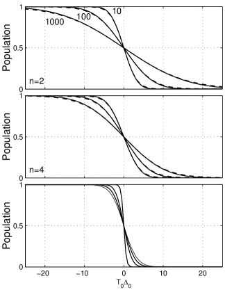
Figure 12: Half-SCRAP population transfers $P_{+}=\left|\langle+|\phi(t_{f})\rangle\right|^{2}$ for power rising of the pump laser (upper frame: $n=2$, middle frame: $n=4$) with respectively $T_{0}\Omega_{0}=1000,100,10$ from (upper) left to right (indicated close to each curve) [numerics: full lines, dashed lines: formulas (86)], and for Gaussian rising with respectively $T_{0}\Omega_{0}=1000,100,10$ and exponential rising from (upper) left to right (lower frame) as a function of $T_{0}\Delta_{0}$.

XI Conclusion

In this article, we have analyzed the dynamics associated with lifting of quasi-degeneracy with a constant detuning. This is the situation encountered for one-photon quasi-resonance. The dynamics becomes quite different for $n-$photon quasi-resonance in effective two-level models, which leads to an effective time-dependent detuning. Indeed, in this case the effective Hamiltonian is, in the basis $\left\{\left|-;0\right\rangle,\left|+;-n\right\rangle\right\}$, of the form

$$\mathsf{H}(\tau)\simeq\frac{\hbar}{2}\left[\begin{array}[]{cc}-\alpha\mathcal{E}^{2}(\tau)-\Delta&\beta\mathcal{E}^{n}(\tau)\\ \beta^{\ast}\mathcal{E}^{n}(\tau)&\alpha\mathcal{E}^{2}(\tau)+\Delta\end{array}\right]$$ (124)

with $\mathcal{E}(\tau)$ the field amplitude,$\ \alpha$ real (chosen positive), $\beta=\left|\beta\right|e^{i\varphi}$, and where only the leading second order (Stark shifts) have been kept in the diagonal. If $n=2$, all the terms of the matrix involving the field amplitude have the same order which complicates the lifting of quasi-degeneracy. If $\Delta=0$, we obtain the following lifting of degeneracy Guerin_PRA97 ; review

$$\left|-;0\right\rangle = \sin\theta\left|\Phi_{+}\right\rangle+\cos\theta\left|\Phi_{-}\right\rangle,$$ (125a)

$$\left|+;-n\right\rangle = e^{i\varphi}\cos\theta\left|\Phi_{+}\right\rangle-e^{i\varphi}\sin\theta\left|\Phi_{-}\right\rangle,$$ (125b)

with

$$\tan 2\theta=\frac{\left|\beta\right|}{\alpha},\quad 0\leq\theta<\pi/2.$$ (126)

If $n>2$, it is known that “one can approximately compensate the Stark shift”. This can be explained and extended as follows on the example for the rising of the pulse: we separate the dynamics following the different orders in $\mathcal{E}$ of the matrix: (i) the Stark shift at early times shifts the diagonal elements (i.e. the dressed states in an effective way) for small field amplitudes without transferring any population, and (ii) for larger field amplitudes, the coupling lifts the resulting quasi-degeneracy. This last step can be in principle analyzed by the tools presented in this article. Thus, by adjusting $\Delta$, it is possible to cancel almost completely or more generally partially the effect of the Stark shift, leading to an arbitrary (in probability) superposition of states. The complete cancellation is for example the key that permits to orient molecules by adiabatic passage (in that case the Stark shift is of exponential order) orient .

The analysis of the lifting of quasi-degeneracy is more complicated in the case $n=2$ since the Stark shifts and the lifting occur simultaneously, leading to a lifting of quasi-degeneracy with a time-dependent detuning. This requires the extension of the tools presented here.

The present analysis has allowed to recover the lineshape for secant hyperbolic pulses (Rosen-Zener formula) and to determine quite precisely the lineshape for trig-pulses. The lineshape for Gaussian pulses is to our knowledge an open question.

XII Acknowledgments

We acknowledge support by INTAS 99-00019 and from Conseil Régional de Bourgogne. LY thanks l’Université de Bourgogne for several stays as invited professor during which this work was accomplished.

Appendix A Exact solution for a linearly rising coupling

The linearly rising (resp. falling) coupling problem can be solved exaclty by expressing it as a Landau-Zener problem of finite duration, with a start (resp. end) at the avoided crossing, the so-called half Landau-Zener problem Vitanov . In terms of time evolution operators, we have to solve

$$i\hbar\frac{\partial}{\partial\tau}U(\tau,\tau_{0})=T_{0}\mathsf{H}(\tau)U(\tau,\tau_{0}),\quad U(\tau_{0},\tau_{0})=\openone$$ (127)

and in the adiabatic basis

$$i\hbar\frac{\partial}{\partial\tau}U_{A}(\tau,\tau_{0})=\mathsf{H}_{A}(\tau)U_{A}(\tau,\tau_{0}),\;U_{A}(\tau_{0},\tau_{0})=\openone$$ (128)

with

$$U_{A}(\tau,\tau_{0})=\mathsf{R}^{\dagger}(\tau)U(\tau,\tau_{0})\mathsf{R}(\tau_{0})$$ (129)

which can be written as

$$U_{A}(\tau,\tau_{0})=\left[\begin{array}[]{cc}U_{A}^{11}(\tau,\tau_{0})&U_{A}^{12}(\tau,\tau_{0})\\ -\left[U_{A}^{12}(\tau,\tau_{0})\right]^{\ast}&\left[U_{A}^{11}(\tau,\tau_{0})\right]^{\ast}\end{array}\right]$$ (130)

[property also true for $U(\tau,\tau_{0})$], since the Hamiltonian $\mathsf{H}(\tau)$ is of trace 0. ($\ast$ stands for the complex conjugate.)

We consider the linearly rising coupling

$$\Omega(\tau)=\left\{\begin{array}[]{c}\Omega_{0}\tau,\;\tau\geqslant 0\\ 0,\;\tau<0\end{array}\right.$$ (131)

starting  at $\tau=\tau_{i}=0$. We will denote $U_{A+}(\tau,\tau_{0})$ [resp. $U_{A-}(\tau,\tau_{0})$] the evolution operator asociated to the rising (resp. falling) of the coupling

A.1 Landau-Zener basis

The amplitudes $\phi_{D}(\tau)$ of the states in the Landau-Zener basis are obtained from the amplitudes of the bare states via the time-independent unitary transformation $\mathsf{S}$:

$$\phi_{LZ}(\tau)\equiv\left[\begin{array}[]{c}Z_{-}(\tau)\\ Z_{+}(\tau)\end{array}\right]=\mathsf{S}^{\dagger}\phi(\tau),$$ (132)

with

$$\mathsf{S}=\frac{1}{\sqrt{2}}\left[\begin{array}[]{cc}1&1\\ -1&1\end{array}\right],$$ (133)

giving the Landau-Zener Hamiltonian

$$\mathsf{H}_{LZ}(\tau) \equiv\mathsf{S}^{\dagger}\mathsf{H}(\tau)\mathsf{S}$$ (134a)

$$=\frac{\hbar}{2}\left[\begin{array}[]{cc}-\Omega(\tau)&-\Delta_{0}\\ -\Delta_{0}&\Omega(\tau)\end{array}\right].$$ (134d)

We introduce the dimensionless time variable

$$T(\tau)=\sqrt{\frac{T_{0}\Omega_{0}}{2}}\tau$$ (135)

that leads to the Schrödinger equation

$$i\hbar\frac{\partial\tilde{\phi}_{LZ}}{\partial T}(T) =\mathsf{\tilde{H}}_{LZ}(T)\tilde{\phi}_{LZ}(T),$$ (136a)

$$\tilde{\phi}_{LZ}(T) =\left[\begin{array}[]{c}\tilde{Z}_{-}(T)\\ \tilde{Z}_{+}(T)\end{array}\right]\equiv\phi_{LZ}(\tau)$$ (136d)

with the Hamiltonian

$$\mathsf{\tilde{H}}_{LZ}(T)=\hbar\left[\begin{array}[]{cc}-T&-\omega\\ -\omega&+T\end{array}\right],$$ (137)

the dimensionless coupling

$$\omega=\frac{T_{0}\Delta_{0}}{\sqrt{2T_{0}\Omega_{0}}}$$ (138)

and the initial conditions at time

$$T_{i}\equiv T(\tau_{i})=0.$$ (139)

A.2 Exact solution

The problem is reduced to the finite Landau-Zener model with a start at $T=T_{i}=0$. Using the results of Ref. Vitanov one can write the exact solution of this problem:

$$\tilde{\phi}_{LZ}(T)=U_{LZ}\mathbf{(}T,T_{i})\tilde{\phi}_{LZ}(T_{i})$$ (140)

with

$$U_{LZ}(T,T_{i})=\mathsf{S}^{\dagger}U(\tau,\tau_{i})\mathsf{S}$$ (141)

and the evolution operator

$$U_{LZ}\mathbf{(}T,T_{i})=\left[\begin{array}[]{cc}U_{LZ}^{11}\mathbf{(}T,T_{i})&U_{LZ}^{12}\mathbf{(}T,T_{i})\\ -\left[U_{LZ}^{12}\mathbf{(}T,T_{i})\right]^{\ast}&\left[U_{LZ}^{11}\mathbf{(}T,T_{i})\right]^{\ast}\end{array}\right],$$ (142)

whose matrix elements read

$$U_{LZ}^{11}(T,T_{i}) = \frac{\Gamma\left(1-\frac{1}{2}i\omega^{2}\right)}{\sqrt{2\pi}}\left[D_{i\omega^{2}/2}\left(T\sqrt{2}e^{-i\pi/4}\right)D_{-1+i\omega^{2}/2}\left(T_{i}\sqrt{2}e^{i3\pi/4}\right)\right.$$ (143a)

$$\left.+D_{i\omega^{2}/2}\left(T\sqrt{2}e^{i3\pi/4}\right)D_{-1+i\omega^{2}/2}\left(T_{i}\sqrt{2}e^{-i\pi/4}\right)\right],$$

$$U_{LZ}^{12}(T,T_{i}) = \frac{\Gamma\left(1-\frac{1}{2}i\omega^{2}\right)}{\omega\sqrt{\pi}}e^{i\pi/4}\left[D_{i\omega^{2}/2}\left(T\sqrt{2}e^{-i\pi/4}\right)D_{i\omega^{2}/2}\left(T_{i}\sqrt{2}e^{i3\pi/4}\right)\right.$$ (143b)

$$\left.-D_{i\omega^{2}/2}\left(T\sqrt{2}e^{i3\pi/4}\right)D_{i\omega^{2}/2}\left(T_{i}\sqrt{2}e^{-i\pi/4}\right)\right],$$

where $D_{\nu}\left(z\right)$ represents the parabolic cylinder function of order $\nu$ and argument $z$. Since in our case $T_{i}=0$ and using

$$D_{\nu}\left(0\right)=\frac{2^{\nu/2}\sqrt{\pi}}{\Gamma\left(\frac{1-\nu}{2}\right)},$$ (144)

we obtain

$$U_{LZ}^{11}(T,T_{i}) = \frac{\Gamma\left(1-\frac{1}{2}i\omega^{2}\right)2^{-1+i\omega^{2}/4}}{\Gamma\left(1-\frac{1}{4}i\omega^{2}\right)}\left[D_{i\omega^{2}/2}\left(T\sqrt{2}e^{-i\pi/4}\right)+D_{i\omega^{2}/2}\left(T\sqrt{2}e^{i3\pi/4}\right)\right]$$ (145a)

$$U_{LZ}^{12}(T,T_{i}) = \frac{2^{i\omega^{2}/4}e^{i\pi/4}\Gamma\left(1-\frac{1}{2}i\omega^{2}\right)}{\omega\Gamma\left(\frac{1}{2}-\frac{1}{4}i\omega^{2}\right)}\left[D_{i\omega^{2}/2}\left(T\sqrt{2}e^{-i\pi/4}\right)-D_{i\omega^{2}/2}\left(T\sqrt{2}e^{i3\pi/4}\right)\right]$$ (145b)

A.2.1 Asymptotics

We calculate the asymptotic expansion for the evolution matrix $U_{LZ}$ when the evolution is adiabatic, i.e. for $\tau\gtrsim 1$ and for $T_{0}\Omega_{0}\gg 1$ since we will consider intermediate or small detunings. We will thus determine the asymptotic expansion in the limit $T\gg 1$. Following Ref. Vitanov , we have the leading terms of the large-argument and large-order asymptotic expansion

$$D_{i\omega^{2}/2}\left(T\sqrt{2}e^{-i\pi/4}\right) \rightsquigarrow \cos\vartheta(T)\exp\left[\frac{\pi}{8}\omega^{2}+i\eta\right]$$ (146a)

$$D_{i\omega^{2}/2}\left(T\sqrt{2}e^{i3\pi/4}\right) \rightsquigarrow \cos\vartheta(T)\exp\left[-\frac{3\pi}{8}\omega^{2}+i\eta\right]+\frac{\omega\sqrt{\pi}}{\Gamma\left(1-\frac{1}{2}i\omega^{2}\right)}\sin\vartheta(T)\exp\left[-\frac{\pi}{8}\omega^{2}-i\left(\eta+\frac{\pi}{4}\right)\right]$$ (146b)

with

$$\tan 2\vartheta(T)=\frac{\omega}{T}=\frac{\Delta_{0}}{\Omega_{0}\tau}$$ (147)

i.e.

$$\vartheta(T)=\frac{\pi}{4}-\theta(\tau),$$ (148)

and

$$\eta=-\frac{\omega^{2}}{4}+\frac{\omega^{2}}{2}\ln\left[\frac{1}{\sqrt{2}}\left(T+\sqrt{\omega^{2}+T^{2}}\right)\right]+\frac{T}{2}\sqrt{\omega^{2}+T^{2}}.$$ (149)

This asymptotic expansion (146) has been checked numerically to be in fact valid when either $\omega$ or $T$ is large. This will allow us to use it for any detuning $\Delta_{0}$ in the adiabatic region, i.e. when $T\gg 1$. Moreover this asymptotic expansion is already a good approximation for $T\sim 3$. Using

$$\arg\left(\frac{\Gamma\left(1-\frac{1}{2}i\omega^{2}\right)}{\Gamma\left(1-\frac{1}{4}i\omega^{2}\right)}\right)=\arg\Gamma\left(\frac{1}{2}-\frac{1}{4}i\omega^{2}\right)-\frac{1}{2}\omega^{2}\ln 2,$$ (150)

$$\left|\Gamma\left(1-i\alpha\right)\right|=\sqrt{\frac{\pi\alpha}{\sinh\left(\pi\alpha\right)}},\qquad\alpha\in\mathbb{R},$$ (151)

and

$$\Gamma\left(z\right)\Gamma\left(z+1/2\right)=\frac{\sqrt{\pi}}{2^{2z-1}}\Gamma(2z),\qquad z\in\mathbb{C},$$ (152)

we obtain

$$U_{LZ}^{11}\mathbf{(}T,T_{i}) \rightsquigarrow ae^{i\eta_{1}(T)}\cos\vartheta(T)+be^{-i\eta_{2}(T)}\sin\vartheta(T)$$ (153a)

$$U_{LZ}^{12}\mathbf{(}T,T_{i}) \rightsquigarrow be^{i\eta_{2}(T)}\cos\vartheta(T)-ae^{-i\eta_{1}(T)}\sin\vartheta(T)$$ (153b)

with

$$\eta_{1}(T) = \widetilde{\eta}_{d}(T)-\frac{\omega^{2}}{4}\left(1-\ln\frac{\omega^{2}}{4}\right)+\arg\Gamma\left(\frac{1}{2}-\frac{1}{4}i\omega^{2}\right),$$ (154a)

$$\eta_{2}(T) = \widetilde{\eta}_{d}(T)-\frac{\omega^{2}}{4}\left(1-\ln\frac{\omega^{2}}{4}\right)+\frac{\pi}{4}+\arg\Gamma\left(1-\frac{1}{4}i\omega^{2}\right),$$ (154b)

$$\widetilde{\eta}_{d}(T) \equiv \int_{0}^{T}\sqrt{\omega^{2}+T^{2}}dT=\frac{T}{2}\sqrt{\omega^{2}+T^{2}}+\frac{\omega^{2}}{2}\ln\frac{T+\sqrt{\omega^{2}+T^{2}}}{\omega},$$ (154c)

$$= \eta_{d}(\tau)\equiv\frac{1}{\hbar}\int_{0}^{\tau}\lambda_{+}(\tau)d\tau$$ (154d)

$$a = \frac{1}{\sqrt{2}}\sqrt{1+e^{-\pi\omega^{2}/2}},\quad b=\frac{1}{\sqrt{2}}\sqrt{1-e^{-\pi\omega^{2}/2}},$$ (154e)

where $\eta_{d}(T)$ corresponds to the dynamical phase associated to the positive instantaneous eigenvalue $\sqrt{\omega^{2}+T^{2}}$ of the Landau-Zener Hamiltonian $\mathsf{\tilde{H}}_{LZ}(T)/\hbar$ of Eq. (137).

A.3 Time evolution operator for the adiabatic states

The evolution operator in the basis of the adiabatic states can be written as

$$U_{A+}(\tau,0)=\mathsf{R}^{\dagger}\left(\tau\right)\mathsf{S}U_{LZ}(T(\tau),0)\mathsf{S}^{\dagger}\mathsf{R}\left(0\right),$$ (155)

with $\mathsf{R}\left(0\right)=\openone$. Thus,

$$U_{A+}^{11}(\tau,0) \rightsquigarrow\frac{1}{\sqrt{2}}\left[ae^{i\eta_{1}(T(\tau))}+be^{i\eta_{2}(T(\tau))}\right],$$ (156a)

$$U_{A+}^{12}(\tau,0) \rightsquigarrow\frac{1}{\sqrt{2}}\left[-ae^{i\eta_{1}(T(\tau))}+be^{i\eta_{2}(T(\tau))}\right].$$ (156b)

Appendix B Exact solution for exponentially rising coupling

The case of exponentially rising and falling coupling can be solved analytically in terms of the Kummer functions. Here we give the asymptotics of the evolution operator in the adiabaticity region where the population of the eigenstates is time independent.

We consider the rising coupling

$$\Omega(\tau)=\Omega_{0}e^{\tau}$$ (157)

with the initial condition at $\tau_{i}\rightarrow-\infty$.

B.1 Evolution operator for the bare states

It is convenient to introduce the new variable Delos ; Delos2

$$s(\tau)=T_{0}\int_{-\infty}^{\tau}\Omega(\tau^{\prime})d\tau^{\prime}=T_{0}\Omega_{0}e^{\tau},$$ (158)

that corresponds to the partial dimensionless pulse area. In terms of this new variable, the Schrödinger equation reads

$$i\frac{\partial\tilde{\phi}}{\partial s}(s) =\frac{1}{2}\left[\begin{array}[]{cc}-\Theta\left(s\right)&1\\ 1&\Theta\left(s\right)\end{array}\right]\tilde{\phi}(s),$$ (159c)

$$\tilde{\phi}(s) =\left[\begin{array}[]{c}\tilde{B}_{-}(s)\\ \tilde{B}_{+}(s)\end{array}\right]\equiv\phi(\tau)=\left[\begin{array}[]{c}B_{-}(\tau)\\ B_{+}(\tau)\end{array}\right]$$ (159h)

where

$$\Theta\left(s\right)=\frac{\Delta\left[\tau\left(s\right)\right]}{\Omega\left[\tau\left(s\right)\right]}$$ (160)

is called the Stueckelberg variable. In our case $\Delta\left[\tau\left(s\right)\right]=\Delta_{0,}$ $\Omega\left[\tau\left(s\right)\right]=s/T_{0}$, i. e.

$$\Theta\left(s\right)=\frac{T_{0}\Delta_{0}}{s}.$$ (161)

The differential equation for $\tilde{B}_{-}(s)$ for an arbitrary function $\Theta\left(s\right)$ reads

$$\frac{d^{2}\tilde{B}_{-}}{ds^{2}}(s)=-\frac{1}{4}\left[-2i\dot{\Theta}(s)+\Theta(s)^{2}+1\right]\tilde{B}_{-}(s),$$ (162)

which gives for the exponential coupling

$$\frac{d^{2}\tilde{B}_{-}}{ds^{2}}(s)=-\frac{1}{4}\left[2i\frac{T_{0}\Delta_{0}}{s^{2}}+\frac{\left(T_{0}\Delta_{0}\right)^{2}}{s^{2}}+1\right]\tilde{B}_{-}(s).$$ (163)

One starts from the time $\tau_{i}$ going to $-\infty.$ It means that $s_{i}=T_{0}\Omega_{0}e^{\tau_{i}}$ goes to zero (positive). The general initial conditions for $\tilde{B}_{-}(s)$ are

$$\tilde{B}_{-}(s_{i}) =B_{-}(\tau_{i}),$$ (164a)

$$\frac{d\tilde{B}_{-}}{ds}(s_{i}) =\frac{1}{2i}\left(B_{+}(\tau_{i})-\frac{T_{0}\Delta_{0}}{s}B_{-}(\tau_{i})\right).$$ (164b)

We introduce the new function

$$C_{-}(s)=\tilde{B}_{-}(s)s^{-i\varpi/2}$$ (165)

with

$$\varpi=T_{0}\Delta_{0},$$ (166)

whose evolution equation is

$$\frac{d^{2}C_{-}}{ds^{2}}(s)+i\frac{\varpi}{s}\frac{dC_{-}}{ds}(s)+\frac{1}{4}C_{-}(s)=0.$$ (167)

The general initial conditions for $C_{-}(s)$ read

$$C_{-}(s_{i}) =B_{-}(\tau_{i})s_{i}^{-i\varpi/2},$$ (168a)

$$\frac{dC_{-}}{ds}(s_{i}) =\frac{1}{2i}B_{+}(\tau_{i})s_{i}^{-i\varpi/2}.$$ (168b)

Considering the particular initial condition $$B_{-}(\tau_{i})=1, B_{+}(\tau_{i})=0 U_{11}(\tau,\tau_{i})=B_{-}(\tau) U_{21}(\tau,\tau_{i})=B_{+}(\tau) U(\tau,\tau_{i}) U_{22}(\tau,\tau_{i})=U_{11}^{\ast}(\tau,\tau_{i}) U_{12}(\tau,\tau_{i})=-U_{21}^{\ast}(\tau,\tau_{i}) \mathsf{H}(\tau)$$ will give the components and of the evolution operator , which is enough to characterize completely the evolution operator since we have and (having the Hamiltonian of trace 0).

Eq. (167) is a confluent hypergeometric equation, which for the initial conditions $C_{-}(s_{i})=s_{i}^{-i\varpi/2},$ $\frac{dC_{-}(s_{i})}{ds}=0$ has the solution

$$C_{-}(s)=s_{i}^{-i\varpi/2}e^{-is/2}M(i\varpi/2,i\varpi,is),$$ (169)

where $M(a,b,z)$ represents the Kummer function.

B.2 Asymptotics

We are interested in the limit $\Delta_{0}\ll\Omega_{0}$ with $T_{0}\Omega_{0}\gg 1$, which corresponds to the asymptotics for large $s\gg\varpi$:

$$M(i\varpi/2,i\varpi,is)\rightsquigarrow\left(is\right)^{-i\varpi/2}\frac{\Gamma\left(i\varpi\right)}{\Gamma\left(i\varpi/2\right)}\left(e^{is}+e^{-\pi\varpi/2}\right).$$ (170)

Using Eq. (152) we obtain

$$C_{-}(s)\rightsquigarrow\left(s_{i}s\right)^{-i\varpi/2}\frac{2^{i\varpi}}{\sqrt{\pi}}\Gamma\left(\frac{1}{2}+i\frac{\varpi}{2}\right)\cosh\left(\frac{\pi}{4}\varpi+i\frac{s}{2}\right).$$ (171)

This leads to

$$U_{11}\mathbf{(}\tau,\tau_{i}) =\left[U_{22}\mathbf{(}\tau,\tau_{i})\right]^{\ast}=B_{-}(\tau)=\tilde{B}_{-}(s)$$ (172a)

$$\rightsquigarrow e^{i\xi}\frac{e^{is/2}+e^{-\left(\pi\varpi+is\right)/2}}{\sqrt{2\left(1+e^{-\pi\varpi}\right)}},$$ (172b)

$$U_{21}\mathbf{(}\tau,\tau_{i}) =-\left[U_{12}\mathbf{(}\tau,\tau_{i})\right]^{\ast}=B_{+}(\tau)=\tilde{B}_{+}(s)$$ (172c)

$$\rightsquigarrow e^{i\xi}\frac{e^{-\left(\pi\varpi+is\right)/2}-e^{is/2}}{\sqrt{2\left(1+e^{-\pi\varpi}\right)}},$$ (172d)

with

$$\xi=\arg\Gamma\left(\frac{1}{2}+i\frac{\varpi}{2}\right)+\varpi\ln 2-\frac{\varpi}{2}\ln s_{i},$$ (173)

where we have used the definition of $\tilde{B}_{+}(s):\tilde{B}_{+}(s)=2i\frac{d\tilde{B}_{-}(s)}{ds}+\frac{\varpi}{s}\tilde{B}_{-}(s)$ and

$$\left|\Gamma\left(1/2+i\alpha\right)\right|=\sqrt{\frac{\pi}{\cosh\left(\pi\alpha\right)}},\qquad\alpha\in\mathbb{R}.$$ (174)

B.3 Evolution operator for the adiabatic states

The evolution operator in the basis of the adiabatic states $U_{A}(\tau,\tau_{i})=\mathsf{R}^{\dagger}(\tau)U(\tau,\tau_{i})\mathsf{R}(\tau_{i})$, $\mathsf{R}(\tau_{i})=\openone$, has to be considered for $\tau\sim 1$ and $\Delta_{0}\ll\Omega_{0}$ which gives $\theta=\pi/4$ for the transformation $\mathsf{R}^{\dagger}(\tau)$, according to Eq. (16). This leads to

$$U_{A+}^{11}(\tau,\tau_{i}) =\frac{1}{\sqrt{2}}(U_{11}(\tau,\tau_{i})-U_{21}(\tau,\tau_{i}))$$ (175a)

$$\rightsquigarrow\frac{e^{i\left(\xi+s/2\right)}}{\sqrt{1+e^{-\pi\varpi}}},$$ (175b)

$$U_{A+}^{21}(\tau,\tau_{i}) =\frac{1}{\sqrt{2}}(U_{11}(\tau,\tau_{i})+U_{21}(\tau,\tau_{i}))$$ (175c)

$$\rightsquigarrow\frac{e^{-\pi\varpi/2}e^{i\left(\xi-s/2\right)}}{\sqrt{1+e^{-\pi\varpi}}}.$$ (175d)

If one starts with the initial condition $$A_{-}(-\infty)=1, A_{+}(-\infty)=0, A_{-}(\tau)=U_{A}^{11}(\tau,\tau_{i}) A_{+}(\tau)=U_{A}^{21}(\tau,\tau_{i})$$ the amplitudes of the adiabatic states are and .

Appendix C Falling coupling and creation of degeneracy

Using the time reversal symmetry, we calculate in this appendix, from the assumed known evolution operator $U_{A+}(\tau,\tau_{i})$ characterizing the lifting of degeneracy starting at $\tau=\tau_{i}$, the evolution operator $U_{A-}(\tau_{f},\tau)$ characterizing the creation of degeneracy. We assume a process with a falling coupling starting in the adiabatic region and ending at $\tau=\tau_{f}$. The coupling falling as a power law (10) starts at $\tau\lesssim-1$ and ends at $\tau=\tau_{f}=0$; the exponentially falling coupling (12) starts at $\tau\lesssim 0$ and ends at $\tau=\tau_{f}\rightarrow+\infty$. The Hamiltonian associated to the pulse falling $\mathsf{H}_{-}(\tau)$ is determined from the Hamiltonian associated to the pulse rising $\mathsf{H}_{+}(\tau)$ by $\mathsf{H}_{-}(\tau)=\mathsf{H}_{+}(-\tau)$. The relation between the adiabatic Hamiltonians is

$$\mathsf{H}_{A-}(\tau)=\left[\mathsf{H}_{A+}(-\tau)\right]^{\ast}$$ (176)

with $\mathsf{H}_{A+}(\tau)$ and $\mathsf{H}_{A-}(\tau)$ the Hamiltonian in the adiabatic states associated respectively to the rising and falling of the coupling. The Schrödinger equation reads in this case (for any $\tau_{0}$)

$$i\hbar\frac{\partial}{\partial\tau}U_{A-}(\tau,\tau_{0})=\mathsf{H}_{A-}(\tau)U_{A-}(\tau,\tau_{0}).$$ (177)

After complex conjugation, using $\tau^{\prime}=-\tau$, we obtain

$$U_{A-}(-\tau^{\prime},\tau_{0})=\left[U_{A+}(\tau^{\prime},\tau_{0}^{\prime})\right]^{\ast}$$ (178)

with $\tau_{0}^{\prime}=-\tau_{0}$ in order to satisfy $U_{A-}(\tau_{0},\tau_{0})=\left[U_{A+}(-\tau_{0},\tau_{0}^{\prime})\right]^{\ast}=\openone.$ Thus

$$U_{A-}(\tau_{0},-\tau^{\prime})=\left[U_{A-}(-\tau^{\prime},\tau_{0})\right]^{\dagger}=\left[U_{A+}(\tau^{\prime},-\tau_{0})\right]^{t},$$ (179)

where $t$ stands for the transposed. Choosing $\tau_{0}=\tau_{f}$, we get for any $\tau$ in the adiabatic region

$$U_{A-}(\tau_{f},\tau) =\left[U_{A+}(-\tau,-\tau_{f})\right]^{t}$$ (180a)

$$=\left[\begin{array}[]{cc}U_{A+}^{11}(-\tau,-\tau_{f})&-\left[U_{A+}^{12}(-\tau,-\tau_{f})\right]^{\ast}\\ U_{A+}^{12}(-\tau,-\tau_{f})&\left[U_{A+}^{11}(-\tau,-\tau_{f})\right]^{\ast}\end{array}\right]$$ (180d)

with $$\tau_{f}=0 \tau_{f}\rightarrow+\infty$$ for the coupling falling as a power law (10) and for the exponentially falling coupling (12).

If the coupling falling as a power law ends at $\tau_{f}\neq 0:$

$$\Omega(\tau)=\left\{\begin{array}[]{c}-\Omega_{0}\left(\tau-\tau_{f}\right)^{n},\;\tau\leq\tau_{f}\\ 0,\;\tau>\tau_{f}\end{array}\right.,$$ (181)

we obtain using the same method

$$U_{A-}(\tau_{f},\tau)=\left[U_{A+}(-\tau+2\tau_{f},\tau_{f})\right]^{t}.$$ (182)

Appendix D Asymptotics for large detuning: complements

In this appendix, we show formula (61), starting from the integral (59)

$$I_{n}\equiv\left(\frac{-1}{i\alpha_{n}}\right)^{n}\int_{0}^{\infty}\partial_{\omega}^{n}g_{n}(\omega)e^{i\alpha_{n}\omega}.$$ (183)

We first notice that $\partial_{\omega}^{n}g_{n}(\omega)$ are odd functions for any $n$. Thus

$$\text{Im}I_{n} =\frac{1}{2}\text{Im}I_{n}^{\prime}\quad\text{for }n\text{ even,}$$ (184a)

$$\text{Re}I_{n} =\frac{1}{2}\text{Re}I_{n}^{\prime}\quad\text{for }n\text{ odd,}$$ (184b)

with

$$I_{n}^{\prime}=\left(\frac{-1}{i\alpha_{n}}\right)^{n}\int_{-\infty}^{+\infty}\partial_{\omega}^{n}g_{n}(\omega)e^{i\alpha_{n}\omega}.$$ (185)

Thus standard techniques of contour integration allow to calculate with high accuracy $\text{Im}I_{n}$ for $n$ even and $\text{Re}I_{n}$ for $n$ odd as follows. We have to evaluate

$$I_{n}^{\prime}=\left(\frac{-1}{i\alpha_{n}}\right)^{n}\oint\partial_{\omega}^{n}g_{n}(\omega)e^{i\alpha_{n}\omega}$$ (186)

In the upper half complex plane, $g_{n}\left[\omega(x)\right]$ has $n$ poles (with $x$ extended in the complex plane)

$$x_{c}^{(k)}=e^{i\frac{\pi}{n}\left(\frac{1}{2}+k\right)},\quad k=0,1,\cdots,n-1,$$ (187)

that are associated to poles

$$\omega_{c}^{(k)} \equiv\int_{0}^{x_{c}^{(k)}}\sqrt{1+u^{2n}}du$$ (188a)

$$=b_{n}x_{c}^{(k)}$$ (188b)

of order one in the variable $$\omega$$ with

$$b_{n}\equiv\int_{0}^{1}\sqrt{1-x^{2n}}dx=\frac{1}{4n}\sqrt{\pi}\frac{\Gamma\left(\frac{1}{2n}\right)}{\Gamma\left(\frac{3n+1}{2n}\right)}.$$ (189)

We evaluate the function $g_{n}(\omega)$ around each of these poles as

$$g_{n}^{(k)}(\omega)\approx-\frac{1}{6}\frac{x_{c}^{(k)}}{\omega-\omega_{c}^{(k)}},$$ (190)

using the relations around the poles

$$1+x^{2n}\approx\frac{-2n}{x_{c}^{(k)}}\left(x-x_{c}^{(k)}\right)$$ (191)

and

$$\omega\approx\omega_{c}^{(k)}+\frac{2}{3}\sqrt{\frac{-2n}{x_{c}^{(k)}}}\left(x-x_{c}^{(k)}\right)^{3/2}.$$ (192)

This simply leads to

$$\partial_{\omega}^{n}g_{n}^{(k)}(\omega)\approx\left(-1\right)^{n+1}\frac{n!}{6}\frac{\left(x_{c}^{(k)}\right)^{n}}{\left(\omega-\omega_{c}^{(k)}\right)^{n+1}}.$$ (193)

Hence, $\partial_{\omega}^{n}g_{n}^{(k)}(\omega)$ having $n$ poles of order $n+1$, we obtain

$$I_{n}^{\prime}=2\pi i\sum_{\text{Im}(\omega)>0}\text{Res}\left[\partial_{\omega}^{n}g_{n}(\omega)e^{i\alpha_{n}\omega}\right]$$ (194)

with the residue for each pole

$$\text{Res}\left[\partial_{\omega}^{n}g_{n}(\omega)e^{i\alpha_{n}\omega}\right] \equiv \frac{1}{n!}\times\lim_{\omega\rightarrow\omega_{c}^{(k)}}\partial_{\omega}^{n}\left[\left(\omega-\omega_{c}^{(k)}\right)^{n+1}\partial_{\omega}^{n}g_{n}(\omega)e^{i\alpha_{n}\omega}\right]$$ (195a)

$$= \frac{1}{6}\left(-1\right)^{n+1}\left(i\alpha_{n}x_{c}^{(k)}\right)^{n}e^{i\alpha_{n}b_{n}x_{c}^{(k)}},$$ (195b)

giving

$$I_{n}^{\prime}\approx\frac{\pi}{3}\sum_{k=0}^{n-1}\left(-1\right)^{k}e^{i\alpha_{n}b_{n}x_{c}^{(k)}}.$$ (196)

This leads to

$$I_{n}^{\prime}\approx\left\{\begin{array}[]{c}\frac{2\pi}{3}\sum_{k=0}^{n/2-1}i\text{Im}\left(F_{k}\right)\text{,\quad for even }n\\ \frac{2\pi}{3}\left[\frac{1}{2}(-1)^{\frac{n-1}{2}}e^{-\alpha_{n}b_{n}}+\sum_{k=0}^{\frac{n-3}{2}}\text{Re}\left(F_{k}\right)\right]\text{,\ for odd }n\end{array}\right.$$ (197)

with

$$F_{k}=(-1)^{k}e^{-\alpha_{n}b_{n}\sin\left[\frac{\pi}{n}\left(k+\frac{1}{2}\right)\right]}e^{i\alpha_{n}b_{n}\cos\left[\frac{\pi}{n}\left(k+\frac{1}{2}\right)\right]}.$$ (198)

We can remark that this result is approximative due to the approximation (193). It is more accurate for larger $\alpha_{n}$. This allows to calculate $\text{Im}I_{n}$ for $n$ even and $\text{Re}I_{n}$ for $n$ odd as prescribed by (184). We have additionally found numerically that extending $I_{n}^{\prime}$ as follows

$$I_{n}^{\prime\prime}\equiv\left\{\begin{array}[]{c}\frac{2\pi}{3}\sum_{k=0}^{n/2-1}F_{k}\text{,\quad for even }n\\ \frac{2\pi}{3}\left[\frac{1}{2}(-1)^{\frac{n-1}{2}}e^{-\alpha_{n}b_{n}}+\sum_{k=0}^{\frac{n-3}{2}}F_{k}\right]\text{,\ for odd }n\end{array}\right.$$ (199)

and setting for all $n$

$$I_{n}\approx\frac{1}{2}I_{n}^{\prime\prime},$$ (200)

which leads to Eq. (61), allows to calculate $I_{n}$ with a good approximation for sufficiently large values of $\alpha_{n}$.

References

(1)
D. Bouwmeester, A. Ekert, and A. Zeilinger, The Physics of
Quantum Information: Quantum Criptography, Quantum Teleportation,
Quantum Computation (Springer Verlag, Berlin, 2000).
(2)
M. Holthaus and B. Just, Phys. Rev. A 49, 1950 (1994).
(3)
S. Guérin and H. R. Jauslin, Phys. Rev. A 55, 1262
(1997).
(4)
S. Guérin and H. R. Jauslin, Adv. Chem. Phys. 125, 147
(2003).
(5)
B. Just, J. Manz, G. K. Paramonov Chem. Phys. Lett. 193, 429
(1992).
(6)
M. V. Korolkov, J. Manz, G. K. Paramonov Chem. Phys. 217,
341 (1997).
(7)
P. R. Berman, L. Yan, K.-H. Chiam, and R. Sung Phys. Rev. A 57, 79 (1998) and references therein.
(8)
S. Guérin, L. P. Yatsenko and H. R. Jauslin, Phys. Rev. A 63, R031403 (2001).
(9)
L. P. Yatsenko, S. Guérin and H. R. Jauslin, Phys. Rev. A 65, 043407 (2002).
(10)
L. P. Yatsenko, B. W. Shore, T. Halfmann, K. Bergmann, and A.
Vardi, Phys. Rev. A 60, R4237 (1999).
(11)
T. Rickes, L. P. Yatsenko, S. Steuerwald, T. Halfmann, B. W.
Shore, N. V. Vitanov and K. Bergmann, J. Chem. Phys. 113,
534 (2000).
(12)
L. D. Landau, Phys. Z. Sowjetunion 2, 46 (1932).
(13)
C. Zener, Proc. R. Soc. London A 137, 696 (1932).
(14)
A. M. Dykhne, Sov. Phys. JETP 14, 941 (1962).
(15)
J. P. Davis and P. Pechukas, J. Chem. Phys. 64, 3129 (1976).
(16)
N. V. Vitanov and B.M. Garraway, Phys. Rev. A 53, 4288,
(1996).
(17)
L. Allen and J. H. Eberly, Optical Resonance and Two-Level
Atoms (Dover, New York, 1987).
(18)
B. W. Shore, The Theory of Coherent Atomic Excitation
(Wiley, New York, 1990).
(19)
L. M. Garrido and F. J. Sancho, Physica 28, 553 (1962).
(20)
F. J. Sancho, Proc. Phys. Soc. 89, 1 (1966).
(21)
N. Rosen and C. Zener, Phys. Rev. 40, 502 (1932).
(22)
L. P. Yatsenko, N. V. Vitanov, B. W. Shore, T. Rickes, and K.
Bergmann, Opt. Commun. 204, 413 (2002).
(23)
J. B. Delos and W. R. Thorson, Phys. Rev. A 6, 728 (1972).
(24)
T. R. Dinterman and J. B.Delos, Phys. Rev. A 15, 463 (1977).
(25)
S. Guérin, L. P. Yatsenko, H. R. Jauslin, O. Faucher and B.
Lavorel, Phys. Rev. Lett. 88, 233601 (2002).