Quantum fluctuations in superresolving microscopy with squeezed light

Abstract

We numerically investigate the role of quantum fluctuations in superresolution of optical objects. First, we confirm that when quantum fluctuations are not taken into account, one can easily improve the resolution by one order of magnitude beyond the diffraction limit. Then we investigate the standard quantum limit of superresolution which is achieved for illumination of an object by a light wave in a coherent state. We demonstrate that this limit can be beyond the diffraction limit. Finally, we show that further improvement of superresolution beyond the standard quantum limit is possible using the object illumination by a multimode squeezed light.

Last years have witnessed an increasing interest to investigation of quantum effects in optical imaging [1, 2]. One of the questions recently reconsidered in the light of this latest development is about the ultimate quantum limits of resolution in optical systems. A classical resolution criterion formulated at the end of the last century by Abbe and Rayleigh states that the optical resolution is limited by diffraction present in any optical system due to the wave nature of light. This diffraction limit was introduced by Rayleigh for a simple observation of a diffracted image by a human eye. However, nowadays using the modern CCD cameras for detection of optical images with subsequent electronic treatment of the digitized signals one can often improve the resolution beyond the limit imposed by diffraction. Such superresolution techniques use some a priori information about the input object and are limited not by diffraction but by different kinds of noise in the detection and the electronic reconstruction systems. It was recently demonstrated [3] that the ultimate limit of superresolution is determined by quantum fluctuations of light, and that the use of special kind of spatially multimode squeezed light should allow to increase the capability of superresolution schemes.

In this paper we numerically simulate the role of quantum fluctuations for superresolution of two simple optical objects placed close to each other so that they cannot be resolved according to the Rayleigh criterion. We consider a simple one-dimensional scheme of diffraction-limited coherent optical imaging shown in Fig. 1. The object of finite size $X$ is situated in the object plane. The first lens $L_{1}$ performs the Fourier transform of the object into the Fourier plane where a pupil of finite size $d$ is located. Diffraction on this pupil is a physical origin of the finite resolution distance in the scheme. The second lens $L_{2}$ performs the inverse Fourier transform and creates a diffraction-limited image in the image plane.

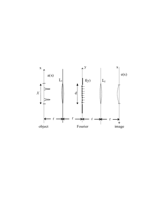
Figure 1: Optical scheme of one-dimensioned diffraction-limited optical imaging.

As mentioned above, to achieve superresolution one needs some a priori information about the object. In our case we know a priori that the object is confined within the area of size $X$ and is identically zero outside. The spatial Fourier transform of such an object is an entire analytical function. Therefore, knowing the part of the Fourier spectrum within the area $d$ of the pupil allows for an analytical continuation of the total spectrum and, therefore, for unlimited resolution. However, this analytical continuation is extremely sensitive to the noise in the diffracted image and, as will be illustrated below, is limited by the quantum fluctuations of light.

To simplify notations we shall use the dimensionless coordinates $s=2x/X$ in the object and the image planes and the dimensionless coordinate $\xi=2y/d$ in the pupil (Fourier) plane. Let the classical dimensionless complex amplitudes of the electromagnetic field in the object, Fourier, and the image planes be respectively $a(s)$, $f(\xi)$, and $e(s)$. The amplitudes $a(s)$ and $f(\xi)$ are related by the Fourier transform performed by the lens $L_{1}$,

$$f(\xi)=\sqrt{\frac{c}{2\pi}}\int_{-1}^{1}a(s)e^{ics\xi}ds,$$ (1)

where $c=\pi dX/(2\lambda f)$ is the space-bandwidth product of the imaging system.

The second lens $L_{2}$ performs the inverse Fourier transform and creates an image in the image plane. The object and the image complex amplitudes are related by an integral operator,

$$e(s)=\int_{-1}^{1}\frac{\sin[c(s-s^{\prime})]}{\pi(s-s^{\prime})}a(s^{\prime})ds^{\prime}.$$ (2)

The orthonormal eigenfunctions of this operator are given by

$$\varphi_{k}(s)=\frac{1}{\sqrt{\lambda_{k}}}\psi_{k}(s),\quad|s|\leq 1,$$ (3)

where $\psi_{k}(s)$ are the prolate spheroidal functions and $\lambda_{k}$ are the corresponding eigenvalues[4]. To achieve superresolution one can decompose the object field in the basis of the eigenfunctions $\varphi_{k}(s)$ as

$$a(s)=\sum_{k=0}^{\infty}a_{k}\varphi_{k}(s),\quad|s|\leq 1,$$ (4)

with the coefficients $a_{k}$ calculated by

$$a_{k}=\int_{-1}^{1}a(s)\varphi_{k}(s)ds.$$ (5)

Similar decomposition can be written in the image plane,

$$e(s)=\sum_{k=0}^{\infty}e_{k}\psi_{k}(s),\quad-\infty<s<\infty,$$ (6)

and in the Fourier plane,

$$f(\xi)=\sum_{k=0}^{\infty}f_{k}\varphi_{k}(\xi),\quad|\xi|\leq 1.$$ (7)

The coefficients $e_{k}$ are calculated as

$$e_{k}=\int_{-\infty}^{\infty}e(s)\psi_{k}(s)ds,$$ (8)

while the coefficients $f_{k}$ are given by

$$f_{k}=\int_{-1}^{1}f(\xi)\varphi_{k}(\xi)d\xi.$$ (9)

Using the properties of the prolate functions $\psi_{k}$ it can be shown that the coefficients $e_{k}$ and $f_{k}$ are expressed through $a_{k}$ as follows:

$$e_{k}=\sqrt{\lambda_{k}}a_{k},$$ (10)

$$f_{k}=i^{k}\sqrt{\lambda_{k}}a_{k}.$$ (11)

Therefore, detecting the image $e(s)$ in the image plane using, for example, a sensitive CCD camera, one can calculate the coefficients $e_{k}$ according to (8) and than reconstruct exactly the coefficients $a_{k}$ of the object using (10). Alternatively, one can set the CCD camera in the Fourier plane to detect $f(\xi),$ evaluate the coefficients $f_{k}$ according to (9) and reconstruct $a_{k}$ using (11). The first method could be called superresolving microscopy, while the second one superresolving Fourier-microscopy since one detects the Fourier spectrum. It should be noted that, since in both cases we need the complex field amplitudes and not the intensities, one should use the homodyne detection scheme with a local oscillator.

In our numerical simulations we have tried both detection schemes and have given preference to the Fourier-microscopy since it involves integration over the finite region of the pupil, while detecting the image $e(s)$ requires integration over an infinite area in the image plane. It turns out that due to oscillating behavior of the prolate functions $\psi_{k}(s)$ one needs to take unrealistically large area in the image plane to achieve significant superresolution.

For numerical simulations we have taken a simple object of two Gaussian peaks,

$$a(s)=\exp{\left(-\frac{(s-s_{0})^{2}}{2\sigma^{2}}\right)}+\exp{\left(-\frac{(s+s_{0})^{2}}{2\sigma^{2}}\right)},\quad|s|\leq 1,$$ (12)

of width $\sigma$ separated by distance $2s_{0}$. We choose $2s_{0}=1$ and $\sigma=0.1$, so that two peaks are well separated in the input object. The Rayleigh resolution distance $R=\pi X/(2c)$ in dimensionless coordinates is equal to $\pi/c$, where $c$ is the space-bandwidth product. In our simulations we work with $c=1$. In this situation for $2s_{0}<\pi$ we are beyond the Rayleigh limit. This is clearly seen in Fig. 2 where we have shown the input object and its image observed in the image plane.

Figure 2: Double-peak object $a(s)$ used in numerical simulations (a) and its image $e(s)$ (b).

Therefore, observing the image in Fig. 2b, it is impossible according to the Rayleigh criterion to resolve two Gaussian peaks in input object. However, applying the superresolution technique one can easily reconstruct the input object beyond the diffraction limit. We illustrate the result of such a reconstruction in Fig. 3. In this figure we show the exact Fourier spectrum of the input object, drown by a solid line, as a function of dimensionless coordinate $\xi$ in the Fourier plane. Only a part of this spectrum shown by a bold line, within the area of the pupil, $|\xi|\leq 1$, is transmitted to the image plane. This is a reason of very large diffraction spread in the image plane shown in Fig. 2b. Three dotted bold lines in Fig. 3 correspond to the Fourier spectrum of the reconstructed object using 2, 4, and 6 prolate functions. We can see that the reconstructed spectrum approaches the exact one for ever higher spatial frequencies $|\xi|$ as the number of prolate functions increases.

Figure 3: Spatial Fourier spectrum of the object from Fig. 2a (solid line), its part transmitted trough the pupil (bold solid line), and the spectra reconstructed with 2, 4, and 6 prolate functions (three dotted bold lines).

With 6 prolate functions two spectra are very close to each other for spatial frequencies $|\xi|\leq 8$. This corresponds to a superresolution factor of 8 over the Rayleigh limit.

Up to now we did not take into account the fluctuations in the detection of the Fourier components by a CCD camera in the Fourier plane. However, such fluctuations are always present in the detection scheme due to technical imperfections and the quantum nature of light. The quantum fluctuations of light set the ultimate limit of superresolution in optical imaging. The quantum theory of the optical imaging scheme in Fig. 1 was developed in Ref. [3]. Applying the same methods for the Fourier-microscopy, we can write the photon annihilation operators $\hat{a}(s)$ and $\hat{f}(\xi)$ in the object and the Fourier plane as

$$\hat{a}(s)=\sum_{k=0}^{\infty}\hat{a}_{k}\varphi_{k}(s)+\sum_{k=0}^{\infty}\hat{b}_{k}\chi_{k}(s),$$ (13)

$$\hat{f}(\xi)=\sum_{k=0}^{\infty}\hat{f}_{k}\varphi_{k}(\xi)+\sum_{k=0}^{\infty}\hat{g}_{k}\chi_{k}(\xi).$$ (14)

Here $\chi_{k}$ are the orthonormal basis functions in the region $|s|>1$ and $|\xi|>1$ introduced in Ref. [3], and $\hat{b}_{k}$ and $\hat{g}_{k}$ are the corresponding annihilation operators. It can be shown that the operator-valued Fourier coefficients $\hat{f}_{k}$ are given by

$$\hat{f}_{k}=i^{k}(\sqrt{\lambda_{k}}\hat{a}_{k}+\sqrt{1-\lambda_{k}}\hat{b}_{k}).$$ (15)

This relation is similar to the transformation performed by a beam-splitter with amplitude transmission coefficients $i^{k}\sqrt{\lambda_{k}}$ and reflection coefficients $i^{k}\sqrt{1-\lambda_{k}}$, and preserves the commutation relation of the annihilation and creation operators in the Fourier plane.

We can use Eq. (15) for calculation of the coefficients $\hat{a}_{k}^{(r)}$ in the reconstructed object as

$$\hat{a}_{k}^{(r)}=\frac{\hat{f}_{k}}{i^{k}\sqrt{\lambda_{k}}}=\hat{a}_{k}+\sqrt{\frac{1-\lambda_{k}}{\lambda_{k}}}\hat{b}_{k},$$ (16)

where the superscript $(r)$ indicates ”reconstructed”. As follows from Eq. (16), the reconstruction of the input object is no longer exact because of the second term in Eq. (16). This term contains the annihilation operators $\hat{b}_{k}$ responsible for the vacuum fluctuations of the electromagnetic field in the area outside the object. It is important to notice that these vacuum fluctuations prevent from reconstruction of the higher and higher coefficients $\hat{a}_{k}$ in the object because of the multiplicative factor $\sqrt{(1-\lambda_{k})/\lambda_{k}}$. Indeed, the eigenvalues $\lambda_{k}$ become rapidly very small after the index $k$ has attained some critical value. This leads to rapid ”amplification” of the vacuum fluctuations in the reconstructed object that limits the number of the reconstructed coefficients $\hat{a}_{k}$. Below we illustrate numerically the role of these quantum fluctuations in superresolution.

Figure 4: Reconstruction of the spatial Fourier spectrum of the object with light in a coherent state with mean photon number $\langle N\rangle=10^{12}$. Five dotted lines correspond to five random Gaussian realizations of the quantum fluctuations.

The relative value of quantum fluctuations depends on the signal-to-noise ratio in the input object which for the light in a coherent state is determined by the total mean number of photons passed through the object area during the observation time. For example, for a laser beam with $\lambda=1064$ nm and optical power of 1 mW, and observation time of 1 ms we obtain the mean photon number of $\langle N\rangle=5.3\cdot 10^{12}$.

In Fig. 4 we have shown the results of reconstruction of the spatial spectrum of the object from Fig. 2a when quantum fluctuations of a coherent state are taken into account. The solid line gives an exact spatial Fourier spectrum of the object and the solid bold line the part of the spectrum passed through the pupil as in Fig. 3. We use 6 prolate functions and the mean photon number in the input object is taken $\langle N\rangle=10^{12}$. The five dotted lines correspond to five random Gaussian realizations of the quantum fluctuations in the coherent state of $\hat{a}_{k}$ and the vacuum fluctuations of $\hat{b}_{k}$. The dotted bold line corresponds to the reconstructed spectrum by 6 prolate functions without noise (as in Fig. 2). One can observe that the role of quantum fluctuations becomes more and more important as one goes to the higher and higher spatial frequencies where the random realizations of the Fourier spectra deviate more and more from the mean value given by the dotted bold line.

In Fig. 5 we have increased the total mean value of photons to $\langle N\rangle=10^{13}$. This corresponds to an increased signal-to-noise ratio in the input object and should allow for better superresolution. This is illustrated in Fig. 5 where we can reconstruct higher spatial frequencies in the Fourier spectrum as compared to Fig. 4.

Figure 5: Same as Fig. 4 but with $\langle N\rangle=10^{13}$.

The same result can be achieved by using multimode squeezed light instead of increasing the power of the source illuminating the object. This is illustrated in Fig. 6 where we have used $\langle N\rangle=10^{12}$ as in the Fig. 4, but considered the light in a multimode squeezed state with the squeezing parameter $e^{r}=10$ instead of the coherent state. As the result the fluctuations in the higher spatial frequencies are decreased that gives better superresolution.

Figure 6: Reconstruction of the spatial Fourier spectrum of the object with light in multimode squeezed state with mean photon number $\langle N\rangle=10^{12}$ and the squeezing parameter $e^{r}=10$.

In conclusion, we have numerically investigated the role of quantum fluctuations in reconstruction of spatial spectra of optical objects. We have demonstrated that when quantum fluctuations are not taken into account one can achieve superresolution of about factor 10 over the Rayleigh limit. We have confirmed that the limit of superresolution is set by quantum fluctuations and depends on the signal-to-noise ratio in the input object. For a given signal-to-noise ratio one can further improve superresolution by using multimode squeezed light.

This work was supported by the Network QUANTIM [5] (IST-200-26019) of the European Union.

References

- [1] M. I. Kolobov, Rev. Mod. Phys. 71, 1539 (1999).
- [2] ”Quantum fluctuations and coherence in optical and atomic structures”, special issue of the Eur. Phys. J. D 22 (2003).
- [3] M. I. Kolobov and C. Fabre, \Journal\PRL8537892000.
- [4] D. Slepian and H. O. Pollak, Bell System Techn. J. 40, 43 (1961).
- [5] http://sucima.dipscfm.uninsubria.it/quantim/