Entanglement as a signature of quantum chaos

Abstract

We explore the dynamics of entanglement in classically chaotic systems by considering a multiqubit system that behaves collectively as a spin system obeying the dynamics of the quantum kicked top. In the classical limit, the kicked top exhibits both regular and chaotic dynamics depending on the strength of the chaoticity parameter $\kappa$ in the Hamiltonian. We show that the entanglement of the multiqubit system, considered for both bipartite and pairwise entanglement, yields a signature of quantum chaos. Whereas bipartite entanglement is enhanced in the chaotic region, pairwise entanglement is suppressed. Furthermore, we define a time-averaged entangling power and show that this entangling power changes markedly as $\kappa$ moves the system from being predominantly regular to being predominantly chaotic, thus sharply identifying the edge of chaos. When this entangling power is averaged over initial states, it yields a signature of global chaos. The qualitative behavior of this global entangling power is similar to that of the classical Lyapunov exponent.

I Introduction

Quantization of classical chaotic systems has long been of interest because of the challenges in identifying quantum signatures of systems that, in a classical limit, exhibit chaotic behavior. Various signatures have been identified, such as the spectral properties of the generating Hamiltonian HaakeBook , phase space scarring Scar , hypersensitivity to perturbation Hyper , and fidelity decay Fidelity , which indicate an underlying chaotic presence in the quantum dynamics. Here, we investigate the issue of quantum signatures from the perspective of entanglement: as entanglement is at the heart of quantum mechanics and a crucial resource for quantum information processing Nie00 ; Bennett , the entanglement inherent in quantum chaotic systems could provide a valuable approach to studying decoherence and quantum chaos Zurek93 ; Fur98 ; Mil99 ; Lak01 ; Ban02 ; Fuj03 . Furthermore, quantum chaos could be seen as an engine for generating entanglement; indeed quantum chaos could lurk in quantum information processing Bettelli03 ; SC2003 ; She00 as a deleterious or perhaps even as an advantageous effect. We study entanglement by considering a finite multipartite system, whose collective dynamics obey chaotic Hamiltonian dynamics in the classical limit.

Previous studies of entanglement in chaotic systems  Zurek93 ; Fur98 ; Mil99 ; Lak01 ; Ban02 ; Fuj03 ; Bettelli03 ; SC2003 have explored bipartite entanglement in pure states, entanglement of qubits in a multiqubit system and average entanglement or entangling power. In this study we explore these different types of entanglement in a single simple system, namely the quantum kicked top (QKT) Haa86 ; Haa87 ; Fra85 ; Schack94 ; BarryChaos . This enables us to compare the degree to which these different types of entanglement display signatures of chaos.

An advantage of the dynamics of the QKT is that it obeys a spin algebra symmetry. This spin system can thus be regarded as a composite of distinct spin-half particles thereby admitting a multiqubit interpretation. Our system thus allows us to study and compare pairwise entanglement between two qubits as well as bipartite entanglement between the two qubits and the rest of the qubits. The Hilbert space for the QKT is finite and the Poincaré section of the phase space compact, allowing analyses of quantum and classical dynamics uncomplicated by truncation issues. The QKT is well studied and understood thereby simplifying the analysis of the role of entanglement in the system. Finally, the QKT possesses a parity symmetry that allows coherent quantum tunnelling to occur for states localized at classical fixed points BarryChaos .

The Hamiltonian evolution may increase the entanglement of the multipartite system, initiated in a collective spin coherent state SCSS . For this analysis it suffices to employ two entanglement measures. For bipartite entanglement, where the multipartite system is divided into two subsystems, entropy of a subsystem is used to quantify the degree of entanglement between the two subsystems. Pairwise entanglement, on the other hand, considers the degree of entanglement between two qubits traced over all remaining qubits and is quantified by the concurrence wootters1 ; wootters2 .

We present general results for both bipartite and pairwise entanglement in the multipartite QKT and demonstrate that these entanglement measures reveal strong signatures of the classical chaos features corresponding to the onset of chaos and to the edge of chaos Edge , which is the boundary between regular and chaotic regimes in the classical phase space. We have studied the behavior of the linear entropy and the concurrence for specific initial states as well as the dynamics of these quantities when averaged over all initial states. We show that the linear entropy increases more rapidly for an initial state centered in a chaotic region of the classical phase space than one centered on a fixed point. This agrees with the behavior of the linear entropy observed in other chaotic systems, supporting the conjecture that classical chaos can enhance bipartite entanglement Zurek93 ; Fur98 . Furthermore, we show that the pairwise entanglement as measured by the concurrence also reveals a dramatic change for a spin coherent state whose mean traverses the edge of chaos on its transit through chaotic and regular regions of the phase space. Contrary to the linear entropy, the concurrence rapidly decreases for an initial state located in the chaotic region.

While the linear entropy and concurrence can reveal the local chaotic and regular structures in phase space, the entangling power, which is the averaged bipartite or pairwise entanglement, can be used to identify the edge of chaos and quantify the onset of global chaos, much like the classical Lyapunov exponent. We show that the entangling power greatly increases as the chaoticity parameter $\kappa$ is increased, and the corresponding classical kicked top makes the transition from predominantly regular to predominantly chaotic behavior. In particular, the behavior of the average linear entropy is qualitatively similar to that of the classical Lyapunov exponent, thus revealing a signature of a global feature of the classical chaos.

The paper is organized as follows. In Sec. II, we introduce the QKT and its classical dynamics, and introduce bipartite and pairwise entanglement measures. In Sec. III, we study in detail dynamical evolutions of bipartite and pairwise entanglement, and examine the edge of quantum chaos, the onset of quantum chaos via the entangling power. We conclude in Sec. IV.

II Background

II.1 Quantum kicked top

The QKT is described by the Hamiltonian Haa86 ; Haa87 ; Fra85

$$H=\frac{\kappa}{2j\tau}J_{z}^{2}+pJ_{y}\sum_{n=-\infty}^{\infty}\delta(t-n\tau),$$ (1)

where $J_{\alpha}~{}(\alpha\in\{x,y,z\})$ are spin operators and states are restricted to irrep $j$ for which $J^{2}=j(j+1)$. $\tau$ is the duration between periodic kicks, $p$ is the strength of each kick (which is manifested as a turn by angle $p$), and $\kappa$ is the strength of the twist. The Hamiltonian is an alternative sequence of twists ($J_{z}^{2}$ term) and turns ($J_{y}$ term). The QKT describes a spin system, which can be comprised of multiple systems of lower spins. For $\{\sigma_{i\alpha}\}$ the Pauli operators for the $i^{\text{th}}$ qubit, a collective spin operator, satisfying the usual su(2) algebra, is given by

$$J_{\alpha}=\sum_{i=1}^{N}\frac{\sigma_{i\alpha}}{2}.$$ (2)

An example of using multiple qubits to simulate the QKT has been presented for trapped ions Milburn99 .

A standard dynamical description of the QKT is via the Floquet operator

$$F=\exp\left(\text{-i}\frac{\kappa}{2j\tau}J_{z}^{2}\right)\exp\left(\text{-i}pJ_{y}\right),$$ (3)

where the energy is rescaled so that $\tau=1$, and $p=\pi/2$ are henceforth assumed. The orthogonal eigenstates of $F$, denoted by $\{|\Phi_{m}\rangle:-j\leq m\leq j\}$, which satisfy

$$F|\Phi_{m}\rangle=\exp(\text{i}\Phi_{m})|\Phi_{m}\rangle,$$ (4)

provide a convenient basis for stroboscopic evolution. An arbitrary state $|\Psi(0)\rangle$ evolves to

$$|\Psi(n)\rangle=F^{n}|\Psi(0)\rangle=\sum_{m=-j}^{j}\Psi_{m}(0)\exp(\text{i}n\Phi_{m})|\Phi_{m}\rangle.$$ (5)

with $\Psi_{m}(0)=\langle\Phi_{m}|\Psi(0)\rangle$.

The QKT Haa86 ; Haa87 is chaotic in the classical limit. For integrable systems, it is well known from semi-classical theory that the classical actions can be associated with corresponding regular eigenstates of the quantum system with a well defined quantum number. This correspondence breaks down in chaotic systems E1917 . In quasi-integrable systems with a mixed classical phase space of regular and chaotic regions, some of the eigenstates can still be associated with local actions in the regular regions with corresponding discrete eigenenergies. The remaining eigenstates result in an irregular energy spectrum corresponding to the chaotic region P1973 . We show here that this underlying regular and chaotic energy spectrum of the Floquet eigenstates of the QKT is reflected in the dynamics of the entanglement, depending on whether the initial state is in the regular or chaotic region of the classical phase space.

The classical limit of the QKT is obtained by expressing $X=\langle J_{x}/j\rangle$ and similar for $Y$ and $Z$ and factorizing all moments such as $\langle J_{x}J_{y}/j^{2}\rangle=XY$ to products of first-order moments. Then the classical equations of motion, obtained from the Heisenberg operator equations of motion and applying the factorization rule above, are given by Haa87

$$X^{\prime} = Z\cos(\kappa X)+Y\sin(\kappa X),$$

$$Y^{\prime} = -Z\sin(\kappa X)+Y\cos(\kappa X),$$ (6)

$$Z^{\prime} = -X$$

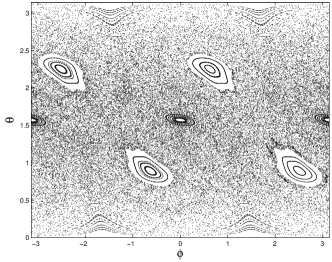
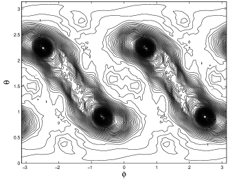
The stroboscopic evolution described by Eq.(6) can be represented in a phase space given by a sphere $\mathcal{S}^{2}$ of unit radius. The classical, normalized angular momentum variables $(X,Y,Z)$ can be parametrized in polar coordinates as $(X,Y,Z)=(\sin\theta\cos\phi,\sin\theta\sin\phi,\cos\theta),$ where $\theta$ and $\phi$ are the polar and azimuthal angles, respectively. Thus the mapping domain is essentially two-dimensional.

The stroboscopic dynamics of the classical map is shown in Fig. 1. In the plot, we choose the chaoticity parameter $\kappa=3$ which yields a mixture of regular and chaotic areas of significant size. Elliptic fixed points surrounded by the chaotic sea are evident. Two such elliptic fixed points have coordinates $(\theta,\phi)=(2.25,-2.51)$ and $(\theta,\phi)=(2.25,0.63).$ As we will see, this phase space structure of the classical kicked top determines behavior of quantum entanglement in the QKT.

Figure 1: The stroboscopic phase space dynamics of the classical kicked top for $\kappa=3.$ Three hundred stroboscopic trajectories are plotted, each for a duration of 300 kicks.

II.2 Entanglement measures

Pure-state bipartite entanglement has been calculated in previous studies that explore connections between quantum entanglement and underlying classical chaos Fur98 ; Mil99 ; Lak01 ; Ban02 ; Fuj03 . Quite recently, Bettelli and Shepelyansky Bettelli03 studied the behavior of the concurrence in a system exhibiting quantum chaos, and found that the underlying classical chaos leads to exponential decrease of the concurrence down to some residual values. This result shows that the concurrence is very sensitive to the onset of chaos, and understanding entanglement of these systems may help to control quantum chaos and suppress its negative effects in quantum information processing.

We consider bipartite entanglement between a pair of qubits selected from a symmetric multi-qubit state and the rest of the system, as well as pairwise entanglement between the two qubits. Once we obtain the two-qubit reduced density matrix, the entanglement can be readily calculated. By expressing the reduced density matrix $\rho_{12}$ for qubit 1 and 2 in terms of the expectation values of the collective operators, all elements of $\rho_{12}$ are conveniently obtained WangKlaus .

Our system governed by the QKT Hamiltonian is a composite system, and remains in a pure state at all times if we initially choose a pure state. For pure states, bipartite entanglement is well-defined and can be quantified by entropies of either subsystem. For convenience, we adopt the linear entropy as the entanglement measure, which is defined as

$$E=1-\text{Tr}_{1}(\rho_{1}^{2}),$$ (7)

where $\rho_{1}$ is the reduced density matrix for the first subsystem. The maximum linear entropy for a pure state of a bipartite $d_{1}\times d_{2}$ system, is given by $1-1/\min(d_{1},d_{2})$. While we may choose other entropies such as the von Neumann entropy as our entanglement measure, the qualitative results are in general independent of choice of entropies for pure states. Moreover, the linear entropy and the von Neumann entropy are two limiting cases of the Rényi entropy Renyi , they are thus interrelated and one can be used to estimate the other Entropy1 ; Entropy2 .

Given our $N$-qubit system, we consider another type of entanglement, the pairwise entanglement, i.e., the entanglement between a pair of qubits. When $N\geq 3$, the pair of qubits can be in a mixed state. Entanglement for a mixed state $\rho_{12}$ is quantified by the entanglement of formation. Specifically, for a pair of qubits, entanglement is equivalent to the non-positivity of the partially transposed density matrix peres . Alternatively, one can use the concurrence wootters1 ; wootters2 to quantify the pairwise entanglement. The concurrence is defined as

$$\mathcal{C}=\max\left\{0,\lambda_{1}-\lambda_{2}-\lambda_{3}-\lambda_{4}\right\},$$ (8)

with the quantities $\lambda_{i}$ being the square roots of the eigenvalues in descending order of the matrix product $\rho_{12}(\sigma_{1y}\otimes\sigma_{2y})\rho_{12}^{\ast}(\sigma_{1y}\otimes\sigma_{2y}).$ $\rho_{12}^{\ast}$ denotes the complex conjugate of $\rho_{12}$. The value of the concurrence ranges from zero for an unentangled state to unity for a maximally entangled state.

III Entanglement and quantum chaos

We present here our studies of the entanglement dynamics of our $N$-qubit system governed by the QKT (1), with the relevant angular momentum operators $J_{\alpha}$ given by the collective operators. If we choose the initial pure state to be symmetric under exchange of any qubits, then the state vector at any later time is also symmetric. Thus, we can describe the state of the $N$-qubit system in terms of the orthonormal basis $\{|j,m\rangle;(m=-j,-j+1,...,j)\}$ with $j=N/2$. The states $\{|j,m\rangle\}$ are the usual symmetric Dicke states Dic54 . State $|j,-j\rangle$ is not entangled, whereas state $|j,-j+1\rangle$, the so-called W state Dur00 ; Wang1 , is pairwise entangled with concurrence ${\cal C}=2/N$.

To connect the quantum and classical dynamics of the kicked top, we choose the initial state to be the spin coherent state (SCS) $\{|\theta,\phi\rangle=R(\theta,\phi)|j,j\rangle;-\pi\leq\phi\leq\pi,0\leq\theta\leq\pi\}$, with SCSS

$$R(\theta,\phi)=\exp\{\text{i}\theta[J_{x}\sin\phi-J_{y}\cos\phi]\}.$$ (9)

Mean of $\mathbf{J}/j$ is

$$\langle\theta,\phi|\mathbf{J}/j|\theta,\phi\rangle=(\sin\theta\cos\phi,\sin\theta\sin\phi,\cos\theta).$$ (10)

The initial SCS can be rewritten as a multi-qubit product state, and thus exhibits no entanglement (zero linear entropy and concurrence).

III.1 Dynamics of entanglement

We start by exploring the dynamics of entanglement for initial states with a mean value in four different regions of the phase space, specifically a fixed point, an integrable (or KAM) region, a chaotic region, and the border between the integrable and the chaotic region known as ‘the edge of chaos’ Edge . We are also interested in the behavior as the chaoticity parameter $\kappa$ is varied. We start with the choice $\kappa=3$, which exhibits large integrable and large chaotic regions, and we select four states localized in the four regions mentioned earlier.

For convenience we fix $\theta=2.25$ and vary $\phi$: this ‘line of latitude’ on $\mathcal{S}^{2}$ includes all four regions we are exploring. An elliptic fixed point arises at $\phi=0.63$, a point in the regular region occurs at $\phi=0.90$, one edge of chaos can be seen at $\phi=1.05$, and a point well in the chaotic sea is located at $\phi=2.00$. The states with means at each of these $(\theta,\phi)$ points in the phase space are chosen to be SCSs. These states are minimum uncertainty states and are well localized around the four chosen points in phase space.

Figure 2: Dynamical evolution of the linear entropy for initial SCS $|\theta=2.25,\phi$ for $\kappa=3$ and $N=50$.

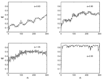
We numerically compute bipartite entanglement between two qubits and the other $N-2$ qubits, and display the numierical results in Fig. 2 as linear entropy versus time increasing parameter $n$. We observe that the entanglement is enhanced for the initial state centered in the chaotic region after a short time. Initially, the linear entropy is zero, and as the dynamics evolve, the entropy increases slowly when the wave packet is centered in the regular region, whereas it exhibits a rapid rise when centered in the chaotic region. The curve with $\phi=1.05$ displays the intermediate behavior. Furthermore, the entanglement for the state initially with mean at a fixed point displays a periodic modulation that is absent in the evolution of the entanglement for the state initiated in the chaotic region. This periodic modulation is an indicator of the underlying regular classical dynamics and corresponding regular energy spectrum of the Floquet eigenstates P1973 .

Figure 3: Dynamical evolution of the concurrence. The parameters are the same as those of Fig. 2.

Figure 4: Long time behavior of the concurrence for the regular case ($\theta=2.25,\phi=0.63$). The other parameters are the same as those of Fig. 2.

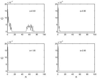
Figure 3 shows the dynamical behavior of the concurrence. Just as in the linear entropy case, we see a rapid change in the concurrence for a state initially centered in the chaotic sea. However, our numerical results suggest that the initial state centered in the fixed point will lead to large pairwise entanglement production, which is opposite to the case of the bipartite pure-state entanglement production, in which the classical chaos enhances the production of bipartite entanglement. Of particular interest are the collapses and revivals in the evolution of the concurrence for a state centered on the fixed point. Figure 3 (left-up one) shows a revival at $n=52$. Additional revivals occur at $n=113$, $n=183$ and so on. For the chaotic case, we cannot observe the revival phenomenon. This quasiperiodic behavior in the regular region indicates that the SCS in the regular region has a finite support over the basis set of regular Floquet eigenstates.

In Fig. 4 we plot the long-time behaviors of the concurrence for the regular case, and observe multiple collapse and revivals. At long times the revivals become sparse, and finally the concurrence reduces to zero. We see that the concurrence is very sensitive to quantum chaos, which is consistent with the observations of Bettelli and Shepelyansky Bettelli03 in their studies of concurrence between qubits during the operation of an efficient multiqubit quantum algorithm. However, unlike their system in which the concurrence reached a finite residual value, in our QKT model, the concurrence disappears at very long times; the difference arises because we assumes symmetrised multi-qubit states, whereas Bettelli and Shepelyansky allow this symmetry to be broken.

III.2 Edge of quantum chaos

The edge of chaos Edge is an important issue in the study of quantum chaos. In classical chaos, the edge of chaos is a fractal boundary separating the regular and chaotic regions. However, this fine-grained fractal structure does not translate well into the quantum domain. Recently, it was found that the edge of chaos is characterized by a power law decrease in the overlap between a state evolved under chaotic dynamics and the same state evolved under a slightly perturbed dynamics Edge . Here, we study the edge of quantum chaos from the perspective of entangling powers, which are defined to be either the maximal or the mean entanglement that the evolution operator can generate over all initial states P ; Paolo . Alternatively, given a fixed initial state, we may ask what is the maximal and the mean entanglement that the operator can generate over all time. In general state-averaging and time-averaging are inequivalent and so the two methods yield different results.

In strongly chaotic systems, the two definitions converge due to nearly ergodic dynamics. In this study, we explore both the entanglement averaged over all time as well as the entanglement averaged over initial states. We begin our analysis with the average over time. In practice, for numerical purposes we consider a finite time domain. We define time-averaged entanglement power as the average linear entropy or average concurrence over a time interval $T$ (which should be much longer than other time scales) as follows:

$$E_{T}=\frac{1}{T}\int_{0}^{T}\text{d}t~{}E(t),\,{\cal C}_{T}=\frac{1}{T}\int_{0}^{T}\text{d}t~{}{\cal C}(t).$$ (11)

For local unitary operations, the above quantities are necessarily zero.

Figure 5: Mean linear entropy and mean concurrence against azimuthal angle $\phi$. The mean linear entropy is plotted for $N=20$ (solid line), $N=50$ (dashed line), and $N=100$ (dotted line); the mean concurrence is plotted for $N=100$ (solid line), $N=200$ (dashed line), and $N=300$ (dotted line). Parameters $\theta$ and $\kappa$ are set to $\theta=2.25$ and $\kappa=3$. The time average is over 200 steps, and the subplots below are partly enlarged versions of above ones.

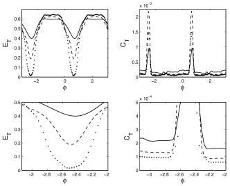
We fix the polar angle $\theta=2.25$ of the SCS as before, and vary the azimuthal angle $\phi$ from $-\pi$ to $\pi$. The center of the SCS wave packet thus commences in the chaotic region and passes through two regular islands. Figure 5 displays the time-averaged mean linear entropy $E_{T}$and mean concurrence $C_{T}$ as a function of the azimuthal angle $\phi$. When the azimuthal angle goes from $-\pi$ to the first regular region, the linear entropy decreases until it reaches a minimum which approximately corresponds to the fixed point $(\theta,\phi)=(2.25,-2.51)$. Subsequently the mean entropy increases to a flat larger area corresponding to the chaotic region.

In contrast to the behavior of the mean linear entropy, the mean concurrence reaches a maximum approximately at the fixed point. When $\phi$ increases from $-\pi$, the mean concurrence first decreases slowly, and then exhibits an abrupt increase to a maximal value. Thos turning point sharply displays the edge of chaos. Another turning point is obvious from the figure.

We also observe that the larger the number of qubits, the wider the regular region. In the large $N$ limit, the regular region will coincide with that of corresponding classical chaos of Fig. 1.

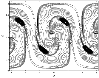
We further calculate the mean linear entropy and the mean concurrence as a function of $\theta$ and $\phi$. The contour plots are shown in Figs. 4 and 5. Comparing Figs. 1 and 4, we observe that these two figures closely match each other. Specifically, the four islands of Fig. 4 are evident, reflecting the four stable islands in the classical phase space. Comparing Figs. 1 and 5, the four stable islands of Fig. 1 closely match those of Fig. 5. Thus, we have a good classical-quantum correspondence.

Figure 6: Contour plot of mean linear entropy against $\phi$ and $\theta$. The mean is over 200 kicks and other parameters are the same as those in Fig. 2.

Figure 7: Contour plot of mean concurrence against $\phi$ and $\theta$. The average is over 200 kicks and other parameters are the same as those in Fig. 2.

III.3 Onset of Chaos

Figure 8: Entangling power $e_{T}$ (square line), $c_{T}$ (diamond line), and the Lyapunov exponent $\lambda$ (circle line)agaist $\kappa$. The plot of Lyapunov exponent corresponds to fig. 1 of Ref. LY . The parameter $N=36$ and time average is over 50 kicks.

In the previous section, the time-averaged entanglement revealed clearly whether the initial state was in the regular or chaotic region. Here, we are concerned with global properties of a chaotic system. For classical systems, the onset of global chaos can be quantified by calculating the global Lyapunov exponent. Here we define the following entangling power to quantify the onset of global quantum chaos:

$$e_{T}=\frac{1}{T}\int\text{d}\mu\int_{0}^{T}\text{d}t~{}E(t,\theta,\phi),$$

$${c}_{T}=\frac{1}{T}\int\text{d}\mu\int_{0}^{T}\text{d}t~{}{\cal C}(t,\theta,\phi),$$ (12)

where $\text{d}\mu=\text{d}\mu(\theta,\phi)$ is the Haar measure. Like the global classical Lyapunov exponent, this state-averaged entangling power characterizes global properties of the QKT. The entangling power characterizes the entangling capability of the $\kappa$-dependent Floquet operator.

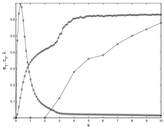
Figure 8 shows the entangling powers and the Lyapunov exponent versus parameter $\kappa$. We observe that when $\kappa=\kappa_{0}\approx 2.4$, the entangling power $e_{T}$ exhibits a rapid increase and saturates beyond $\kappa=\kappa_{1}\approx 5$. The rapid increase of the entangling power signifies the onset of quantum chaos, and the saturation implies that global chaos has occurred. Between $\kappa_{0}$ and $\kappa_{1}$, when there are still regions of regular islands in the chaotic phase space, a mixture of regular and chaotic behavior is expected. In contract to $e_{T}$, $c_{T}$ becomes very small for $\kappa>\kappa_{0}$, which is also an indicator of onset of quantum chaos. Note that $c_{T}$ has a peak which results from the competition between the entangling power of the QKT Floquet operator and the inherent chaos. On one hand, increasing $\kappa$ will enhance the entangling power, and on the other hand, the inherent quantum chaos suppresses the pairwise entangling power, thus leading to the peak. For $e_{T}$, increase of $\kappa$ and the quantum chaos both enhance the linear entropy, and thus no competition exists and no peak appears.

IV Conclusions

We have investigated a multi-qubit system whose collective Hamiltonian dynamics are chaotic in the classical limit. We studied the particular example of the quantum kicked top, which is a well-studied example of quantum chaos with the advantages of having a finite-dimensional Hilbert space (thereby obviating the need for truncation that arises in infinite-dimensional Hilbert spaces) and of involving only spin operators of no more than quadratic order.

Although the collective dynamics are well understood, the underlying entanglement of the qubits that collectively make up the quantum kicked top is only just beginning to be understood. Here we have developed methods for studying the quantum kicked top, and these methods are applicable to more general systems. We have identified bipartite and pairwise entanglement as two quite distinct measures to determine the entanglement in the system, and we have related the dynamics of these measures of entanglement to chaotic features of the quantum kicked top in the classical limit; as examples, we have connected the features of the entanglement evolution to local properties such as whether the state is supported predominantly in the regular or chaotic region and also to global properties such as showing that entangling power averaged over states grows similarly to the global Lyapunov exponent growth for the classical chaotic system.

We have assumed symmetric multi-qubit states throughout, and the entanglement properties studied here reflect this assumption. If the symmetrization condition is broken, different dynamics can be expected. For example, Bettelli and Shepelyanski Bettelli03 show a concurrence that reaches a residual steady-state value. They explain this non-zero residue as being a result of symmetry breaking in their system. In contrast, our system exhibits a decay of concurrence to zero. The assumption of symmetric states implies indistinguishability of the qubits. Thus even though entanglement may exist in the system, it may not be accessible as a useful tool for quantum information processing due to inherent inability to distinguish between the qubits. An alternative measure of entanglement could be an operational measure that takes into account physical restrictions on accessibility of the entanglement due to symmetries of the system WV2003 .

In summary, our work highlights the connection between entanglement of a multi-qubit state whose collective dynamics is chaotic in the classical limit and introduces valuable methods and measures for studying this entanglement. It would be worthwhile to investigate other quantum chaotic systems using concepts of time-averaging and global entangling power. Furthermore, it would interesting to define and compare systems in which the symmetrization results hold to systems where this symmetrization condition is broken.