PARTIALITY IN PHYSICS

Abstract

We revisit the standard axioms of domain theory with emphasis on their relation to the concept of partiality, explain how this idea arises naturally in probability theory and quantum mechanics, and then search for a mathematical setting capable of providing a satisfactory unification of the two.

1 Introduction

Dana Scott[13] introduced domains more than thirty years ago as an appropriate mathematical universe for the semantics of programming languages. A domain is a partially ordered set with intrinsic notions of completeness and approximation. Recently[6], the authors have proven the existence of a natural domain theoretic structure in probability theory and quantum mechanics. The way to understand this structure is with the aid of the concept partiality.

To illustrate, in the domain $(\mathcal{P}\omega,\subseteq)$, the powerset of the natural numbers ordered by inclusion, a finite set will be partial, while the set $\omega$ will be total. In the domain $(\Sigma^{\infty},\sqsubseteq)$, the domain of bit streams with the prefix order, a finite string is partial, the infinite strings are total. In the domain $({\mathbf{I}}\,\!{\mathbb{R}},\sqsubseteq)$, the collection of compact intervals $[a,b]$ of the real line ordered by reverse inclusion, an interval like $[p,q]$ with $p<q$ rational is partial, while a one point interval $[x]$ representing a real number is total. In the domain $(\Omega^{n},\sqsubseteq)$, the $n$ dimensional mixed states in the spectral order (to be defined later), a pure state is total, while mixed states which are not pure are partial. In all the cases above, total elements coincide with elements which are maximal in the given order.

As we can see, the partiality idea arises naturally in both computer science and physics. The idea is important in computer science. We will review results herein which show that by reasoning about density operators as partial and total objects, one can derive the classical and quantum logics of Birkhoff and von Neumann as special order theoretic subsets. Because of this, we conclude that partiality is also an important idea in physics. Given that the idea is important, the main question asked in this paper is “What is an appropriate mathematical setting for discussing partiality?”

First we review the traditional axioms for domains, which succeed at capturing the notion partiality for objects like sets, strings and intervals. Then we consider the Bayesian and spectral orders on classical and quantum states, which are ‘domains’ that possess the same notion of completeness as do classical domains, but differ in that they offer a new notion of approximation. We then enumerate much of what we know about the order theoretic structure of these two new domains in the hope that it will point the way for an inspired reader to discover a proper generalization of classical domains that will have desirable properties useful to both physicists and computer scientists.

2 Domain theory

As we mentioned in the introduction, a domain $(D,\sqsubseteq)$ is a partially ordered set with notions of completeness and approximation. The completeness can be used for example to prove fixed point theorems, which themselves might be used to provide a semantics for recursion, or establish the existence of solutions to ordinary differential equations. Explaining approximation is more difficult.

The order on a domain can be used to define many topologies, some of which can be used to recover notions of limit that we are familiar with from analysis. One use for approximation – which itself is a relation $\ll$ contained in $\sqsubseteq$ – is that it can clarify these topologies for us, helping us to connect them to more familiar ideas. A more subtle use for approximation is in formalizing the notion partiality. To give a simple example, an object $x\in\mathcal{P}\omega$ approximates something – formally, there is $y$ with $x\ll y$ – if and only if $x$ is finite.

2.1 Order

A poset is a partially ordered set, i.e., a set together with a reflexive, antisymmetric and transitive relation.

Definition 2.1

Let $(P,\sqsubseteq)$ be a partially ordered set. A nonempty subset $S\subseteq P$ is directed if $(\forall x,y\in S)(\exists z\in S)\>x,y\sqsubseteq z$. The supremum of $S\subseteq P$ is the least of all its upper bounds provided it exists. This is written $\bigsqcup S$.

Definition 2.2

For a subset $X$ of a poset $P$, set

$$\uparrow\!\!X:=\{y\in P:(\exists x\in X)\,x\sqsubseteq y\}\ \ \&\ \downarrow\!\!X:=\{y\in P:(\exists x\in X)\,y\sqsubseteq x\}.$$

We write $\uparrow\!x=\,\uparrow\!\{x\}$ and $\downarrow\!x=\,\downarrow\!\{x\}$ for elements $x\in X$.

A partial order allows for the derivation of several intrinsically defined topologies.

Definition 2.3

A subset $U$ of a poset $P$ is Scott open if

1. $U$ is an upper set: $x\in U\ \&\ x\sqsubseteq y\Rightarrow y\in U$, and

2. $U$ is inaccessible by directed suprema: For every directed $S\subseteq P$ with a supremum,

   $$\bigsqcup S\in U\Rightarrow S\cap U\neq\emptyset.$$

The collection of all Scott open sets on $P$ is called the Scott topology.

Unless explicitly stated otherwise, all topological statements about posets are made with respect to the Scott topology.

Proposition 2.4

A function $f:P\rightarrow Q$ between posets is continuous iff

1. f is monotone: $x\sqsubseteq y\Rightarrow f(x)\sqsubseteq f(y).$

2. f preserves directed suprema: For every directed $S\subseteq P$ with a supremum, its image $f(S)$ has a supremum, and

   $$f(\bigsqcup S)=\bigsqcup f(S).$$

The completeness of domains comes from the fact that directed sets have suprema:

Definition 2.5

A dcpo is a poset in which every directed subset has a supremum. The least element in a poset, when it exists, is the unique element $\bot$ with $\bot\sqsubseteq x$ for all $x$.

Here is the most well-known fixed point theorem in domain theory.

Theorem 2.6

Let $f:D\rightarrow D$ be a Scott continuous map on a dcpo with a least element. Then

$$\mathrm{fix}(f):=\bigsqcup_{n\geq 0}f^{n}(\bot)$$

is the least fixed point of $f$.

The set of maximal elements in a dcpo $D$ is

$$\max(D):=\{x\in D:\ \uparrow\!\!x=\{x\}\}.$$

Each element in a dcpo has a maximal element above it.

Example 2.7

Let $X$ be a compact Hausdorff space. Its upper space

$${\mathbf{U}}\,\!{\mathit{X}}=\{\emptyset\neq K\subseteq X:K\mbox{ is compact}\}$$

ordered under reverse inclusion

$$A\sqsubseteq B\Leftrightarrow B\subseteq A$$

is a dcpo: For directed $S\subseteq{\mathbf{U}}\,\!{\mathit{X}}$, $\bigsqcup S=\bigcap S.$ A continuous map $f:X\rightarrow X$ induces a Scott continuous map

$$\bar{f}:{\mathbf{U}}\,\!{\mathit{X}}\rightarrow{\mathbf{U}}\,\!{\mathit{X}}::K\mapsto f(K)$$

and since $\bot=X\in{\mathbf{U}}\,\!{\mathit{X}}$, the fixed point theorem guarantees that

$$\mathrm{fix}(\bar{f}):=\bigcap f^{n}(X)$$

is the least fixed point of $\bar{f}$. That is, $f$ has a unique largest invariant set $K=f(K)$. If $f$ were a contraction, then we would have $K=\{x^{*}\}$, where $x^{*}$ is the unique fixed point of $f$.

It is interesting here that the space $X$ can be recovered from ${\mathbf{U}}\,\!{\mathit{X}}$ in a purely order theoretic manner: It can be shown that

$$X\simeq\max({\mathbf{U}}\,\!{\mathit{X}})=\{\{x\}:x\in X\}$$

where $\max({\mathbf{U}}\,\!{\mathit{X}})$ carries the relative Scott topology it inherits as a subset of ${\mathbf{U}}\,\!{\mathit{X}}.$ Several constructions of this type are known, especially for Hilbert spaces. This illustrates one way that an order can implicitly describe a topology.

2.2 Approximation and continuity

Domains are posets that carry intrinsic notions of approximation and completeness.

Definition 2.8

For elements $x,y$ of a poset, write $x\ll y$ iff for all directed sets $S$ with a supremum,

$$y\sqsubseteq\bigsqcup S\Rightarrow(\exists s\in S)\>x\sqsubseteq s.$$

We set $\mathord{\mbox{\makebox[0.0pt][l]{\raisebox{-1.72218pt}{$\downarrow$}}$\downarrow$}}x=\{a\in D:a\ll x\}$ and $\mathord{\mbox{\makebox[0.0pt][l]{\raisebox{1.72218pt}{$\uparrow$}}$\uparrow$}}x=\{a\in D:x\ll a\}$.

For the symbol “$\ll$,” read “approximates.”

Definition 2.9

A basis for a poset $D$ is a subset $B$ such that $B\cap\mathord{\mbox{\makebox[0.0pt][l]{\raisebox{-1.72218pt}{$\downarrow$}}$\downarrow$}}x$ contains a directed set with supremum $x$ for all $x\in D$. A poset is continuous if it has a basis. A poset is $\omega$-continuous if it has a countable basis.

A continuous dcpo is a continuous poset which is also a dcpo.

Example 2.10

The collection of functions

$$\Sigma^{\infty}=\{\>s\>|\>s:\{1,\dots,n\}\rightarrow\{0,1\},0\leq n\leq\infty\>\}$$

ordered by extension

$$s\sqsubseteq t\Leftrightarrow|s|\leq|t|\ \&\ (\>\forall\>1\leq i\leq|s|\>)\>s(i)=t(i),$$

where $|s|$ is the cardinality of $\mathrm{dom}(s)$, is an $\omega$-algebraic dcpo:

• For directed $S\subseteq\Sigma^{\infty},$ $\bigsqcup S=\bigcup S$,

• $s\ll t\Leftrightarrow s\sqsubseteq t\ \&\ |s|<\infty,$

• $\{s\in\Sigma^{\infty}:|s|<\infty\}$ is a countable basis for $\Sigma^{\infty},$

• The least element $\bot$ is the unique $s$ with $|s|=0.$

The next example is due to Scott[13].

Example 2.11

The collection of compact intervals of the real line

$${\mathbf{I}}\,\!{\mathbb{R}}=\{[a,b]:a,b\in{\mathbb{R}}\ \&\ a\leq b\}$$

ordered under reverse inclusion

$$[a,b]\sqsubseteq[c,d]\Leftrightarrow[c,d]\subseteq[a,b]$$

is an $\omega$-continuous dcpo:

• For directed $S\subseteq{\mathbf{I}}\,\!{\mathbb{R}}$, $\bigsqcup S=\bigcap S$,

• $I\ll J\Leftrightarrow J\subseteq\mbox{int}(I)$, and

• $\{[p,q]:p,q\in{\mathbb{Q}}\ \&\ p\leq q\}$ is a countable basis for ${\mathbf{I}}\,\!{\mathbb{R}}$.

The domain ${\mathbf{I}}\,\!{\mathbb{R}}$ is called the interval domain.

Approximation can help explain the Scott topology on a continuous dcpo.

Theorem 2.12

The collection $\{\mathord{\mbox{\makebox[0.0pt][l]{\raisebox{1.72218pt}{$\uparrow$}}$\uparrow$}}x:x\in D\}$ is a basis for the Scott topology on a continuous dcpo.

The last result also holds for continuous posets.

Example 2.13

A basic open set in ${\mathbf{I}}\,\!{\mathbb{R}}$ is

$$\mathord{\mbox{\makebox[0.0pt][l]{\raisebox{1.72218pt}{$\uparrow$}}$\uparrow$}}[a,b]=\{x\in{\mathbf{I}}\,\!{\mathbb{R}}:x\subseteq(a,b)\}$$

while a basic open set in $\Sigma^{\infty}$ is

$$\uparrow\!\!s=\{t\in\Sigma^{\infty}:(\exists u\in\Sigma^{\infty})\,t=su\}$$

for $s$ finite.

With the algebraic domains, we come closest to the ideal of ‘finite approximation.’

Definition 2.14

An element $x$ of a poset is compact if $x\ll x$. A poset is algebraic if its compact elements form a basis; it is $\omega$-algebraic if it has a countable basis of compact elements.

Example 2.15

The powerset of the naturals

$$\mathcal{P}\omega=\{x:x\subseteq\omega\}$$

ordered by inclusion

$$x\sqsubseteq y\Leftrightarrow x\subseteq y$$

is an $\omega$-algebraic dcpo:

• For directed set $S\subseteq\mathcal{P}\omega$, $\bigsqcup S=\bigcup S$,

• $x\ll y\Leftrightarrow x\sqsubseteq y\ \&\ x\ \mbox{is finite},$ and

• $\{x\in\mathcal{P}\omega:x\ \mbox{is finite}\}$ is a countable basis for $\mathcal{P}\omega.$

The next domain is of central importance in recursion theory (Odifreddi[12]).

Example 2.16

The set of partial mappings on the naturals

$$[{\mathbb{N}}\rightharpoonup{\mathbb{N}}]=\{\>f\>|\>f:{\mathbb{N}}\rightharpoonup{\mathbb{N}}\mbox{ is a partial map}\}$$

ordered by extension

$$f\sqsubseteq g\Leftrightarrow\mathrm{dom}(f)\subseteq\mathrm{dom}(g)\ \&\ f=g\ \mbox{on }\mathrm{dom}(f)$$

is an $\omega$-algebraic dcpo:

• For directed set $S\subseteq[{\mathbb{N}}\rightharpoonup{\mathbb{N}}]$, $\bigsqcup S=\bigcup S$,

• $f\ll g\Leftrightarrow f\sqsubseteq g\ \&\ \mathrm{dom}(f)\ \mbox{is finite},$ and

• $\{f\in[{\mathbb{N}}\rightharpoonup{\mathbb{N}}]:\mathrm{dom}(f)\mbox{ finite}\}$ is a countable basis for $[{\mathbb{N}}\rightharpoonup{\mathbb{N}}].$

2.3 Measurement

A few of the ideas that the study of measurement[9] has led to include an informatic derivative, new fixed point theorems, the derivation of distance from content, techniques for treating continuous and discrete processes and data in a unified manner, a ‘first order’ view of recursion based on solving renee equations $\varphi=\delta+\varphi\circ r$ uniquely which establishes surprising connections between order and computability, and various approaches to complexity.

The original idea was that if a domain gave a formal account of ‘information,’ then a measurement on a domain should give a formal account of ‘information content.’ There is a stark difference between the view of information content taken in the study of measurement, and utterances of this phrase made elsewhere; it is this: Information content is a structural relationship between two classes of objects which, generally speaking, arises when one class may be viewed as a simplification of the other. The process by which a member of one class is simplified and thereby ‘reduced’ to an element of the the other is what we mean by ‘the measurement process’ in domain theory[10].

One of the classes may well be a subset of real numbers, but the ‘structural relationship’ underlying content should not be forgotten. For example, this principle can be taken as the basis for a new approach to the study of entanglement.

Definition 2.17

A Scott continuous map $\mu:D\rightarrow E$ between dcpo’s is said to measure the content of $x\in D$ if

$$x\in U\Rightarrow(\exists\varepsilon\in\sigma_{E})\,x\in\mu_{\varepsilon}(x)\subseteq U,$$

whenever $U\in\sigma_{D}$ is Scott open and

$$\mu_{\varepsilon}(x):=\mu^{-1}(\varepsilon)\,\cap\downarrow\!\!x$$

are the elements $\varepsilon$ close to $x$ in content. The map $\mu$ measures $X$ if it measures the content of each $x\in X$.

Definition 2.18

A measurement is a Scott continuous map $\mu:D\rightarrow E$ between dcpo’s that measures ${\ker\mu:=\{x\in D:\mu x\in\max(E)\}}$.

The case $E=[0,\infty)^{*}$ is especially important. Then $\mu$ is a measurement iff for all $x\in D$ with $\mu x=0$,

$$x\in U\Rightarrow(\exists\varepsilon>0)\,x\in\mu_{\varepsilon}(x)\subseteq U,$$

whenever $U\subseteq D$ is Scott open. The elements $\varepsilon$ close to $x\in\ker\mu$ are then given by

$$\mu_{\varepsilon}(x):=\{y\in D:y\sqsubseteq x\ \&\ |\mu x-\mu y|<\varepsilon\},$$

where for a number $\varepsilon>0$ and $x\in\ker\mu$, we write $\mu_{\varepsilon}(x)$ for $\mu_{[0,\varepsilon)}(x).$ In this case, $\mu x$ measures the uncertainty in $x$. Thus, an object with measure zero ought to have no uncertainty, which means it should be maximal.

Lemma 2.19

If $\mu$ is a measurement, then $\ker\mu\subseteq\max(D)$.

In fact, measurements are strictly monotone: If $\mu$ measures $\{y\}$, then $x\sqsubseteq y$ and $\mu x=\mu y$ implies $x=y.$ There are many important cases, such as powerdomains and fractals[11], where the applicability of measurement is greatly heightened by the fact that $\ker\mu$ need not consist of all maximal elements. However, in this paper, we are only interested in the case $\ker\mu=\max(D)$, so from here on we assume that this is part of the definition of measurement.

Example 2.20

Canonical measurements.

1. $({\mathbf{I}}\,\!{\mathbb{R}},\mu)$ the interval domain with the length measurement $\mu[a,b]=b-a$.

2. $([{\mathbb{N}}\rightharpoonup{\mathbb{N}}],\mu)$ the partial functions on the naturals with

   $$\mu f=|\mbox{dom}(f)|$$

   where $|\cdot|:{\mathcal{P}}\omega\rightarrow[0,\infty)^{*}$ is the measurement on the algebraic lattice ${\mathcal{P}}\omega$ given by

   $$|x|=1-\sum_{n\in x}\frac{1}{2^{n+1}}.$$

3. $(\Sigma^{\infty},1/2^{|\cdot|})$ the Cantor set model where $|\cdot|:\Sigma^{\infty}\rightarrow[0,\infty]$ is the length of a string.

4. $({\mathbf{U}}\,\!{\mathit{X}},\mbox{diam})$ the upper space of a locally compact metric space $(X,d)$ with

   $$\mbox{diam}\,K=\sup\{d(x,y):x,y\in K\}.$$

In each case, we have $\ker\mu=\max(D).$

We have previously seen how order can implicitly capture topology. With the addition of measurement, we can also describe rates of change. We restrict ourselves to an extremely brief discussion of this.

Definition 2.21

The $\mu$ topology on a continuous dcpo $D$ has as a basis all sets of the form $\mathord{\mbox{\makebox[0.0pt][l]{\raisebox{1.72218pt}{$\uparrow$}}$\uparrow$}}x\>\cap\downarrow\!\!y$, for $x,y\in D.$

A sequence $(x_{n})$ converges to $x$ in the $\mu$ topology iff it converges to $x$ in the Scott topology and $(\exists n)\,x_{k}\sqsubseteq x,$ for all $k\geq n.$ In this case, the largest tail of $(x_{n})$ bounded by $x$ has $x$ as its supremum – even though $(x_{n})$ may not be directed.

Definition 2.22

Let $D$ be a domain with a map $\mu:D\rightarrow[0,\infty)^{*}$ that measures $X\subseteq D.$ If $f:D\rightarrow D$ is a partial map and $p\in X\cap\mathrm{dom}(f)$ is not an isolated point of $\mathrm{dom}(f)$, then

$$df_{\mu}(p):=\lim_{x\rightarrow p}\frac{\mu f(x)-\mu f(p)}{\mu x-\mu p}$$

is called the informatic derivative of $f$ at $p$ with respect to $\mu$, provided that it exists, as a limit in the $\mu$ topology.

If the limit above exists, then it is unique, since the $\mu$ topology is Hausdorff, and we are taking a limit at a point that is not isolated. Notice too the importance of strict monotonicity of $\mu$: It ensures $\mu x-\mu p>0$. As with the upper space ${\mathbf{U}}\,\!{\mathit{X}},$ a continuous $f:{\mathbb{R}}\rightarrow{\mathbb{R}}$ induces a Scott continuous map

$$\bar{f}:{\mathbf{I}}\,\!{\mathbb{R}}\rightarrow{\mathbf{I}}\,\!{\mathbb{R}}::x\mapsto f(x)$$

The following is proven in[9].

Theorem 2.23

If $f^{\prime}(p)$ exists, then $d\bar{f}_{\mu}[p]=|f^{\prime}(p)|.$

Interestingly, the informatic derivative on ${\mathbf{I}}\,\!{\mathbb{R}}$ is equivalent to the classical derivative for $C^{1}$ maps despite the fact that it strictly generalizes it.

3 Domains of classical and quantum states

We now consider the domain of $n$ dimensional mixed states $\Omega^{n}$ in their spectral order. This order makes use of a simpler domain of $n$ dimensional classical states $\Delta^{n}$ in their Bayesian order. After introducing these domains, we show how they can be used to provide order theoretic derivations of the classical and quantum logics[2]. Natural measurements in these cases are the entropy functions of Shannon and von Neumann. Thus, $\Delta^{n}$ and $\Omega^{n}$ fall right into line with the examples of the last section. Despite this, these domains are not continuous. They do possess a notion of approximation, though, which we discuss in the next section.

3.1 Classical states

Definition 3.1

Let $n\geq 2$. The classical states are

$$\Delta^{n}:=\left\{x\in[0,1]^{n}:\sum_{i=1}^{n}x_{i}=1\right\}.$$

A classical state $x\in\Delta^{n}$ is pure when $x_{i}=1$ for some $i\in\{1,\ldots,n\}$; we denote such a state by $e_{i}$.

Pure states $\{e_{i}\}_{i}$ are the actual states a system can be in, while general mixed states $x$ and $y$ are epistemic entities. If we know $x$ and by some means determine that outcome $i$ is not possible, our knowledge improves to

$$p_{i}(x)=\frac{1}{1-x_{i}}(x_{1},\ldots,\hat{x_{i}},\ldots,x_{n+1})\in\Delta^{n},$$

where $p_{i}(x)$ is obtained by first removing $x_{i}$ from $x$ and then renormalizing. The partial mappings which result,

$$p_{i}:\Delta^{n+1}\rightharpoonup\Delta^{n}$$

with dom$(p_{i})=\Delta^{n+1}\setminus\{e_{i}\}$, are called the Bayesian projections  and lead one directly to the following relation on classical states.

Definition 3.2

For $x,y\in\Delta^{n+1}$,

$$x\sqsubseteq y\equiv(\forall i)(x,y\in\mbox{dom}(p_{i})\Rightarrow p_{i}(x)\sqsubseteq p_{i}(y)).$$ (1)

For $x,y\in\Delta^{2}$,

$$x\sqsubseteq y\equiv(y_{1}\leq x_{1}\leq 1/2)\mbox{ or }(1/2\leq x_{1}\leq y_{1})\,.$$ (2)

The relation $\sqsubseteq$ on $\Delta^{n}$ is called the Bayesian order.

To motivate (1), if $x\sqsubseteq y$, then observer $x$ knows less than observer $y$. If something transpires which enables each observer to rule out exactly $e_{i}$ as a possible state of the system, then the first now knows $p_{i}(x)$, while the second knows $p_{i}(y)$. But since each observer’s knowledge has increased by the same amount, the first must still know less than the second: $p_{i}(x)\sqsubseteq p_{i}(y).$

The order on two states (2) is derived from the graph of Shannon entropy $\mu$ on $\Delta^{2}$ (left) as follows:

$\stackrel{{\scriptstyle flip}}{{\longrightarrow}}$ $\stackrel{{\scriptstyle pull}}{{\longrightarrow}}$

The pictures above yield a canonical order on $\Delta^{2}$:

Theorem 3.3

There is a unique partial order on $\Delta^{2}$ which has $\bot:=(1/2,1/2)$ and satisfies the mixing law

$$x\sqsubseteq y\ \mbox{and}\ p\in[0,1]\ \Rightarrow\ x\sqsubseteq(1-p)x+py\sqsubseteq y\,.$$

It is the Bayesian order on classical two states.

The least element in a poset is denoted $\bot$, when it exists. A more in depth derivation of the order is in[6].

Theorem 3.4

$(\Delta^{n},\sqsubseteq)$ is a dcpo with maximal elements

$$\mathrm{max}(\Delta^{n})=\{e_{i}:1\leq i\leq n\}$$

and least element $\bot:=(1/n,\ldots,1/n)$.

The Bayesian order can also be described in a more direct manner, the symmetric characterization. Let $S(n)$ denote the group of permutations on $\{1,\ldots,n\}$ and

$${\Lambda^{n}:=\{x\in\Delta^{n}:(\forall i<n)\,x_{i}\geq x_{i+1}\}}$$

denote the collection of monotone classical states.

Theorem 3.5

For $x,y\in\Delta^{n}$, we have $x\sqsubseteq y$ iff there is a permutation ${\sigma\in S(n)}$ such that $x\cdot\sigma,y\cdot\sigma\in\Lambda^{n}$ and

$$(x\cdot\sigma)_{i}(y\cdot\sigma)_{i+1}\leq(x\cdot\sigma)_{i+1}(y\cdot\sigma)_{i}$$

for all $i$ with $1\leq i<n$.

Thus, the Bayesian order is order isomorphic to $n!$ many copies of $\Lambda^{n}$ identified along their common boundaries. This fact, together with the pictures of $\uparrow\!\!x$ and $\downarrow\!\!x$ at representative states $x$ in Figure 1, will give the reader a good feel for the geometric nature of the Bayesian order.

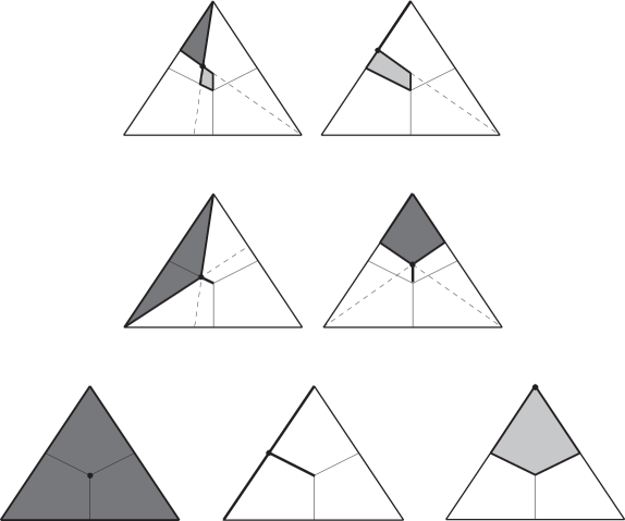
Figure 1: Pictures of $\uparrow\!\!x$ and $\downarrow\!\!x$ for $x\in\Delta^{3}$.

3.2 Quantum states

Let $\mathcal{H}^{n}$ denote an $n$-dimensional complex Hilbert space with specified inner product $\langle\cdot|\cdot\rangle.$

Definition 3.6

A quantum state is a density operator ${\rho:\mathcal{H}^{n}\rightarrow\mathcal{H}^{n}}$, i.e., a self-adjoint, positive, linear operator with $\mathrm{tr}(\rho)=1.$ The quantum states on $\mathcal{H}^{n}$ are denoted $\Omega^{n}$.

Definition 3.7

A quantum state $\rho$ on $\mathcal{H}^{n}$ is pure if

$$\mathrm{spec}(\rho)\subseteq\{0,1\}.$$

The set of pure states is denoted $\Sigma^{n}$. They are in bijective correspondence with the one dimensional subspaces of $\mathcal{H}^{n}.$

Classical states are distributions on the set of pure states $\max(\Delta^{n}).$ By Gleason’s theorem[8], an analogous result holds for quantum states: Density operators encode distributions on the set of pure states $\Sigma^{n}$ up to equivalent behavior under measurements.

Definition 3.8

A quantum observable is a self-adjoint linear operator ${e:\mathcal{H}^{n}\rightarrow\mathcal{H}^{n}}.$

If our knowledge about the state of the system is represented by density operator $\rho$, then quantum mechanics predicts the probability that a measurement of observable $e$ yields the value $\lambda\in\mathrm{spec}(e)$. It is

$$\mathrm{pr}(\rho\rightarrow e_{\lambda}):=\mathrm{tr}(p_{e}^{\lambda}\cdot\rho),$$

where $p_{e}^{\lambda}$ is the projection corresponding to eigenvalue $\lambda$ and $e_{\lambda}$ is its associated eigenspace in the spectral representation of $e$.

Definition 3.9

Let $e$ be an observable on $\mathcal{H}^{n}$ with $\mathrm{spec}(e)=\{1,\ldots,n\}.$ For a quantum state $\rho$ on $\Omega^{n}$,

$$\mathrm{spec}(\rho|e):=(\mathrm{pr}(\rho\rightarrow e_{1}),\ldots,\mathrm{pr}(\rho\rightarrow e_{n}))\in\Delta^{n}.$$

For the rest of the paper, we assume that all observables $e$ have $\mathrm{spec}(e)=\{1,\ldots,n\}.$ For our purposes it is enough to assume $|\mathrm{spec}(e)|=n$; the set $\{1,\ldots,n\}$ is chosen for the sake of aesthetics. Intuitively, then, $e$ is an experiment on a system which yields one of $n$ different outcomes; if our a priori knowledge about the state of the system is $\rho$, then our knowledge about what the result of experiment $e$ will be is $\mathrm{spec}(\rho|e).$ Thus, $\mathrm{spec}(\rho|e)$ determines our ability to predict the result of the experiment $e$.

So what does it mean to say that we have more information about the system when we have $\sigma\in\Omega^{n}$ than when we have $\rho\in\Omega^{n}$? It could mean that there is an experiment $e$ which (a) serves as a physical realization of the knowledge each state imparts to us, and (b) that we have a better chance of predicting the result of $e$ from state $\sigma$ than we do from state $\rho$. Formally, (a) means that $\mathrm{spec}(\rho)=\mathrm{Im}(\mathrm{spec}(\rho|e))$ and $\mathrm{spec}(\sigma)=\mathrm{Im}(\mathrm{spec}(\sigma|e))$, which is equivalent to requiring $[\rho,e]=0$ and $[\sigma,e]=0$, where $[a,b]=ab-ba$ is the commutator of operators.

Definition 3.10

Let $n\geq 2$. For quantum states $\rho,\sigma\in\Omega^{n}$, we have $\rho\sqsubseteq\sigma$ iff there is an observable $e:\mathcal{H}^{n}\rightarrow\mathcal{H}^{n}$ such that $[\rho,e]=[\sigma,e]=0$ and $\mathrm{spec}(\rho|e)\sqsubseteq\mathrm{spec}(\sigma|e)$ in $\Delta^{n}$.

This is called the spectral order on quantum states.

Theorem 3.11

$(\Omega^{n},\sqsubseteq)$ is a dcpo with maximal elements

$$\mathrm{max}(\Omega^{n})=\Sigma^{n}$$

and least element $\bot=I/n$, where $I$ is the identity matrix.

There is one case where the spectral order can be described in an elementary manner.

Example 3.12

As is well-known, the $2\times 2$ density operators can be represented as points on the unit ball in ${\mathbb{R}}^{3}:$

$$\Omega^{2}\simeq\{(x,y,z)\in{\mathbb{R}}^{3}:x^{2}+y^{2}+z^{2}\leq 1\}.$$

For example, the origin $(0,0,0)$ corresponds to the completely mixed state $I/2$, while the points on the surface of the sphere describe the pure states. The order on $\Omega^{2}$ then amounts to the following: $x\sqsubseteq y$ iff the line from the origin $\bot$ to $y$ passes through $x$.

Like the Bayesian order on $\Delta^{n}$, the spectral order on $\Omega^{n}$ can also be characterized in terms of symmetries and projections. In its symmetric formulation, unitary operators on $\mathcal{H}^{n}$ take the place of permutations on $\{1,\ldots,n\}$, while the projective formulation of $(\Omega^{n},\sqsubseteq)$ shows that each classical projection $p_{i}:\Delta^{n+1}\rightharpoonup\Delta^{n}$ is actually the restriction of a special quantum ‘projection’ $\Omega^{n+1}\rightharpoonup\Omega^{k}$ with $k=n$.

3.3 The logics of Birkhoff and von Neumann

The logics of Birkhoff and von Neumann[2] consist of the propositions one can make about a physical system. Each proposition takes the form “The value of observable $e$ is contained in $E\subseteq\mathrm{spec}(e).$” For classical systems, the logic is $\mathcal{P}\{1,\ldots,n\}$, while for quantum systems it is $\mathbb{L}^{n}$, the lattice of (closed) subspaces of $\mathcal{H}^{n}.$ In each case, implication of propositions is captured by inclusion, and a fundamental distinction between classical and quantum – that there are pairs of quantum observables whose exact values cannot be simultaneously measured at a single moment in time – finds lattice theoretic expression: $\mathcal{P}\{1,\ldots,n\}$ is distributive; $\mathbb{L}^{n}$ is not.

We now establish the relevance of the domains $\Delta^{n}$ and $\Omega^{n}$ to theoretical physics: The classical and quantum logics can be derived from the Bayesian and spectral orders using the same order theoretic technique.

Definition 3.13

An element $x$ of a dcpo $D$ is irreducible when

$$\bigwedge(\uparrow\!\!x\cap\max(D))=x$$

The set of irreducible elements in $D$ is written $\mbox{Ir}(D).$

The order dual of a poset $(D,\sqsubseteq_{D})$ is written $D^{*}$; its order is $x\sqsubseteq y\Leftrightarrow y\sqsubseteq_{D}x.$

Theorem 3.14

For $n\geq 2$, the classical lattices arise as

$$\mathrm{Ir}(\Delta^{n})^{*}\simeq\mathcal{P}\{1,\ldots,n\}\setminus\{\emptyset\},$$

and the quantum lattices arise as

$$\mathrm{Ir}(\Omega^{n})^{*}\simeq\mathbb{L}^{n}\setminus\{0\}.$$

It is worth pointing out that these logics consist exactly of the states traced out by the motion of a searching process on each of the respective domains. To illustrate, let ${p_{i}^{+}:\Delta^{n}\rightarrow\Delta^{n}}$ for $1\leq i\leq n$ denote the result of first applying the Bayesian projection $p_{i}$ to a state, and then reinserting a zero in place of the element removed. Now, beginning with $\bot\in\Delta^{n}$, apply one of the $p_{i}^{+}$. This projects away a single outcome from $\bot$, leaving us with a new state. For the new state obtained, project away another single outcome; after $n-1$ iterations, this process terminates with a pure state $e_{i}$, and all the intermediate states comprise a path from $\bot$ to $e_{i}$. Now imagine all the possible paths from $\bot$ to a pure state which arise in this manner. This set of states is exactly $\mathrm{Ir}(\Delta^{n}).$ (See Figure 2).

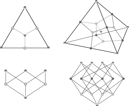
Figure 2: The irreducibles of $\Delta^{3}$ and $\Delta^{4}$ with their corresponding Hasse diagrams.

3.4 Entropy

The formal notion of information content studied in measurement is broad enough in scope to capture Shannon’s idea from information theory, as well as von Neumann’s conception of entropy from quantum mechanics.

Theorem 3.15

Shannon entropy

$$\mu x=-\sum_{i=1}^{n}x_{i}\log x_{i}$$

is a measurement of type $\,\Delta^{n}\rightarrow[0,\infty)^{*}.$

A more subtle example of a measurement on classical states is the retraction $r:\Delta^{n}\rightarrow\Lambda^{n}$ which rearranges the probabilities in a classical state into descending order.

Theorem 3.16

von Neumann entropy

$$\sigma\rho=-\mathrm{tr}(\rho\log\rho)$$

is a measurement of type $\Omega^{n}\rightarrow[0,\infty)^{*}.$

Another natural measurement on $\Omega^{n}$ is the map ${q:\Omega^{n}\rightarrow\Lambda^{n}}$ which assigns to a quantum state its spectrum rearranged into descending order. It is an important link between classical and quantum information theory.

By combining the quantitative and qualitative aspects of information, we obtain a highly effective method for solving a wide range of problems in the sciences. As an example, consider the problem of rigorously proving the statement “there is more information in the quantum than in the classical.”

The first step is to think carefully about why we say that the classical is contained in the quantum; one reason is that for any observable $e$, we have an isomorphism

$$\Omega^{n}|e=\{\rho\in\Omega^{n}:[\rho,e]=0\}\simeq\Delta^{n}$$

between the spectral and Bayesian orders. That is, each classical state can be assigned to a quantum state in such a way that information is conserved:

conservation of information

$=$

 (qualitative conservation) + (quantitative conservation)

$=$

          (order embedding) + (preservation of entropy).

This realization, that both the qualitative and the quantitative characteristics of information are preserved in passing from the classical to the quantum, solves the problem.

Theorem 3.17

Let $n\geq 2$. Then

1. There is an order embedding $\phi:\Delta^{n}\rightarrow\Omega^{n}$ with ${\sigma\circ\phi=\mu.}$

2. For any $m\geq 2$, there is no order embedding ${\phi:\Omega^{n}\rightarrow\Delta^{m}}$ with ${\mu\circ\phi=\sigma.}$

Part (ii) is true for any pair of measurements $\mu$ and $\sigma$. The proof is fun: If (ii) is false, then $\phi$ restricts to an injection of $\max(\Omega^{n})$ into $\max(\Delta^{n})$, using $\ker\mu\subseteq\max(\Delta^{n})$ and $\ker\sigma=\max(\Omega^{n})$. But no such injection can actually exist: $\max(\Omega^{n})$ is infinite, $\max(\Delta^{n})$ is not.

4 Axioms for partiality

We have already mentioned that the domains $(\Delta^{n},\sqsubseteq)$ and $(\Omega^{n},\sqsubseteq)$ are not continuous. The easiest way to see why is to take note of the fact that the Bayesian order on $\Delta^{n}$ is degenerative: If $x\sqsubseteq y$, then

$$y_{i}=y_{j}>0\Rightarrow x_{i}=x_{j}>0.$$

Using this property, it is easy to show that the only approximation of a state like $(1/2,1/2,0)$ is $\bot$ by construct an increasing sequence $(y_{n})$ whose last two components are equal such that ${(1/2,1/2,0)\sqsubseteq e_{1}=\bigsqcup y_{n}}$. Nevertheless, these domains do possess a notion of approximation.

Definition 4.1

Let $D$ be a dcpo. For $x,y\in D$, we write $x\ll y$ iff for all directed sets $S\subseteq D$,

$$y=\bigsqcup S\Rightarrow(\exists s\in S)\,x\sqsubseteq s.$$

The approximations of $x\in D$ are

$$\mathord{\mbox{\makebox[0.0pt][l]{\raisebox{-1.72218pt}{$\downarrow$}}$\downarrow$}}x:=\{y\in D:y\ll x\},$$

and $D$ is called exact if $\mathord{\mbox{\makebox[0.0pt][l]{\raisebox{-1.72218pt}{$\downarrow$}}$\downarrow$}}x$ is directed with supremum $x$ for all $x\in D$.

Notice that the difference between this definition and the previous is that $\sqsubseteq$ has been replaced with ‘$=$’. A continuous dcpo is exact, for example, and in that case, the classical definition of $\ll$ is equivalent to the one above. The following is proven in[6]:

Theorem 4.2

$(\Delta^{n},\sqsubseteq)$ and $(\Omega^{n},\sqsubseteq)$ are exact.

To hint at why, we can approximate any $x\in\Delta^{n}$ using the straight line path $\pi_{\bot x}:[0,1]\rightarrow\Delta^{n}$ from $\bot$ to $x$,

$$\pi_{\bot x}(t)=(1-t)\bot+tx.$$

It is Scott continuous with $\pi_{\bot x}(t)\ll x$ for $t<1$. The analogous result holds for $\Omega^{n}.$

Definition 4.3

An element $x\in D$ is a coordinate if either $x\in\mathrm{Ir}(D)$ or $x\in\mathord{\mbox{\makebox[0.0pt][l]{\raisebox{-1.72218pt}{$\downarrow$}}$\downarrow$}}\mathrm{Ir}(D).$

In the case of $\Delta^{n}$ and $\Omega^{n}$, a coordinate is either a proposition or an approximation of a proposition. Equivalently, a coordinate is a state on one of the lines joining $\bot$ to a proposition.

Theorem 4.4

Each state is the supremum of coordinates.

The result above, proven in[5], holds for both $\Delta^{n}$ and $\Omega^{n}$. We do not expect all domains to have this property, but the role of partiality in defining ‘coordinate’ – as either an irreducible or an approximation of an irreducible – may be worth taking note of in trying to develop a general and useful set of axioms for the description of partiality. Ideally, these axioms will

• generalize continuous domains,

• include $(\Delta^{n},\sqsubseteq)$ and $(\Omega^{n},\sqsubseteq)$ as examples,

• aid in the description of a fundamental topology, which will be equivalent to the Scott topology in the case of continuous dcpo’s, and

• be relatable to implicit uses of the notion in physics, such as ‘dynamics’ (i.e., causality relations on light cones[3]).

The interested reader will notice that exact dcpo’s definitely satisfy the first two criteria. We do not know about the other two (or even what the last one may mean). Nevertheless, we hope this paper will serve as a useful guide for those intent on looking.

References

References

- [1] S. Abramsky and A. Jung. Domain theory. In S. Abramsky, D. M. Gabbay, T. S. E. Maibaum, editors, Handbook of Logic in Computer Science, vol. III. Oxford University Press, 1994.
- [2] G. Birkhoff and J. von Neumann. The logic of quantum mechanics. Annals of Mathematics, 37, 823–843, 1936.
- [3] L. Bombelli, J. Lee, D. Meyer and R. Sorkin. Spacetime as a causal set. Physical Review Letters, 59, 521–524, 1987.
- [4] B. Coecke, D. J. Moore, and A. Wilce, editors, Current research in operational quantum logic: Algebras, categories, languages. Kluwer Academic Publishers, 2000.
- [5] B. Coecke. Entropic geometry from logic. Proceedings of Mathematical Foundations of Programming Semantics 19, Electronic Notes in Theoretical Computer Science, vol. 83, 2003. arXiv:quant-ph/0212065
- [6] B. Coecke and K. Martin. A partial order on classical and quantum states. Oxford University Computing Laboratory, Research Report PRG-RR-02-07, August 2002. http://web.comlab.ox.ac.uk/oucl/ publications/tr/rr-02-07.html
- [7] R. Engelking. General topology. Polish Scientific Publishers, 1977.
- [8] A. M. Gleason. Measures on the closed subspaces of a Hilbert space. Journal of Mathematics and Mechanics, 6, 885–893, 1957.
- [9] K. Martin. A foundation for computation. Ph.D. Thesis, Department of Mathematics, Tulane University, 2000.
- [10] K. Martin. The measurement process in domain theory. Proceedings of the International Colloquium on Automata, Languages and Programming (ICALP), Lecture Notes in Computer Science, Springer-Verlag, vol. 1853, 2000.
- [11] K. Martin. Fractals and domain theory. Mathematical Structures in Computer Science, Cambridge University Press, to appear.
- [12] P. Odifreddi. Classical recursion theory. Studies in Logic and the Foundations of Mathematics, vol. 125, Elsevier Science, North Holland, 1989.
- [13] D. Scott. Outline of a mathematical theory of computation. Technical Monograph PRG-2, Oxford University Computing Laboratory, 1970.