E-mail: jalar@mai.liu.se
Department of Mathematics, University of Utrecht, Box 80010, NL-3508 TA Utrecht, The Netherlands
EURANDOM, P.O. Box 513, NL-5600 MB Eindhoven, The Netherlands
Entanglement and quantum nonlocality
Bell’s inequality and the coincidence-time loophole
Abstract
This paper analyzes effects of time-dependence in the Bell inequality. A generalized inequality is derived for the case when coincidence and non-coincidence [and hence whether or not a pair contributes to the actual data] is controlled by timing that depends on the detector settings. Needless to say, this inequality is violated by quantum mechanics and could be violated by experimental data provided that the loss of measurement pairs through failure of coincidence is small enough, but the quantitative bound is more restrictive in this case than in the previously analyzed “efficiency loophole.”
pacs:
03.65.UdThe Bell inequality [1] and its descendants (see e.g., ref. [2]) have been the main argument on the EPR-paradox [3, 4] for the last forty years. A new research field of ‘experimental metaphysics’ has formed, where the goal is to show that the concept of local realism is inconsistent with quantum mechanics, and ultimately with the real world. The experiments which have been performed to verify this have not been completely conclusive, but they point in a certain direction: Nature cannot be described by a local realist model. The reason for saying “not been completely conclusive” is the existence of certain “loopholes” in these experiments. For example, the so-called “efficiency loophole” is present in all photonic experiments performed to date including Aspect et al [5, 6, 7] and Weihs et al [8]. This is usually dealt with using the “no-enhancement” assumption, which would not be needed if the efficiency would be high enough (see refs [9, 10, 11, 12, 13, 14]). Recently, there was a 100% efficiency experiment by Rowe et al [16], but that experiment does not enforce strict locality.
This paper is motivated by recent claims (e.g., ref. [15]) that time-dependence has been omitted in the Bell inequality. A close examination of the presented counterexample(s) show that they are in fact nonlocal; the probability measure used depends on both detector parameters and is thus not local in the Bell sense. In fact, there is no problem in using the measurement time as a hidden variable in a truly local Bell setting. Nevertheless, while working through the details we found that timing issues may indeed play a role, even in a local model. The present analysis incorporates this in a generalized Bell inequality, for which the reader may find that certain bounds are higher than naïvely expected. We will also note that the loophole can be closed with relative ease in experiments, and indeed is in some modern experiments.
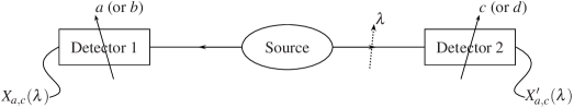
The situation is as follows: in the standard Bell setup (see Fig. 1), we want to take into account that the time-correlation is not perfect between results at one site and results at the other. Usually, there is a “coincidence window” in which events are counted as being “simultaneous,” i.e., belonging to the same pair so that they contribute to the correlation, even when there is a finite (i.e., nonzero) time between them111For simplicity we assume that the two detectors are stationary in the same inertial frame, and use that frame to determine simultaneity.. There is a possibility that, in this type of setup, the local setting may change the time at which the local event happens. And this would have implications; a certain local event may be simultaneous with a remote event, or not, depending on the local detector setting. The result will be that the simultaneity of two detection events will depend on both settings, even though the underlying physical processes that control this are completely local. We will examine this situation in detail and derive precise bounds for violation of the appropriate Bell inequality.
To perform the intended formal examination of this, we need to put the hidden-variable model into formal language. We arrive at a probabilistic model 222It may seem that we only discuss the “deterministic” case here, but a generalization to the “stochastic” case is straightforward and will not be done here.. Here, the hidden variable is a point in a “sample space” , the space of all possible values of the hidden variable. The measurement results are described by random variables (RVs) which take their values in the value space , usually taken as in the spin- case (see Fig. 1).
There is a probability measure on the space , used to calculate the probabilities of the different outcomes and the expectation value , where
| (1) |
suppressing the parentheses. We then obtain the expectation of the product of the results as , usually denoted “correlation” in this context 333The reason for this is that in the simplest case and , and then the correlation is precisely . Here, this terminology will be retained even for cases when this ceases to be valid, as it has become standard in this context. Finally, after using locality only four RVs remain; , , and , see below. Now, we have
Theorem 1 (The Clauser-Horne-Shimony-Holt (CHSH) inequality) The following three prerequisites are assumed to hold except at a null set:
-
(i)
Realism. Measurement results can be described by probability theory, using two families of RVs, e.g.,
(i) -
(ii)
Locality. A measurement result should be independent of the remote setting, e.g.,
(ii) -
(iii)
Measurement result restriction. The results may only range from to ,
(iii)
Then
| (2) |
The proof consists of simple algebraic manipulations inside each of the two expressions on the right hand side, followed by application of the triangle inequality on each expression.
Previous treatments have discussed several loopholes in this inequality, but the most similar issue to the present is the “detector efficiency” problem. A simple formalism to use is that of ref. [13], where inefficient detectors, or in more general terms, inefficient measurement setups are modeled by having the measurement-result RVs undefined at points in where no detection occurs. This means that, e.g., the RVs and will only be defined at subsets of denoted and , resp.. The averaging must now be restricted to the set where the RV in question is defined, and the probability measure adjusted accordingly. In the language of probability theory we need the conditional expectation value
| (3) |
using the conditional probability measure
| (4) |
In the detector efficiency case, the first correlation in the CHSH inequality then is , the expectation of conditioned on both factors in the product being defined (that both results are observed). This is the correlation that would be obtained from an experimental setup where the coincidence counters are told to ignore single particle events.
In the present case, there is a slight difference. In a hidden-variable model, the detection times and at the two sites can be described as RVs that depend on the settings, e.g.,
| (5) |
A “coincidence” then occurs when the two times differ by less than some predetermined time interval . In mathematical language this corresponds to saying that coincidences occur for certain values of the hidden variable , e.g., at the settings and , values in the set
| (6) |
In the following, we will concentrate on the set (but it does help to remember its origin), and this set can vary depending on both detector settings. Note that no assumption has yet been made on the locality of the detection times and at the two sites; they may depend on both settings. Remember that we are concentrating on the resulting statistics of , , , and here, and only use the times to find coincidences. If it makes the reader feel better, he/she may use an implicit locality assumption ( and ), but that is of no consequence below.
The first correlation in the CHSH inequality then is , the expectation of conditioned on coincidences for the settings and . The original CHSH inequality is no longer valid, and the reason can be seen in the start of the proof where one wants to add
| (7) |
The integrals on the right-hand side cannot easily be added when , since we are taking expectations over different ensembles and , with respect to different probability measures.
The problem here is that the ensemble on which the correlations are evaluated changes with the settings, while the original Bell inequality requires that they stay the same. In effect, the Bell inequality only holds on the common part of the four different ensembles , , , and , i.e., for correlations of the form
| (8) |
Unfortunately our experimental data comes in the form
| (9) |
so we need an estimate of the relation of the common part to its constituents:
| (10) |
This is a purely theoretical construct, not available in experimental data, but we will relate it to experimental data below. Anyhow, fixing this relative size, we can prove
Theorem 2 (The CHSH inequality with coincidence restriction) The prerequisites (i–iii) of Theorem 1 are assumed to hold except at a null set, as is
-
(iv)
Coincident events. Correlations are obtained on subsets of , namely on
(iv)
Then
| (11) |
Proof. The proof consists of two steps; the first part is similar to the proof of Theorem 1, using the intersection
| (12) |
on which coincidences occur for all relevant settings. This ensemble may be empty, but only when and then the inequality is trivial, so can be assumed in the rest of the proof. Now (i–iii) yields
| (13) |
The second step is to translate this into an expression with and so on. For brevity, let and denote “set complement” by . Then, and
| (14) |
We now have
| (15) |
which, together with ineq. (13) and the triangle inequality,
yields the desired result after some simple manipulations.
Let us now relate this to experimental quantities. In this context, the quantity of greatest interest is the probability of coincidence:
| (16) |
We now have
| (17) |
because (Bonferroni)
| (18) |
and
| (19) |
Putting this into our modified CHSH inequality we arrive at
| (20) |
The bound for violation by quantum mechanics here is , which is considerably higher than the corresponding value for the detector-efficiency case, .
Let us see whether this bound is necessary and sufficient. At the same time, we answer the question if it would be possible to lower the bound by putting further natural constraints on the model. This will be done by construction of an ad hoc model that will give the quantum predictions at the settings , , , and , and the additional natural constraints are: it will only use local data, even for timing; the marginal distributions are correct; there is full correlation if the settings are equal at the two sites; and the coincidence probability is the same at our specified pairs of settings.
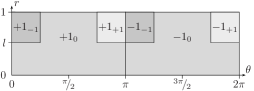
The model is as follows: the hidden variable is a pair of coordinates, uniformly distributed over the rectangle indicated in Fig. 2. The local detector setting corresponds to a shift in the -direction of the pattern, with wrap-around when necessary. The result is obtained according to the diagram (the subscript is the detection time which can be or 0). To make the behaviour interesting we choose to be 3/2, so that a time-difference of zero or one time unit(s) is a coincidence while a time-difference of two time units will not be a coincidence.
For example, for the settings and at the two sites, there will be coincidences at the s indicated in Fig. 3, so that the probability of coincidence is , while the probability of getting or is . For the settings and at the two sites, the probability of coincidence would again be , while the probability of getting or would only be , so that
| (21) |
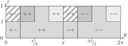
Setting , i.e., we obtain
| (22) |
which saturates the derived coincidence probability bound. This model does what we have asked so far, especially, it violates the Bell inequality maximally. The model does not have constant coincidence probability for all angular settings but can be modified so that it does 444The relative delays in our ad hoc model vary in probability, but this can also be fixed, introducing some additional complexity.. Furthermore, the interference pattern is not sinusoidal, and delays are discrete, but this will be a subject of further research (see e.g., ref. [14]).
We have seen that a useful Bell inequality does hold even if the detection time is allowed to depend on the settings, if sufficiently many events are simultaneous. That the inequality needs to be modified when events are allowed to drop from the statistics is not surprising but to be expected, cf. previous analysis in the low-efficiency case. It is perhaps more surprising that the amount of coincidences needs to be higher in this case than in the efficiency case. The reason for this is that the set of coincidences factors in the efficiency case, i.e., (see ref. [13]), while here the set cannot be factored. Thus, the present treatment is a proper generalization of the previous results. A major remaining challenge is to extend the analysis to the situation when coincidence, detection and memory loopholes (see refs. [17, 18, 19]) are all present.
Several modern experiments are not affected by this loophole, such as the ion trap experiment by Rowe et al [16], because there, all experimental runs produce coincidences (although locality is not strictly enforced). Also, the “event-ready” experiment proposed in ref. [20] removes the coincidence loophole (see also ref. [21]). Such an experiment uses a tri-partite system and a third detector located, e.g., near the source as an indicator that there is a pair being emitted. A detection there would then be independent of the settings of the distant detectors and would give the timing information needed to remove the coincidence loophole. In the case of pulsed optical experiments, one can use the natural assumption that the setting-dependent delays described by and do not depend on the relation between pulse length and pulse spacing. Then, if the pulse (e.g., the driving pulse of a parametric downconverter) is short in comparison to the pulse spacing, one can assume that any delays that occur will not delay photons from the time-window of one pulse to the next, or at least that this will happen only with very low probability. Now, the driving pulse will provide a well-defined, pre-determined coincidence window and this will remove the coincidence loophole. In both the latter approaches a lowered efficiency may remain, but using an event-ready experiment or a pulsed source (with the above two natural assumptions) will enable use of the previous lower bound, e.g., from ref. [13].
In conclusion, we have shown that the coincidence loophole can be significantly more damaging than the well-studied detection problem. Fortunately, the damage can be quantified and in some cases, repaired. The results underline the importance of eliminating post-selection in future experiments.
Acknowledgements.
J.-Å. L. was financially supported by the Swedish research council. R. D. G. was partially funded by project RESQ (IST-2001-37559) of the IST-FET programme of the European Union.References
- [1] J. S. BELL, Physics 1, 195 (1964).
- [2] J. F. CLAUSER, M. A. HORNE, A. SHIMONY, and R. A. HOLT, Phys. Rev. Lett. 23, 880 (1969).
- [3] A. EINSTEIN, B. PODOLSKY, and N. ROSEN, Phys. Rev. 47, 777 (1935).
- [4] D. BOHM and Y. AHARONOV, Phys. Rev. 108, 1070 (1957).
- [5] A. ASPECT, P. GRANGIER, and G. ROGER, Phys. Rev. Lett. 47, 460 (1981).
- [6] A. ASPECT, P. GRANGIER, and G. ROGER, Phys. Rev. Lett. 49, 91 (1982).
- [7] A. ASPECT, J. DALIBARD, and G. ROGER, Phys. Rev. Lett. 49, 1804 (1982).
- [8] G. WEIHS et al., Phys. Rev. Lett. 81, 5039 (1998).
- [9] P. PEARLE, Phys. Rev. D 2, 1418 (1970).
- [10] J. F. CLAUSER and M. A. HORNE, Phys. Rev. D 10, 526 (1974).
- [11] A. GARG and N. D. MERMIN, Phys. Rev. D 35, 3831 (1987).
- [12] A. SHIMONY, Search for a naturalistic world view (Cambridge Univ. Press, Cambridge, 1993), Vol. II.
- [13] J.-Å. LARSSON, Phys. Rev. A 57, 3304 (1998).
- [14] J.-Å. LARSSON, Phys. Lett. A 256, 245 (1999).
- [15] K. HESS and W. PHILIPP, Proc. Nat. Acad. Sci. USA 98, 14224 (2001).
- [16] M. A. ROWE et al., Nature (London) 409, 791 (2001).
- [17] R. D. GILL, in Mathematical Statistics and Applications: Festschrift for Constance van Eeden, Vol. 42 of IMS Lecture Notes – Monograph Series, edited by M. Moore, S. Froda, and C. Léger (Institute of Mathematical Statistics, Beachwood, Ohio, 2003), pp. 133–154, quant-ph/0110137.
- [18] R. D. GILL, in Proceedings of ”Foundations of Probability and Physics - 2”, Vol. 5 of Math. Modelling in Phys., Engin., and Cogn. Sc. (Växjö Univ. Press, Växjö, Sweden, 2003), pp. 179–206, quant-ph/0301059.
- [19] R. D. GILL, to appear in proceedings of ”Quantum Probability and Infinite Dimensional Analysis”, Greifswald, 2003 (World Scientific), quant-ph/0307217.
- [20] J. S. BELL, J. de Phys. Colloque C2, Tome 42, 41 (1981).
- [21] M. ZUKOWSKI, A. ZEILINGER, M. A. HORNE, and A. K. EKERT, Phys. Rev. Lett. 71, 4287 (1993).