PHYSICS OF SINGULAR POINTS IN QUANTUM MECHANICS

Abstract

Defects or junctions in materials serve as a source of interactions for particles, and in idealized limits they may be treated as singular points yielding contact interactions. In quantum mechanics, these singularities accommodate an unexpectedly rich structure and thereby provide a variety of physical phenomena, especially if their properties are controlled properly. Based on our recent studies, we present a brief review on the physical aspects of such quantum singularities in one dimension. Among the intriguing phenomena that the singularities admit, we mention strong vs weak duality, supersymmetry, quantum anholonomy (Berry phase), and a copying process by anomalous caustics. We also show that a partition wall as a singularity in a potential well can give rise to a quantum force which exhibits an interesting temperature behavior characteristic to the particle statistics.

1 Introduction

If a system contains an object (or subsystem) different from its surroundings, and if the object is very small compared to the size of the system, then one may regard it as a ‘singularity’ in the system to a first approximation. Such an object may be given by an isolated region forming a dot, or it may consist of a planar region forming a wall in the system. In view of the negligible size of the object, we may study the physical property of the system by considering a point singularity interacting with particles such as electrons by contact interaction. The outcome will furnish a basis for studying the physics of systems with singular objects given by quantum dots or junctions in semiconductors, where the finite size effect may be considered as secondary to the zero size effect. This analysis is also useful for analyzing systems from a long range point of view, where the singular object is reduced to a point (or a plane without thickness) in effect.

In classical mechanics, a singular point will have no characteristics and is basically trivial. In quantum mechanics, in contrast, it has been known that there are many, distinct singular points allowed, and if the system is one dimensional (i.e., line) they form a $U(2)$ family [1, 2]. The distinction among them lies in the connection conditions at the singularity obeyed by the wave functions, which can lead to entirely different physical consequences depending on the choice of the singularity. Our interest then is to see how these singular points can be characterized mathematically, and to find what type of physical phenomena can be expected in systems with particles interacting with the $U(2)$ family of singularities if they are manipulated appropriately. The aim of the present paper is to provide a review of our investigations on these matters, and thereby to point out that, once a controllable singularity is introduced in the otherwise free system on a line, then there appear many physically interesting properties, such as duality, anholonomy (Berry phase), supersymmetry and a copying process by quantum anomalous caustics. We also mention a statistical aspect of systems with a singularity, which is the emergence of a force on a partition wall (regarded as singularity). The force is generated by distinct boundary conditions and exhibits an interesting dependence — characteristic to the particle statistics (bosons or fermions) — on the temperature and the particle number of the system. Our consideration is restricted only to one dimensional systems, but the essential features of quantum singularities found here will also persist in higher dimensional systems.

This paper is organized as follows. After the Introduction, we briefly recall in section 2 how the $U(2)$ family of singularities appear in quantum mechanics on a line. The physical meaning of the matrix notation used to characterize the family of singularities is then discussed in section 3. Sections 4 and 5 are devoted to the physical phenomena afforded under the presence of the singularities mentioned above. Section 6 discusses the quantum force on a partition wall and its temperature behavior. Finally, we give our discussions in section 7.

2 Quantum Description of a Singular Point on a Line

Suppose that there is a point singularity, say, at $x=0$ on a line $-\infty<x<\infty$. If the singularity is not accompanied by a potential, then our Hamiltonian is the free one,

$$H=-{{\hbar^{2}}\over{2m}}{{d^{2}}\over{dx^{2}}},$$ (1)

and the singularity will just impose a certain connection condition for wave functions at $x=0$. The connection condition arises from the requirement of the unitarity of the system, which is ensured if the probability current $j(x)=-{{i\hbar}\over{2m}}\left((\psi^{*})^{\prime}\psi-\psi^{*}\psi^{\prime}\right)(x)$ is continuous at the singularity, $j(+0)=j(-0)$. This can be shown to be equivalent to the connection condition [3, 4]

$$(U-I)\Psi+iL_{0}(U+I)\Psi^{\prime}=0,$$ (2)

where $U\in U(2)$ is called characteristic matrix, $L_{0}\neq 0$ is a real (arbitrary) constant and

$$\Psi=\left(\begin{array}[]{c}{\psi(+0)}\\ {\psi(-0)}\end{array}\right),\quad\Psi^{\prime}=\left(\begin{array}[]{c}{\psi^{\prime}(+0)}\\ {-\psi^{\prime}(-0)}\end{array}\right),$$ (3)

are vectors defined from the boundary values of the wave function $\psi(\pm 0)=\lim_{x\to\pm 0}\psi(x)$ and their derivatives. In other words, imposing the probability conservation as the sole requirement in quantum mechanics, we find the $U(2)$ freedom in specifying the connection condition, that is, there exist the $U(2)$ family of singularities possessing different connection conditions on a line. For instance, if we choose $U=\sigma_{1}$ (where $\sigma_{i}$ are Pauli matrices), the connection condition (2) reduces to $\psi(+0)=\psi(-0)$, $\psi^{\prime}(+0)=\psi^{\prime}(-0)$, which represents the ‘free system’ — no actual singularity at all. On the other hand, the choice $U=-I$ gives the Dirichlet condition $\psi(+0)=\psi(-0)=0$ while $U=I$ gives the Neumann condition $\psi^{\prime}(+0)=\psi^{\prime}(-0)=0$.

The last two choices provide two examples of connection conditions that prohibit the probability flow at the singularity. All of these conditions represent, physically, an ‘infinite’ partition wall with distinct characters. The general singularities that do not allow the probability flow are obtained by requiring $j(+0)=j(-0)=0$, and the characteristic matrices that meet this requirement are given by diagonal $U\in U(2)$. These form the so-called ‘separated subfamily’ $U(1)\times U(1)$ in the $U(2)$ family, for which the connection condition (2) reduces to the boundary condition,

$$\psi(+0)+L(\theta_{+})\psi^{\prime}(+0)=0,\qquad\psi(-0)+L(\theta_{-})\psi^{\prime}(-0)=0,$$ (4)

where

$$L(\theta_{\pm})=L_{0}\cot{{\theta_{\pm}}\over 2},$$ (5)

with $\theta_{\pm}$ being the phase parameters of ${\rm diag}\,U=(e^{i\theta_{+}},e^{i\theta_{-}})$. The Dirichlet and the Neumann conditions are obtained, respectively, by choosing $L(\theta_{\pm})=0$ and $L(\theta_{\pm})=\infty$. In passing we note that, if the singularity is a wall (an end point of a positive half line), then the condition is simply $\psi(+0)+L(\theta_{+})\psi^{\prime}(+0)=0$. An important point to be noted is that neither wave functions nor their derivatives are continuous at the singularity under a generic singularity (dot, partition or wall).

The forgoing argument applies almost unchanged to cases where the singularity arises as a divergent point of a potential, such as the Coulomb potential $V(x)=c/|x|$. The only technical modification necessary is that the boundary vectors used in the connection condition (2) must be slightly generalized as [5]

$$\Psi=\left(\begin{array}[]{c}{W[\psi,\varphi_{1}]_{+0}}\\ {W[\psi,\varphi_{1}]_{-0}}\end{array}\right),\quad\Psi^{\prime}=\left(\begin{array}[]{c}W[\psi,\varphi_{2}]_{+0}\\ -W[\psi,\varphi_{2}]_{-0}\end{array}\right)$$ (6)

with the help of reference states $\varphi_{1}$, $\varphi_{2}$ which are arbitrarily chosen to provide the self-dual Wronskians $W[\phi,\psi](x)=\phi(x)\psi^{\prime}(x)-\psi(x)\phi^{\prime}(x)$. The modification is required because wave functions (and/or their derivatives), and hence the boundary vectors (2), may diverge at the singularity under diverging potentials, while the Wronskians are always well-defined. We note that (6) is a generalization of (3), since by a suitable choice of the reference states one can regain (3) from (6) when the states $\psi$ are well-defined at the singularity.

3 Characteristic Matrix and the Spectral Space

In order to investigate the physics implied by the singularity, we introduce the parametrization [6, 7] of the characteristic matrix,

$$U=V^{-1}DV,$$ (7)

with

$$D=\left(\begin{array}[]{cc}e^{i\theta_{+}}&0\\ 0&e^{i\theta_{-}}\end{array}\right),\qquad V=e^{i{\mu\over 2}\sigma_{2}}e^{i{\nu\over 2}\sigma_{3}}$$ (8)

where $\theta_{\pm}\in[0,2\pi)$ and $\mu\in[0,\pi]$, $\nu\in[0,2\pi)$. The convenience of the parametrization may be recognized by the following observations. Notice, first, that any eigenstate $\psi(x)$ with energy $E$ remains to be an eigenstate after the transformation of the parity ${\cal P}$ or the half-reflection ${\cal R}$ defined by

$${\cal P}:\psi\rightarrow({\cal P}\psi)(x):=\psi(-x),\qquad{\cal R}:\psi\rightarrow({\cal R}\psi)(x):=[\Theta(x)-\Theta(-x)]\psi(x).$$ (9)

The only effect caused by these can be found in the change of the connection condition that the eigenstate obeys, and these are described by the corresponding change in the characteristic matrix,

$$U\buildrel{{\cal P}}\over{\longrightarrow}\sigma_{1}\,U\,\sigma_{1},\qquad U\buildrel{{\cal R}}\over{\longrightarrow}\sigma_{3}\,U\,\sigma_{3}.$$ (10)

Obviously, the same can be observed with the transformation generated by the product ${\cal Q}=i{\cal P}{\cal R}$, which implies that this remains so even under any transformation given by a linear combination of the three generators $\{{\cal P},{\cal Q},{\cal R}\}$ which form an $su(2)$ algebra, as long as it does not change the norm of the state. These general isospectral transformations induce conjugations to the matrix $U$ by $U\rightarrow W^{-1}UW$ with $W\in SU(2)$.

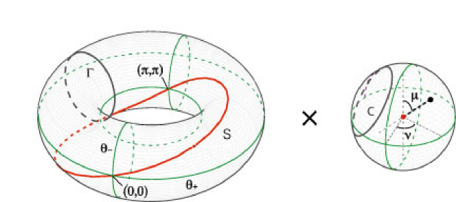
Figure 1: $U(2)$ parameter space as a product of the torus $T^{2}$ determining the spectrum (the spectral space is its half $T^{2}/Z_{2}$ which is a Möbius strip) and the isospectral sphere $S^{2}$.

Thus we learn that the decomposition (7) with (8) provides a split in the parameters into those that determine the sepctrum and those that do not, that is, $(\theta_{+},\theta_{-})$ and $(\mu,\nu)$. The spaces of these parameters are, therefore, given by the spectral torus $T^{2}$ and the isospectral sphere $S^{2}$ (see Figure 1), respectively. More precisely, we shall see soon that the spectrum is unchanged under the interchange of the parameters $\theta_{+}\leftrightarrow\theta_{-}$, and consequently the actual spectral space is given by $T^{2}/Z_{2}$ which is a Möbius strip with boundary [8].

The combinations $L(\theta_{\pm})$ given in (5) set the scale of the system and turn out to be more useful than $\theta_{\pm}$. For instance, for $L(\theta_{+})>0$ and/or $L(\theta_{-})>0$, the singularity can support the bound states $\psi_{\pm}(x)\propto e^{-|x|/L(\theta_{\pm})}$ where $L(\theta_{\pm})$ represent the effective range of the particle trapped around the singularity. The isospectral parameters $(\mu,\nu)$, on the other hand, are related to the phase shift of the wave function at the singularity and the degree of mixture of the limiting values of the wave function at $x=\pm 0$. The characterization of the parameters discussed here hold true even under a symmetric potential, $V(-x)=V(x)$.

4 Duality, Anholonomy and Supersymmetry

Having furnished a formal basis to describe a generic quantum singularity on a line, we now turn to its physics. Due to the nontrivial structure of the parameter space $U(2)$, various interesting phenomena can arise if we manipulate the parameters properly on the $U(2)$ space. Here we mention three of them, duality, anholonomy and supersymmetry, which can be readily realized from what we have already.

4.1 Duality

The invariance of the spectrum under the interchange $\theta_{+}\leftrightarrow\theta_{-}$ implies spectral duality for a pair of systems possessing singularities with the two parameters interchanged. To see how this happens, for simplicity we restrict ourselves to parity invariant singularities. Note that, since the parity transformation ${\cal P}$ induces the change (10), parity invariant singularities are characterized by those $U$ satisfying $\sigma_{1}\,U\,\sigma_{1}=U$. The general solution is given by

$$U=U(\theta_{+},\theta_{-})=e^{i(\theta_{+}P^{+}_{1}+\theta_{-}P^{-}_{1})},$$ (11)

with $P^{\pm}_{1}={{1\pm\sigma_{1}}\over 2}$, which is obtained by setting the ispospectral parameters $(\mu,\nu)=(\pi/2,0)$ in (8).

We also note that, to these parity invariant $U$ in (11) the half reflection ${\cal R}$ induces the exchange $\theta_{+}\leftrightarrow\theta_{-}$ through (10). In view of the fact that the spectrum is preserved under ${\cal R}$, we realize that if the parameters $(\theta_{+},\theta_{-})$ of the two systems are the opposite of each other, then they share the same energy spectrum. Moreover, since any eigenstate that arises under a parity invariant singularity can either be parity symmetric $\psi(-x)=\psi(x)$ or antisymmetric $\psi(-x)=-\psi(x)$, and since ${\cal R}$ swaps the parity, the corresponding eigenstates with the same energy in the two systems must have the opposite parity. Note that ${\cal R}$ is an identity operation for the special type of singularities defined by $\theta_{+}=\theta_{-}$, which are called ‘self-dual’. It follows that in the self-dual case, which is indicated by the loop $S$ in Figure 1, the entire spectrum consists of doubly (or evenly) degenerate levels consisting of pairs of parity symmetric and antisymmetric states (see Figure 2).

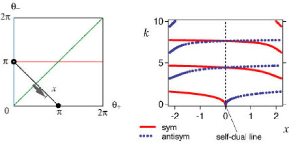
Figure 2: Spectra of two systems with a singularity placed at the centre of an infinite well, where $k$ is the momentum with the energy $E=\hbar k^{2}/(2m)$. The spectra, drawn as a function of $x$ on the torus, are identical for $x$ and $-x$, that is, for $(\theta_{+},\theta_{-})$ and $(\theta_{-},\theta_{+})$.

Now we observe that, in this parity invariant subfamily, the free system $U=\sigma_{1}$ arises at $(\theta_{+},\theta_{-})=(0,\pi)$. This suggests that we may consider ‘coupling constants’ measuring the strengths of the interaction at the singularity by

$$g_{+}(\theta_{+}):=\tan{\theta_{+}\over 2}\ ,\qquad g_{-}(\theta_{-}):=\cot{\theta_{-}\over 2}\ ,$$ (12)

which vanish, $g_{+}(0)=g_{-}(\pi)=0$, at the free point. In terms of these, we can interpret that the spectral duality holds for two systems with different coupling constants. In particular, if the parameters fulfill $\theta_{+}=\theta_{-}\pm\pi$, then we find the reciprocal behavior

$$(g_{+}(\theta_{+}),g_{-}(\theta_{-}))\buildrel{{\cal R}}\over{\longrightarrow}(-1/g_{+}(\theta_{+}),-1/g_{-}(\theta_{-})).$$ (13)

In this case, the spectral duality can occur between two systems, one with a strong coupling and the other with a weak coupling. This shows that the quantum singularity furnishes a simple example of strong vs weak coupling duality [6, 7] which is normally discussed for more complicated systems such as (supersymmetric) gauge theory.

4.2 Anholonomy

Next we turn to the opposite situation where the spectral parameters $(\theta_{+},\theta_{-})$ are fixed whereas the isospectral parameters $(\mu,\nu)$ are free to vary. If we choose the free case $(\theta_{+},\theta_{-})=(0,\pi)$ for the fixed point, the collection of such singularities provides the scale invariant subfamily, that is, they are invariant under the Weyl scale transformation,

$${\cal W}_{\lambda}:\quad\psi(x)\longrightarrow({\cal W}_{\lambda}\psi)(x):=\lambda^{1\over 2}\psi(\lambda x),$$ (14)

for real $\lambda$. For our convenience, we consider a singularity of this kind placed at the centre of in an infinite well $[-l,l]$ and impose the Dirichlet boundary condition at the ends $x=\pm l$. Then the energy eigenstates are found to be

$$\psi_{n}(x)=c_{+}(\mu)\,\xi_{n}^{+}(x)+c_{-}(\mu)e^{i\nu}\,\xi_{n}^{-}(x),$$ (15)

where

$$c_{\pm}(\mu)=\cos{\mu\over 2}\mp\sin{\mu\over 2},\qquad\xi_{n}^{\pm}(x)=\sqrt{1\over l}\sin k_{n}(x\mp l)\Theta(\pm x),$$ (16)

with $k_{n}=\left(n-{1\over 2}\right){\pi\over{2l}}$ for $n=1,2,3,\ldots$.

Now, suppose that we have some means to control the isospectral parameters $(\mu,\nu)$ adiabatically. Then we can consider a cyclic process of change along a loop $C$ on the isospectral sphere $S^{2}$ as shown in Figure 1. After completing the cycle, each eigenstate returns to the initial one modulo a phase pertinent to the state, $\psi_{n}\rightarrow e^{i\gamma(C)}\psi_{n}$. This is the phase anholonomy (or the Berry phase) and is evaluated to be

$$\gamma(C)=\oint_{C}A,\qquad A=i\langle\psi_{n}|d\psi_{n}\rangle=-{1\over 2}(1+\sin\mu)\,d\nu,$$ (17)

where $d$ is the exterior derivative in the parameter space [7]. Note that the curvature $F=dA$ is just the magnetic field of the Dirac monopole, $F=-{1\over 2}\cos\mu\,d\mu\,d\nu$.

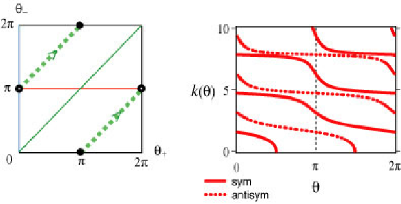
Figure 3: Spectral change along the cyclic process paralleling the self-dual loop $S$ distanced by $\pi$. Both symmetric and antisymmetric levels turn to be a lower (or higher depending on the direction) level by two after the cycle, even though the whole spectrum is unchanged.

A similar adiabatic cyclic process may also be considered on the spectral torus, instead of the isospectral sphere. For instance, we may change the spectral parameters along a loop which winds over the surface of the torus nontrivially (the simplest will be the loop $\Gamma$ in Figure 1). After completing one cycle, we find a different type of anholonomy, where each level does not return to the initial one, even though the entire spectrum as a whole is recovered. The response of the spectral change depends on the cycle one chooses; for example, if the loop is taken to be the one paralleling the self-dual loop $S$ with distance $\pi$ as shown in Figure 3, then the discrete momenta $k$ corresponding to symmetric states are given by $k=k(\theta_{+})$ while those corresponding to antisymmetric states are $k=k(\theta_{-}\pm\pi)$, where the function $k(\theta)$ is determined by

$$k(\theta)\,L_{0}\cot k(\theta)l=\tan{{\theta}\over 2}.$$ (18)

The resultant spectral change in Figure 3 shows the level anholonomy, as they shift by two after one cycle [7]. This double spiral structure of energy levels along the loop may in future be used to implement a specific physical process like the one considered for the holonomic quantum computation in systems exhibiting the Berry phase.

4.3 Supersymmetry

The double degeneracy occurring under self-dual singularities suggests that these systems may accommodate supersymmetry (SUSY). In fact, one can show that for a certain class of systems, including those with a special type of self-dual singularities, it is possible to associate SUSY without necessarily yielding degeneracy in the spectrum.

To see this, let us rewrite our system into a set of two systems each of which defined on a half line. There, we employ, instead of the wave functions $\psi(x)$ and the Hamiltonian $H$ in (1), the two-component wave functions and the corresponding Hamiltonian

$$\Psi(x)=\left(\begin{array}[]{c}{\psi_{+}(x)}\\ {\psi_{-}(x)}\end{array}\right),\qquad H=-{\hbar^{2}\over{2m}}\frac{d^{2}}{dx^{2}}\otimes I,$$ (19)

where $\psi_{\pm}(x):=\psi(\pm x)$ for $x>0$ and $I$ is the $2\times 2$ identity matrix. Our supercharge is assumed to take the form

$$Q=-i\lambda\frac{d}{dx}\otimes\sigma_{\vec{a}}+{\bf 1}\otimes\sigma_{\vec{b}},$$ (20)

where $\lambda=\hbar/2\sqrt{m}$ and

$$\sigma_{\vec{a}}=\sum_{i=1}^{3}{a_{i}\sigma_{i}},\quad\sigma_{\vec{b}}=\sum_{i=1}^{3}{b_{i}\sigma_{i}},\quad|\vec{a}|=1,\quad\vec{a}\cdot\vec{b}=0,$$ (21)

with real vectors $\vec{a}$, $\vec{b}$. The conditions (21) ensure the formal relation $2Q^{2}=H+|{\vec{b}}|^{2}$. Thus, if we absorb the constant $|{\vec{b}}|^{2}$ into the Hamiltonian (which causes only the corresponding constant energy shift), we obtain, for a set of independent supercharges $Q_{i}$ for $i=1,\ldots,N$ which are normalized properly, the standard SUSY algebra,

$$\{Q_{i},Q_{j}\}=H\,\delta_{ij}.$$ (22)

The important question we need to address at this point is whether the supercharge $Q$ leaves the given connection condition invariant, at least for energy eigenstates, because otherwise the SUSY transformation acts on states allowed under different singularities and hence the SUSY is not defined within a single system. Thus our demand for SUSY to exist is that, given a singularity specified by $U$, both the state $\Psi(x)$ and $Q\Psi(x)$ fulfill the same connection condition. To answer this question, we first note that, if the state $\Psi(x)$ fulfills the connection condition (2), then for any $W\in U(2)$ the state $W\Psi(x)$ fulfills the same connection condition with $U$ replaced by $WUW^{-1}$. This implies that, if the pair $(U,Q)$ satisfies the above demand, so does the pair $(WUW^{-1},WQW^{-1})$. Note also that $WQW^{-1}$ is again in the form (20), and hence by choosing in particular $W=V$ with $V$ appearing in the decomposition (7), we find that the pair $(D,VQV^{-1})$ also satisfies the demand. For this reason, with no loss of generality, we may assume that $U$ is diagonal. We then find, by a straightforward inspection, that the required condition is fulfilled if $\theta_{+}=\theta\neq 0$ and $\theta_{-}=\pi$ (and vice versa), and further if the supercharge takes the form

$$Q=V^{-1}\,q(\alpha,c;\theta)\,V,$$ (23)

with

$$q(\alpha,c;\theta)={}-i\lambda\frac{d}{dx}\otimes e^{-i{\alpha\over 2}\sigma_{3}}\sigma_{1}e^{i{\alpha\over 2}\sigma_{3}}{}+{\bf 1}\otimes\left[-{\lambda\over{L(\theta)}}e^{-i{\alpha\over 2}\sigma_{3}}\sigma_{2}e^{i{\alpha\over 2}\sigma_{3}}+c\,\sigma_{3}\right],$$ (24)

where $L(\theta)$ is the scale parameter defined in (5). Since $\alpha$ is arbitrary, there are two independent supercharges, i.e., the system has an $N=2$ SUSY [9, 10] as long as one of the two eigenvalues of the characteristic matrix $U$ is $-1$ and the other not $-1$.

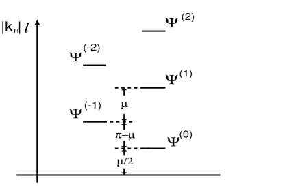
Figure 4: Energy levels of the $N=1$ SUSY system occurring under the singularity with $U=V^{-1}\sigma_{3}V$. The levels, which are dependent on $\mu$ because the boundary conditions break the parity invariance, are not degenerate unless $\mu=0$ or $\pi$.

When we put the singularity in an infinite well, then the SUSY may be found depending on the boundary conditions imposed at the ends. Various combinations, and accordingly various types of SUSY systems arise, and before we proceed we mention one of these. Consider the boundary condition

$$\psi^{\prime}_{+}(l)=0,\qquad\psi_{-}(l)=0,$$ (25)

and the singularity specified by $U=V^{-1}\sigma_{3}V$ which gives the connection condition

$$e^{i\nu}\psi_{+}(+0)-\cot{\mu\over 2}\,\psi_{-}(+0)=0,\qquad e^{i\nu}\psi_{+}^{\prime}(+0)+\tan{\mu\over 2}\,\psi_{-}^{\prime}(+0)=0.$$ (26)

Then, the system admits an $N=1$ SUSY with the supercharge $Q$ for $\vec{b}=0$ and the energy eigenstates

$$\Psi^{(n)}(x)=N^{(n)}\left(\matrix{-e^{-i\nu}\cos k_{n}(x-l)\cr\sin k_{n}(x-l)}\right),\qquad k_{n}={{n\pi+\mu/2}\over{l}},$$ (27)

for $n\in Z$. Each eigenstate is invariant under the SUSY transformation generated by $Q$, and the energy levels $E^{(n)}=\hbar^{2}k_{n}^{2}/(2m)$ are not degenerate unless $\mu=0$ or $\pi$ (see Figure 4). Supersymmetry, therefore, does not necessarily imply degeneracy in levels.

5 Quantum Tunneling and Copy

When the singularity is accompanied with a potential $V(x)$, we can expect various interesting phenomena by combining the property of the quantum singularity and the property pertinent to the potential. One such example is provided by

$$V(x)=\frac{m{\omega^{2}}}{2}{x^{2}}+g\frac{1}{x^{2}},$$ (28)

which is known to admit ‘caustics’ [11], a phenomena that arises when the classical dynamics of the system exhibits a certain type of singularity in the initial value problem, with the typical example being the periodic recurrence of the harmonic oscillator. In fact, for $g>0$ the dynamics of the system resembles the harmonic oscillator, and the only essential difference is that the recurrence occurs in each of the half lines because the system splits into two subsystems at the singularity $x=0$ due to the infinite potential wall there.

In quantum mechanics, the situation is quite different. To see this, note first that the general solution for the Schrödinger equation $H{\psi_{n}}(x)={E_{n}}{\psi_{n}}(x)$ (where now $H$ has the potential term $V(x)$) is given by a linear combination of the two independent solutions,

$$\phi^{(1)}_{n}(x):={y^{c_{1}-1/2}}e^{-{y^{2}}/{2}}F\left(\frac{{c_{1}}-\lambda_{n}}{2},{c_{1}};{y^{2}}\right),$$ (29)

and

$${\phi^{(2)}_{n}}(x):={y^{c_{2}-1/2}}e^{-{y^{2}}/{2}}F\left(\frac{{c_{2}}-\lambda_{n}}{2},{c_{2}};{y^{2}}\right),$$ (30)

where $F(\alpha,\gamma;z)$ is the confluent hypergeometric function, $\lambda_{n}=E_{n}/\hbar\omega$ and

$$c_{1}=1+a,\qquad c_{2}=1-a,\qquad a={1\over 2}\sqrt{1+\frac{8mg}{\hbar^{2}}},\qquad y=\sqrt{\frac{m\omega}{\hbar}}\,x.$$ (31)

The point is that, if the coupling constant $g$ is in the range

$$0<g<{{3\hbar^{2}}\over{8m}},$$ (32)

we have ${1\over 2}<a<1$, and therefore both of the two solutions (29), (30) are square integrable, even though $\phi^{(2)}_{n}$ may diverge at $x=0$. The existence of the solution which does not vanish (actually diverges) at $x=0$ implies that in quantum mechanics the system does not split there, in contrast to the classical case.

The general solution $\psi_{n}(x)$ is then given by a linear combination of these two solutions with arbitrary coefficients $N_{\rm R}^{(s)}$ and $N_{\rm L}^{(s)}$ for $s=1$, 2, which can differ on the positive and negative sides,

$$\psi_{n}(x) = [{N_{\rm R}^{(1)}}\phi^{(1)}_{n}(|x|)+{N_{\rm R}^{(2)}}\phi^{(2)}_{n}(|x|)]\Theta(x)$$ (33)

$$\quad+[{N_{\rm L}^{(1)}}\phi^{(1)}_{n}(|x|)+{N_{\rm L}^{(2)}}\phi^{(2)}_{n}(|x|)]\Theta(-x),$$

where $\Theta(x)$ is the Heaviside step function. Let us now choose the reference modes

$$\varphi_{1}(x):=\sqrt{\frac{\hbar}{m\omega}}\,\phi_{n_{0}}^{(1)}(|x|)\left[\Theta(x)-\Theta(-x)\right],\qquad\varphi_{2}(x):=\frac{1}{c_{2}-c_{1}}\,\phi_{n_{0}}^{(2)}(|x|),$$ (34)

which are the solutions in (29), (30) with $n=n_{0}$ for which $\lambda_{n_{0}}=0$. Using these in (6) to get the boundary vectors,

$$\Psi=({c_{1}}-{c_{2}})\pmatrix{N_{\rm R}^{(2)}\cr N_{\rm L}^{(2)}},\qquad\Psi^{\prime}=\sqrt{\frac{m\omega}{\hbar}}\,\pmatrix{N_{\rm R}^{(1)}\cr N_{\rm L}^{(1)}},$$ (35)

and then plugging these in the connection condition (2), one obtains the spectral condition,

$$\frac{1}{{c_{1}}-{c_{2}}}\sqrt{\frac{m\omega}{\hbar}}\frac{\Gamma\left(({c_{1}}-\lambda_{n})/2\right)}{\Gamma\left(({c_{2}}-\lambda_{n})/2\right)}\frac{\Gamma(c_{2})}{\Gamma(c_{1})}=\frac{1}{L(\theta_{\pm})}.$$ (36)

Thus one finds that, in general, there exist two series of energy levels, one specified by $L(\theta_{+})$ and the other by $L(\theta_{-})$. For instance, if the singularity is free, $U=\sigma_{1}$, then we have the two series of eigenstates,

$$\psi_{n}^{(1)}(x)=N^{(1)}\,\phi^{(1)}_{n}(|x|)\left[\Theta(x)-\Theta(-x)\right],\qquad\psi_{n}^{(2)}(x)=N^{(2)}\,\phi^{(2)}_{n}(|x|),$$ (37)

with the eigenvalues,

$$E^{(1)}_{n}=(2n+{1+a})\hbar\omega,\qquad E^{(2)}_{n}=(2n+{1-a})\hbar\omega,$$ (38)

for $n=0,1,\ldots$. In the limit $g\to 0$ ($a\to 1/2$) these states reduce to the familiar eigenstates of the harmonic oscillator as expected. Such a smooth limit does not exist, however, for other singularities, e.g., at the Dirichlet point $U=-I$, one obtains the doubly degenerate energy levels $E_{n}=(2n+{c_{1}})\hbar\omega$ which do not reduce to those of the harmonic oscillator. This case $U=-I$ corresponds to the conventional connection condition used to provide the solutions in the Calogero model [12].

Having solved the quantum system, we now see that the singularity allows quantum tunneling. Indeed, for the free case $U=\sigma_{1}$, for instance, the generic state

$$\psi(x)=\sum_{n}(c_{n}^{(1)}\psi_{n}^{(1)}(x)+c_{n}^{(2)}\psi_{n}^{(2)}(x))$$ (39)

has the probability current at the singularity

$$j(\pm 0)=\frac{ia\hbar}{m}\sum_{n,l}\left\{(c_{n}^{(1)})^{*}c_{l}^{(2)}-(c_{n}^{(2)})^{*}c_{l}^{(1)}\right\},$$ (40)

which is non-vanishing. The tunneling is seen generically, except for those singularity belonging to the separated subfamily mentioned earlier. Another evidence may be gained from the transition amplitude,

$$K({x_{f}},{t_{f}};{x_{i}},{t_{i}})=\langle x_{f}|e^{-{i\over\hbar}H(t_{f}-t_{i})}|x_{i}\rangle,$$ (41)

which can be evaluated exactly with the help of the solutions obtained above. We then find that, for the transition time $T:=t_{f}-t_{i}\neq k\pi/\omega$ ($k=0,1,2,\ldots$), the amplitude is expressed in terms of the modified Bessel function, and from it we learn that the transition across the singularity is indeed allowed.

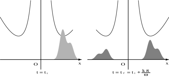
Figure 5: Process of quantum copy through the caustics anomaly. At every period $T=k\pi/\omega$, a mirror image of the original profile on $x>0$ emerges on the other side $x<0$. The relative size of the mirror image depends on $a$ and $k$.

The remarkable point is that, at the periods of oscillation $T=k\pi/\omega$, the amplitude turns out to be

$$K({x_{f}},{t_{f}};{x_{i}},{t_{i}})=(-1)^{k}\cos(ak\pi)\delta({x_{f}}-{x_{i}})+i(-1)^{k}\sin(ak\pi)\delta({x_{f}}+{x_{i}}).$$ (42)

The first term on the r.h.s. corresponds to the return of the particle to its initial position (which is the classical caustics), while the second term corresponds to the tunneling of the particle which reaches the mirror point of the initial position with respect to the singular wall. This shows that the classical caustics has been modified at the quantum level (i.e., caustics anomaly), in such a way that we can now have the mirror image of the original profile prepared at the initial time $t=t_{i}$, with the weight factors being the functions of the parameter $a$ determined from the coupling constant $g$ (and the characteristic matrix $U$ for the general case). In other words, one can ‘copy’ an original profile prepared on the $x>0$ side to the other $x<0$ side after the periods, and that this can be done with desirable weight factors if one can control the relevant parameters of the factors freely [13]. Note that this copying process is not in conflict with the no-go theorem [14] of quantum cloning, because the process takes place in one Hilbert space rather than two as presumed in the theorem.

6 Quantum Force on a Partition Wall

Let us finish our discussion with another example to exhibit how remarkably distinct physics arises for distinct possible dots and walls.

Consider an interval $[-l,l]$ bordered by Dirichlet reflecting walls, $\psi(\pm l)=0$. Suppose we insert a separating dot at the centre with $L(\theta_{+})=\infty$, $L(\theta_{-})=0$, in other words, a partition wall that imposes the Neumann condition from the right and the Dirichlet one from the left. Suppose also that we put $N$ identical bosonic particles into each of the two half wells, which we keep at the same temperature, and calculate the quantum statistical average forces (or pressure) acting on the partition from the right and the left. Notably, the only difference between the circumstances on the two half wells is the distinct reflecting property of the separating wall from the two directions. We will see that, due solely to this fact, the net force will be nonvanishing and reaching arbitrarily large values at high enough temperatures [15].

To see this, we recall first that the right and left half wells admit the energy levels $E^{\pm}_{n}=e^{\pm}_{n}{\cal E}$, $n=1$, $2$, $3$ $\ldots$, with

$$e^{+}_{n}=\left(n-{1\over 2}\right)^{2},\qquad e^{-}_{n}=n^{2},\qquad{\cal E}={{\hbar^{2}}\over{2m}}\left({{\pi}\over{l}}\right)^{2},$$ (43)

where we use hereafter the indices ‘$+$’ and ‘$-$’ to indicate quantities for the right and left half wells, respectively. The particles will distribute among these eigenstates according to the Bose-Einstein statistics,

$$N_{n}^{\pm}={1\over{e^{\alpha^{\pm}+e^{\pm}_{n}/t}-1}},$$ (44)

where $t$ is the dimensionless temperature parameter $t=kT/{\cal E}$, and the temperature dependent $\alpha^{\pm}=\alpha^{\pm}(t)$ are determined by $N=\sum_{n}N_{n}^{\pm}$. The forces acting from the right and the left are given by

$$F^{\pm}=-\sum_{n}{{\partial E_{n}^{\pm}}\over{\partial l}}N_{n}^{\pm}=\frac{2{\cal E}}{l}\sum_{n}e^{\pm}_{n}N^{\pm}_{n}.$$ (45)

For low temperatures, most of the particles are in the ground state, and $N^{\pm}_{n}$ decrease exponentially fast for higher $n$. Consequently, the net force will be contributed essentially by the ground and first excited levels (see Figure 6), giving

$$\Delta F(t)\approx\frac{2{\cal E}}{l}\left[\frac{3}{4}N+3\,e^{-3/t}-2\,e^{-2/t}\right]$$ (46)

Figure 6: The dimensionless net force $\frac{l}{2{\cal E}}\Delta F(t)$ for $N=100$, in the temperature region $t<1$, obtained by a numerical computation (solid line), and approximated by (46) (dashed line).

As temperature is increased, more and more levels enter, and the net force starts to decrease approximately linearly. This behavior can be accounted for by using a heuristic argument [15] which classifies the energy levels into three classes and estimates the contribution of each class in turn. The result,

$$\Delta F(t)\approx\frac{2{\cal E}}{l}\left[{3\over 4}N-{t\over{(e-1)^{2}}}\right]$$ (47)

proves to be satisfactory up to $t\approx 2N/3$, where the net force reaches a minimum and starts to increase afterwards (see Figure 7).

To explain this minimum and the increase following it with an analytic approximation formula, let us replace the infinite sums (45) and $N=\sum_{n}N_{n}^{\pm}$ with corresponding integrals, which is allowed in this temperature region. Assuming $|\alpha^{\pm}|<1$ as well, one then obtains [15]

$$\Delta F\approx\frac{2{\cal E}}{l}\left[\left(Nt+\frac{35}{96}\sqrt{\pi}t^{3/2}\right)\left(\alpha^{+}-\alpha^{-}\right)+\left(\sqrt{e_{1}^{+}}-\sqrt{e_{1}^{-}}\right)t\right],$$ (48)

where the $\alpha^{\pm}$ are to be determined from

$$N \approx \frac{1}{\alpha^{\pm}+e^{\pm}_{1}/t}+\frac{1/2}{\alpha^{\pm}+e^{\pm}_{2}/t}-\frac{3}{4}-\frac{\sqrt{(2-\alpha^{\pm})t}-\sqrt{e^{\pm}_{2}}}{2}$$ (49)

$$+\sqrt{\frac{t}{|\alpha^{\pm}|}}\left[A\left(\sqrt{\frac{|\alpha^{\pm}|t}{e^{\pm}_{2}}}\right)-A\left(\sqrt{\frac{|\alpha^{\pm}|}{2-\alpha^{\pm}}}\right)\right],$$

with $A$ denoting the arctan function for positive $\alpha^{\pm}$ and the arctanh function for negative $\alpha^{\pm}$. It is not easy to express the solution $\alpha^{\pm}$ of (49) directly via an approximate analytic formula, but by calculating the solution numerically and applying it in (48), one can observe that there indeed occur the minimum of the net force and the increase following it (see Figure 7). We point out that, in the dimensionless unit, both the zero temperature limit $\frac{l}{2{\cal E}}\Delta F(0)=\frac{3}{4}N$ and the temperature $t$ at which the net force takes its minimum are of order $N$.

Figure 7: Left: The dimensionless net force $\frac{l}{2{\cal E}}\Delta F(t)$ for $N=100$, in the temperature region $0<t<160$, obtained by a numerical computation (solid line), and approximated by (47) (dotted line), and by (48) using (49) (dashed line). Right: The dimensionless net force $\frac{l}{2{\cal E}}\Delta F(t)$ for $N=100$, obtained by a numerical computation (solid line), and approximated for high temperatures with (56) (dashed line). The figure is double logarithmic.

When we increase the temperature further, we find that the net force keeps increasing, and actually proves to tend to infinity with a square-root-of-temperature asymptotic behavior (see Figure 7). This temperature dependence can be derived as follows. By expanding $N_{n}^{\pm}$ in terms of $q^{\pm}:=e^{-\alpha^{\pm}}$ as

$$N_{n}^{\pm}=\frac{q^{\pm}e^{-e_{n}^{\pm}/t}}{1-q^{\pm}e^{-e_{n}^{\pm}/t}}=\sum_{k=1}^{\infty}(q^{\pm})^{k}e^{-ke^{\pm}_{n}/t},$$ (50)

we have

$$N=\sum\limits_{n=1}^{\infty}N_{n}^{\pm}=\sum\limits_{k=1}^{\infty}(q^{\pm})^{k}\sum\limits_{n=1}^{\infty}e^{-ke_{n}^{\pm}/t}=\sum\limits_{k=1}^{\infty}(q^{\pm})^{k}\left[-\frac{\sigma^{\pm}}{2}+\frac{1}{2}\sum\limits_{n=-\infty}^{\infty}e^{-ke^{\pm}_{n}/t}\right]$$ (51)

with $\sigma^{+}=0$ and $\sigma^{-}=1$. Applying now the Poisson summation formula,

$$\sum_{n=-\infty}^{\infty}y(n)=\sum_{m=-\infty}^{\infty}\int_{-\infty}^{\infty}ds\,y(s)e^{2\pi ims},$$ (52)

we obtain

$$N=\sum\limits_{k=1}^{\infty}(q^{\pm})^{k}\left[-\frac{\sigma^{\pm}}{2}+\sqrt{\frac{\pi t}{4k}}\sum\limits_{m=-\infty}^{\infty}(\mp 1)^{m}e^{-\frac{\pi^{2}t}{k}m^{2}}\right].$$ (53)

Similarly, for the forces $F^{\pm}$ [see (45)], we find

$$F^{\pm}=\frac{2{\cal E}}{l}\sum\limits_{k=1}^{\infty}(q^{\pm})^{k}\sqrt{\frac{\pi t^{3}}{16k^{3}}}\sum\limits_{m=-\infty}^{\infty}(\mp)^{m}\left(1-\frac{2\pi^{2}t}{k}m^{2}\right)e^{-\frac{\pi^{2}t}{k}m^{2}}.$$ (54)

For the high-temperature asymptotic behavior ($N^{\pm}_{1}\to 0\Rightarrow q^{\pm}\to 0$), it suffices to consider only the first two terms in the sums over $k$ in these sums, and within each term to keep only the $m=0$ term in the sums over $m$ (the $m\neq 0$ terms being exponentially suppressed). Thus, from (53) we get

$$q^{\pm}=2N/(\pi t)^{1/2}+2N(\sigma^{\pm}-\sqrt{2}N)/(\pi t)+{\cal O}(t^{-3/2}),$$ (55)

and, correspondingly, the net force,

$$\Delta F=\frac{{\cal E}N}{l}\left(\frac{t}{\pi}\right)^{1/2}+{\cal O}(t^{0}),$$ (56)

which is the promised square-root-of-temperature asymptotic behavior. We can see in Figure 7 how this asymptotic behavior is reached at high temperatures.

The result that the net force does not tend to zero (nor to a nonzero constant) seems unusual when contrasted to the naive expectation that such quantum effects coming from the distinct boundary conditions should vanish at high temperatures where the classical picture would be available. However, this surprising feature can be understood by the fact that, contrary to most quantum systems, one dimensional wells have such energy spectra that the level spacing is not decreasing but increasing for higher energy levels (which is actually valid not only for boxes with Dirichlet and/or Neumann boundary conditions but for all other wells as well [16]). In other words, quantum wells can be distinguished by their high-temperature behavior, too.

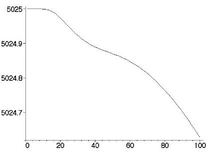
Figure 8: The dimensionless net force $\frac{l}{2{\cal E}}\Delta F(t)$ in the fermionic case, for $N=100$, in the low-temperature region.

One can replace the bosonic particles with fermions, and consider the same problem as above, too. The net force is found to exhibit a qualitatively similar temperature dependence as in the bosonic case, with two main differences. One of them is that the $t=0$ value of the net force and the temperature where the net force takes its minimum are proportional to $N^{2}$ rather than to $N$ as seen in the bosonic case. The other is that one slight “step” can be observed at low temperatures, where the net force starts to decrease from its $t=0$ value (see Figure 8). Otherwise the fermionic case is similar to the bosonic one, and, for example, the high-temperature asymptotics proves to be the same square-root-of-temperature one [17].

7 Discussions

We have discussed in this paper some of the interesting physical phenomena that can arise on a line if there is a controllable point singularity either in the form of a dot or a wall. It is remarkable that putting just a singular point on a line allows for such variety of phenomena — duality, anholonomy, supersymmetry, caustics anomaly and the emergence of pressure — which are found usually in more involved systems such as gauge field theory. In addition, the scale anomaly (i.e. the breakdown of the classical scale symmetry at the quantum level) which we did not mention in this paper can also be seen in the system with a generic singularity. This is implied by the presence of the scale parameters $L(\pm\theta)$, which are missing in the classical description. It is, therefore, safe to say that the crucial element for those quantum phenomena to occur is not in the complexity of the system nor in the infinity of the degrees of freedoms of the system as often assumed. Rather, these are allowed because the quantum description of a system requires more information (and hence more parameters to be fixed) than the classical description does, and that once the extra parameters are chosen, some of the properties that hold classically may no longer hold, causing the anomalies at the quantum level. The extra parameters in the case of a singularity on a line are given by the group $U(2)$, whose global structure is then used to yield the anholonomy effects, for example.

Putting the singularity in many particle systems offers an interesting possibility when considered in the context of statistical mechanics. We have seen this in the simple, albeit not too realistic, example of the quantum force acting on a partition wall in a square potential well. The force attains a minimum at a certain temperature, which is proportional to the particle number $N$ for the bosonic case or to its square $N^{2}$ for the fermionic case, before it diverges for $T\to\infty$. For the bosonic case with $N\sim 100$, the minimum will be seen in a room temperature if the size of the system is about a few hundred nanometers, whereas for the fermionic case the same can be seen even with larger systems of the size of one micron. In view of the rapid progress of nano-technology in recent years, it may not be entirely unreasonable to expect that some of these effects described here can be observed in laboratory in the near future.

References

- [1] M. Reed and B. Simon: Methods of Modern Mathematical Physics II, Fourier analysis, self-adjointness (Academic Press, New York, 1975).
- [2] S. Albeverio, F. Gesztesy, R. Høegh-Krohn and H. Holden: Solvable Models in Quantum Mechanics (Springer, New York, 1988).
- [3] N.I. Akhiezer and I.M. Glazman: Theory of Linear Operators in Hilbert Space, Vol.II (Pitman Advanced Publishing Program, Boston, 1981).
- [4] T. Fülöp and I. Tsutsui: Phys. Lett. A264 (2000) 366.
- [5] I. Tsutsui, T. Cheon and T. Fülöp: J. Phys. A: Math. Gen. 36 (2003) 275.
- [6] I. Tsutsui, T. Fülöp and T. Cheon: J. Phys. Soc. Jpn. 69 (2000) 3473.
- [7] T. Cheon, T. Fülöp and I. Tsutsui: Ann. Phys. 294 (2001) 1.
- [8] I. Tsutsui, T. Fülöp and T. Cheon: J. Math. Phys. 42 (2001) 5687.
- [9] T. Uchino and I. Tsutsui: Nucl. Phys. B662 (2003) 447.
- [10] T. Uchino and I. Tsutsui: J. Phys. A: Math. Gen. 36 (2003) 6821.
- [11] L.S. Schulman: Techniques and Applications of Path Integration (John Wiley and Sons, New York, 1981).
- [12] F. Calogero: J. Math. Phys. 10 (1969) 2191, 2197; 12 (1971) 419.
- [13] H. Miyazaki and I. Tsutsui: Ann. Phys. 299 (2002) 78.
- [14] W.K. Wootters and W.H. Zurek: Nature 299 (1982) 802.
- [15] T. Fülöp, H. Miyazaki and I. Tsutsui: Quantum Force due to Distinct Boundary Conditions, to appear in Mod. Phys. Lett. A; e-print quant-ph/0309095.
- [16] T. Fülöp, I. Tsutsui and T. Cheon: J. Phys. Soc. Jpn. 72 (2003) 2737.
- [17] T. Fülöp and I. Tsutsui: Quantum Force generated by Boundary Conditions, in preparation.