Conditional preparation of a non-classical state in the continuous variable regime: theoretical study

Abstract

We study the characteristics of the quantum state of light produced by a conditional preparation protocol totally performed in the continuous variable regime. It relies on conditional measurements on quantum intensity correlated bright twin beams emitted by a non-degenerate OPO above threshold. Analytical expressions as well as computer simulations of the selected state properties and preparation efficiency are developed and show that a sub-Poissonian state can be produced by this technique. Projection onto a given trigger value is studied and then extended to a finite band. The continuous variable regime offers the unique possibility to improve dramatically the preparation efficiency by choosing multiple selection bands and thus to generate a great number of sub-Poissonian states in parallel.

I Introduction

Conditional state preparation opens the possibility to generate a wide range of non-classical states of light. Quantum correlation between two modes -a signal and a trigger- is the prerequisite for such a general procedure. Pre-assigned events on the trigger condition the readout of the signal and cause a non-unitary state reduction.

Various protocols have been proposed and implemented successfully in the photon counting regime. For instance, this strategy has been widely used to generate single photon Fock state. The required two-mode correlation can be obtained by an atomic cascade Aspect or by the more efficient technique of parametric down conversion fock1 . The single-photon state is created from the initial two-mode state when a photocount event is recorded in the trigger path. Two output ports of a beam splitter can also provide the required correlation: it has been shown theoretically that a squeezed vacuum transmitted through a beam-splitter is reduced to a Schrödinger-cat-like state when a photon is detected on the reflected port dakna . Non classical photon states have also been experimentally prepared by triggering on a given atomic state atom .

Recently, several conditional preparation protocols were introduced for the continuous variable regime where a continuously varying photocurrent is measured instead of single photon counts. For instance in Schiller , continuous measurements are triggered by photocounts. The triggering condition and the characterization of the selected state can also be done both in the continuous variable regime. Some theoretical protocols have been proposed relying on two-mode squeezed vacuum generated by an optical parametric amplifier vacuum .

The scheme we propose relies on quantum intensity correlated bright twin beams -signal and idler- generated by a non-degenerate optical parametric oscillator (ND-OPO) pumped above threshold traditional . The procedure, sketched in Fig. 1, is the following : among all the recorded values of the signal beam intensities, one only keeps the events occurring in the time intervals when the idler intensity takes a given pre-assigned value, or more precisely, lies around this value within a small intensity range. All other time intervals are discarded. In the present paper, we study theoretically this conditional preparation technique. Its experimental implementation and the corresponding results have been detailed in laurat .

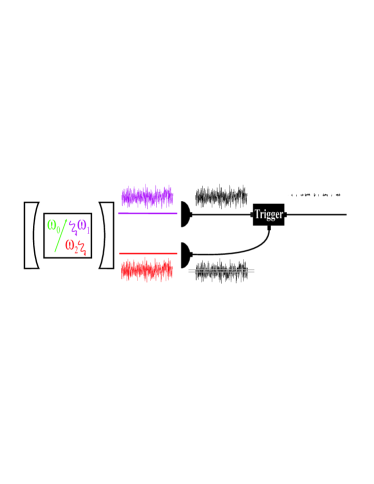
Figure 1: Proposed conditional measurement protocol in the continuous variable regime. A ND-OPO generates above threshold orthogonally polarized and quantum intensity correlated bright twin beams which are detected by high efficiency photodiodes. The continuously varying signal photocurrent is kept only when the idler photocurrent takes a given value or falls inside a narrow band.

This paper is organized as follows. In section II, we describe the quantum state generated by a ND-OPO above threshold. Conditioning on a given value of the idler intensity results in a state reduction which generates a sub-Poissonian state. This procedure, presented in section III, is then extended to the case of a selection interval of bandwidth $\Delta$ around a given value in section IV. The state reduction is characterized according to the initial correlation, individual noise on each beam and position and width of the conditioning band. Section V proposes a Monte-Carlo simulation of the reduced state properties. Section VI is then devoted to multiple-band selection, a possibility to significantly increase the efficiency of the conditional strategy which is only offered by schemes in the continuous variable regime. In section VII, the main conclusions of the paper are summarized and possible extensions to more exotic non-classical states are discussed.

II Quantum state produced by a ND-OPO above threshold

The starting point of the theoretical analysis of the present conditional measurement is the precise knowledge of the quantum state produced by a non-degenerate OPO, from which the conditionally prepared state will be deduced by state reduction. When the twin photons are produced by spontaneous parametric down-conversion, the quantum state of the system is well-known and given by milburn

$$|\Psi\rangle = e^{\left(\lambda\hat{a}_{1}^{+}\hat{a}_{2}^{+}-\lambda^{*}\hat{a}_{1}\hat{a}_{2}\right)}|0,0\rangle$$ (1)

$$= (\cosh\lambda)^{-1}\sum_{n=0}^{\infty}(\tanh\lambda)^{n}|n,n\rangle$$

where the indices 1 and 2 refer respectively to the signal and idler modes and $\hat{a}_{i}$ (resp. $\hat{a}_{i}^{+}$) is the annihilation (resp. creation) operator of a photon in mode $i$. $\lambda$ is proportional to the pump amplitude and crystal non-linearity. The state $|n_{1},n_{2}\rangle$ is a Fock state with $n_{1}$ photons in the signal mode and $n_{2}$ photons in the idler mode. When the parametric down-conversion efficiency is very weak, which is experimentally the most frequent case, the state of the system reduces to the simple entangled state

$$|\Psi\rangle\simeq|0,0\rangle+\lambda|1,1\rangle$$ (2)

When a single photon is detected in the idler mode, the system collapses by the state reduction process into the signal mode single photon state $|1\rangle$, as is well known.

To the best of our knowledge, there is so far no complete theory giving the state of light produced by an OPO in the Schrödinger picture, comparable to the Lamb theory giving the density matrix of the light produced by a laser lamb . The OPO has been described instead in most theoretical approaches in the Heisenberg picture, in terms of operators, which is not useful in the present case. Only Graham et al. graham have considered this problem, mainly to determine the phase diffusion properties of the OPO, and not its joint photon-number distribution.

In the absence of a complete theory, we will use here a semi-phenomenological approach, relying on both theoretical considerations and experimental observations traditional ; laurat : OPOs produce above threshold phase-coherent light in both signal and idler modes which have a Gaussian statistics and present close to threshold a large excess noise compared to the shot noise level. We will call $F$ the Fano factor of this photon distribution defined as the noise variance normalized to the one of a Poissonian distribution of same mean power: close to threshold, this factor is large. Furthermore, one knows that in the absence of losses and in the case of a single output mirror of the OPO cavity, there is a perfect intensity correlation between the two modes when they are measured on time intervals long compared to the cavity storage time reynaud . From this, we infer that the quantum state describing the output of such a perfect OPO is the eigenvector of $\hat{I_{1}}-\hat{I_{2}}=\hat{a}_{1}^{+}\hat{a}_{1}-\hat{a}_{2}^{+}\hat{a}_{2}$ with a zero eigenvalue. By assuming a gaussian photon statistics, the state can be described by

$$|\Psi_{OPO}\rangle=\sum_{n=0}^{+\infty}c_{n}|n,n\rangle$$ (3)

with

$$|c_{n}|^{2}=\frac{1}{\sqrt{2\pi F\bar{n}}}\ \mathrm{exp}\left[-\frac{(n-\bar{n})^{2}}{2F\bar{n}}\right]$$ (4)

or more generally by a density matrix

$$\rho=\sum_{n,n^{\prime}}c_{n,n^{\prime}}|n,n\rangle\langle n^{\prime},n^{\prime}|$$ (5)

with $c_{n,n}$ equal to the expression of $|c_{n}|^{2}$ given by equation (4). This form of the density matrix ensures at the same time a Gaussian distribution of photon numbers in each mode and a perfect intensity correlation between them. It will be shown later that the unknown expressions of $c_{n,n^{\prime}}$ for $n\neq n^{\prime}$ are not relevant in our calculations.

Uncorrelated losses in the system inevitably degrade the initial correlation between the signal and idler modes. These linear losses, that we will assume to be equal for the signal and idler modes, can be modelled by a beam-splitter of intensity reflection coefficient $R$ equal to the loss coefficient and of transmission coefficient $T=1-R$ (Fig. 2). If the input state impinging on such a beam-splitter is the tensor product $|n,0\rangle$ of a Fock state on the input mode 1 and the vacuum in the loss mode, the output state $|\Psi_{out}\rangle$ is loudon

$$|\Psi_{out}\rangle=\sum_{p=0}^{n}A_{n,p}|n-p,p\rangle$$ (6)

with $A_{n,p}$ given by

$$A_{n,p}=\sqrt{\frac{n!}{p!(n-p)!}T^{n-p}R^{p}}$$ (7)

corresponding to a binomial distribution of the photons over the two outputs of the beam-splitter, characteristic of a partition process. The system is then described by a pure state belonging to a four-mode Hilbert space : the signal, idler modes and the two loss modes of the two outputs. By tracing over these two loss modes which are not measured, one obtains the following reduced density matrix

$$\rho^{\prime} = \sum_{n,n^{\prime},p,p^{\prime}}c_{n,n^{\prime}}A_{n,p}A^{*}_{n^{\prime},p}A_{n,p^{\prime}}A^{*}_{n^{\prime},p^{\prime}}$$ (8)

$$\qquad\quad|n-p,n-p^{\prime}\rangle\langle n^{\prime}-p,n^{\prime}-p^{\prime}|$$

This expression is valid for any values of the parameters $R,\bar{n}$ and $F$. From it, one can calculate the probability distribution of the intensity difference. Its mean value is zero. Its variance can be written as

$$\Delta^{2}(\hat{I_{1}}-\hat{I_{2}}) = \mathrm{Tr}(\ \rho^{\prime}(\hat{I_{1}}-\hat{I_{2}})^{2}\ )$$

$$= \sum_{n=0}^{\infty}|c_{n}|^{2}\sum_{p,p^{\prime}=0}^{n}|A_{n,p}|^{2}|A_{n,p^{\prime}}|^{2}(p-p^{\prime})^{2}$$

and becomes

$$\Delta^{2}(\hat{I_{1}}-\hat{I_{2}})=2R\bar{n}T=2R\bar{n}^{\prime}$$ (10)

where $\bar{n}T=\bar{n}^{\prime}$ is the mean photon number of the signal and idler mode after the beam-splitter. $\Delta^{2}(\hat{I_{1}}-\hat{I_{2}})$ is independent of $F$ and coincides with the value obtained by the usual linearized theory for the fluctuations. From this, one finds that the ”gemellity” $G$, which is the remaining noise on the intensity difference normalized to the total shot noise level $2\bar{n}^{\prime}$, is equal to the loss coefficient $R$.

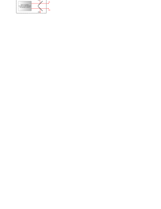
Figure 2: The dotted rectangle models a ND-OPO which can be described by a source of perfect intensity correlated beams plus a partition process generated by two symmetric beam-splitters with intensity transmission $T$ and reflection $R$. The ”gemellity” $G$ of the beams is found to be equal to the loss coefficient $R$.

As bright beams have very large mean values in comparison with the Poissonian standard deviation, one can easily assume that both the reflected and transmitted beams have also large mean values, even for $R$ or $T$ close to 1. Thus, one can use the Stirling’s approximation and show that, in a normalized form

$$|A_{n,p}|^{2}=\frac{1}{\sqrt{2\pi nRT}}\ \mathrm{exp}\left[-\frac{(p-nR)^{2}}{2nRT}\right]$$ (11)

Let us calculate the photon distribution of the individual beams after the beam-splitters. If we only consider measurements involving output 1, the reduced density matrix $\rho^{\prime\prime}$ is obtained by tracing over the output 2

$$\rho^{\prime\prime}=\sum_{n,n^{\prime},p}c_{n,n^{\prime}}A_{n,p}A^{*}_{n^{\prime},p}|n-p\rangle\langle n^{\prime}-p|$$ (12)

The normalized probability distribution for the number of photons can thus be written as

$$P(n_{1}) = \langle n_{1}|\rho^{\prime\prime}|n_{1}\rangle$$

$$= \sum_{n=0}^{+\infty}|c_{n}|^{2}|A_{n,n-n_{1}}|^{2}$$

and becomes

$$\quad P(n_{1}) = \sum_{n=0}^{+\infty}\frac{1}{\sqrt{2\pi F\bar{n}}}\frac{1}{\sqrt{2\pi nRT}}$$

$$\times\mathrm{exp}\left[-\frac{(nT-\bar{n}^{\prime})^{2}}{2F\bar{n}^{\prime}T}-\frac{(n-n_{1}-nR)^{2}}{2nRT}\right]$$

We introduce $\delta=nT-\bar{n}^{\prime}$ and $\varepsilon=n_{1}-\bar{n}^{\prime}$ and we assume that $n$ can be taken constant and equal to $\bar{n}$ in the factor $\frac{1}{\sqrt{2\pi nRT}}$. As the numbers of photon are large, the parameters $\delta$ and $\varepsilon$ can be considered as continuous variables. The sum can thus be rewritten as an integral

$$P(\varepsilon)=\frac{1}{T}\frac{1}{\sqrt{2\pi\bar{n}^{\prime}R}}\frac{1}{\sqrt{2\pi F\bar{n}}}\qquad\qquad\qquad\qquad$$ (15)

$$\int_{-\infty}^{+\infty}\mathrm{exp}\left[-\frac{\delta^{2}}{2F\bar{n}^{\prime}T}\right]\mathrm{exp}\left[-\frac{(\delta-\varepsilon)^{2}}{2R(\delta+\bar{n}^{\prime})}\right]d\delta$$

Developed to the first order in $\frac{\delta}{\bar{n}^{\prime}}$ and $\frac{\varepsilon}{\bar{n}^{\prime}}$

$$\!\!P(\varepsilon)=\frac{1}{T}\frac{1}{\sqrt{2\pi F\bar{n}}}\frac{1}{\sqrt{2\pi\bar{n}^{\prime}R}}\qquad\qquad\quad\qquad\qquad$$ (16)

$$\int_{-\infty}^{+\infty}\!\!\mathrm{exp}\left[-\delta^{2}(\frac{1}{2F\bar{n}^{\prime}T}+\frac{1}{2R\bar{n}^{\prime}})+\delta\frac{\varepsilon}{R\bar{n}^{\prime}}-\frac{\varepsilon^{2}}{2R\bar{n}^{\prime}}\right]d\delta$$

and by using the formula

$$\int_{-\infty}^{+\infty}\mathrm{exp}\left[-A_{1}\delta^{2}+A_{2}\delta\right]d\delta=\sqrt{\frac{\pi}{A_{1}}}\ \mathrm{exp}\left[-\frac{A_{2}^{2}}{4A_{1}}\right]$$ (17)

the probability distribution can be integrated to give

$$P(n_{1})=\frac{1}{\sqrt{2\pi\bar{n}^{\prime}F^{\prime}}}\ \mathrm{exp}\left[-\frac{(n_{1}-\bar{n}^{\prime})^{2}}{2\bar{n}^{\prime}F^{\prime}}\right]$$ (18)

with

$$F^{\prime}=R+FT$$ (19)

Thus we find that the new Fano factor $F^{\prime}$ after the beam-splitter is given by $R+FT$. In the case of important losses ($R\rightarrow 1$, $T\rightarrow 0$), this Fano factor goes to 1, i.e. the output state distribution is Poissonian as expected.

III State reduction by a photon number measurement

In this section, we study the reduced state resulting from a photon number measurement on beam 2 giving the pre-assigned value $N$. By tracing over the trigger mode, the reduced density matrix $\rho^{\prime\prime\prime}$ for the signal mode only can be written as

$$\rho^{\prime\prime\prime}=\sum_{n,n^{\prime},p}c_{n,n^{\prime}}A_{n,p}A^{*}_{n^{\prime},p}A_{n,n-N}A^{*}_{n^{\prime},n-N}$$

$$\qquad\quad|n-p\rangle\langle n^{\prime}-p|$$ (20)

One can see that the photon probability distribution depends only on the diagonal terms of the density matrix $\rho$. The photon probability distribution of beam 1 when a given value $N$ is measured on beam 2 is thus

$$P(n_{1},n_{2}=N)=\sum_{n=0}^{+\infty}|c_{n}|^{2}|A_{n,n-n_{1}}|^{2}|A_{n,n-N}|^{2}$$ (21)

With $F^{\prime}$ and $\bar{n}^{\prime}$ the Fano factor and mean value established in the last section, this distribution can be read as

$$P(n_{1},N) = \frac{1}{\sqrt{2\pi F\bar{n}}}\sum_{n=0}^{+\infty}\frac{1}{2\pi nRT}\ \mathrm{exp}\left[-\frac{(nT-\bar{n}^{\prime})^{2}}{2(F^{\prime}-R)\bar{n}^{\prime}}\right.$$ (22)

$$\left.-\frac{(nT-n_{1})^{2}}{2nRT}-\frac{(nT-N)^{2}}{2nRT}\right]$$

Let us consider $\varepsilon=n_{1}-\bar{n}^{\prime}$ introduced in the previous section and $\alpha=N-\bar{n}^{\prime}$ which corresponds to the distance between the value of conditioning $N$ and the distribution center $\bar{n}^{\prime}$. Using calculation techniques similar to the ones of the previous section, the probability distribution can finally be written as

$$P(\varepsilon,\alpha) = \left(\frac{1}{\sqrt{2\pi\bar{n}^{\prime}F^{\prime}}}\ \mathrm{exp}\left[-\frac{\alpha^{2}}{2\bar{n}^{\prime}F^{\prime}}\right]\right)$$ (23)

$$\times\left(\frac{1}{\sqrt{2\pi\bar{n}^{\prime}V_{c}}}\ \mathrm{exp}\left[-\frac{(\varepsilon-\beta\alpha)^{2}}{2\bar{n}^{\prime}V_{c}}\right]\right)$$

with

$$\beta=1-\frac{G}{F^{\prime}}$$ (24)

$$V_{c}=2G-\frac{G^{2}}{F^{\prime}}$$ (25)

$V_{c}$ is the conditional variance of the intensity fluctuations the signal beam knowing the intensity fluctuations of the trigger beam. This parameter plays an important role in the characterization of Quantum Non Demolition measurements qnd .

The first factor between parenthesis in equation (23) expresses the preparation probability, i.e. the proportion of selected points in an experimental implementation. It is maximum when $\alpha=0$. A value chosen in the wings of the gaussian distribution leads to a smaller efficiency. The preparation probability is inversely proportional to $\sqrt{F^{\prime}\bar{n}^{\prime}}$. This factor is thus very small in the case of bright beams: for 1064 nm beams with a mean power of 1 mW and a Fano factor equal to 100, the maximal preparation probability obtained when $\alpha=0$ is as small as $5.10^{-10}$.

The second factor of this probability shows that the selected state has a gaussian photon distribution centered around the value $\beta\alpha$, slightly different from the triggering value $\alpha$ except for $\alpha=0$. This difference can be interpreted by the dissymmetry of the probability distribution around the conditioning value. For a conditioning value equal to the mean of the distribution ($\alpha=0$), this difference vanishes as the distribution is symmetric.

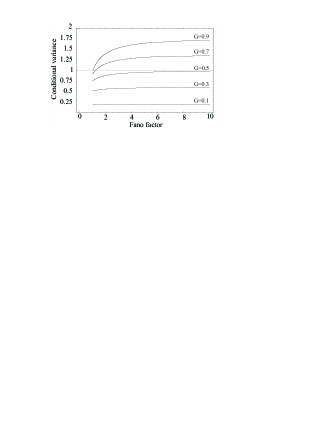
Figure 3: Conditional variance as a function of the Fano factor for different initial intensity correlation between signal and idler beams, measured by the ”gemellity” $G$. Values of $G$ as small as $0.1$ have been obtained experimentally laurat2 .

According to (23), the reduced state has a photon variance equal to the conditional variance $V_{c}$. This shows that the selection process we have used in the conditional measurement has extracted the maximum information available from the correlation of the two beams and has transferred it to the signal beam. This beam can exhibit a sub-Poissonian photon distribution when $V_{c}<1$. Figure (3) shows the conditional variance as a function of the Fano factor for different gemellities $G$. If the correlation is perfect, this protocol generates a number state. It is worth noting that for a gemellity inferior to 0.5 the distribution is sub-Poissonian whatever the initial Fano factor. For large Fano factors, which is the experimental case, the noise reduction is twice the initial gemellity as $V_{c}$ can be approximated by $2G$.

The conditional variance $V_{c}$ also characterizes the noise reduction obtained when an active feed-forward correction of signal beam intensity is implemented by opto-electronics devices controlled by information collected on the idler mertz . The two techniques which take advantage of the quantum correlation have therefore the same ultimate performance.

IV State reduction by a band selection

As shown in the previous section, triggering on a single value of photon number in our regime of bright beams where $\bar{n}^{\prime}$ is very large leads to a close to zero preparation probability incompatible with experimental implementation. An interesting question is to determine the photon distribution when one projects onto a finite band instead of a given value. It is worth pointing out that it is always the experimental case because of the limited acquisition precision.

Let us consider a conditioning band of width $\Delta$ around the value $N=\bar{n}^{\prime}+\alpha$. The photon probability distribution of the reduced state can now be written

$$P\left(\varepsilon,\alpha\!-\!\frac{\Delta}{2}\!<\!n_{2}-\bar{n}^{\prime}\!<\!\alpha\!+\!\frac{\Delta}{2}\!\right)=\frac{1}{\sqrt{2\pi\bar{n}^{\prime}F}}\frac{1}{\sqrt{2\pi\bar{n}^{\prime}V_{c}}}$$

$$\int^{\alpha+\frac{\Delta}{2}}_{\alpha-\frac{\Delta}{2}}\mathrm{exp}\left[-\frac{x^{2}}{2\bar{n}^{\prime}F^{\prime}}\right]\mathrm{exp}\left[-\frac{(\varepsilon-\beta x)^{2}}{2\bar{n}^{\prime}V_{c}}\right]dx\qquad$$ (26)

and integrated as

$$P\left(\varepsilon,\alpha\!-\!\frac{\Delta}{2}\!<\!n_{2}-\bar{n}^{\prime}\!<\!\alpha\!+\!\frac{\Delta}{2}\!\right)=\qquad\qquad\qquad\qquad$$

$$\frac{1}{\sqrt{2\pi F^{\prime}\bar{n}^{\prime}}}\ \mathrm{exp}\left[-\frac{\varepsilon^{2}}{2\bar{n}^{\prime}F^{\prime}}\right]\qquad\qquad$$

$$\times\frac{1}{2}\left(\mathrm{erf}\left[\frac{(\alpha+\frac{\Delta}{2})-\beta\varepsilon}{\sqrt{2\bar{n}^{\prime}V_{c}}}\right]-\mathrm{erf}\left[\frac{(\alpha-\frac{\Delta}{2})-\beta\varepsilon}{\sqrt{2\bar{n}^{\prime}V_{c}}}\right]\right)\quad$$ (27)

where erf denotes the error function.

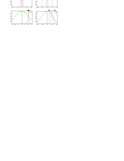
Figure 4: Photon probability distributions of conditionally prepared state. The probability distributions are all normalized to 1 at their maximums for clarity of the plots. The horizontal unit is the width $\sigma=\sqrt{\bar{n}^{\prime}}$ of the Poisson distribution of same mean intensity. Thick curves give the initial gaussian distribution and dashed ones correspond to a coherent state of same mean intensity. Arrows give the extension of the selection band. (a) and (b): the selection band is centered on the mean value ($\alpha=0$). The bandwidth is $\Delta=0.1\sigma$ for (a) and $10\sigma$ for (b). A large band results in a wide distribution (Kurtosis coefficient lower than 3). (c) and (d): the band is centered on $\alpha=10\sigma$. $\Delta=0.1\sigma$ for (c) and $10\sigma$ for (d). Non central selection band results in an asymmetry of the distribution (non null skewness) ($F^{\prime}=100,G=0.18$)

From this exact expression, one can plot the probability distribution of the conditionally prepared state in different cases. The initial Fano Factor and gemellity are taken from our ND-OPO experiment detailed in laurat ($F^{\prime}=100,G=0.18$). Figure (4) gives the photon probability distribution in different possible configurations. The band can be centered around the mean ($\alpha=0$) or around an arbitrary value taken in the wings of the initial gaussian distribution ($\alpha\neq 0$). The bandwidth $\Delta$ can also be small or large relative to the standard deviation $\sigma$ of a Poisson distribution of same mean intensity. The noise distribution of the initial state and of a coherent state of same mean intensity have been superimposed. One observes a narrowing of the probability distribution below the shot noise level in the case of a very narrow bandwidth for any band center. When the bandwidth increases, the reduced state differs more and more from a gaussian distribution.

The distance from a gaussian distribution can be characterized by the coefficients of skewness and kurtosis which are related to higher moments of the probability distribution mandel . The coefficient of skewness provides a dimensionless measure of the asymmetry of the probability distribution. Skewness is null when the band is centered on the mean value. For a normalized probability total surface, the kurtosis coefficient distinguishes distribution which are tall and thin from those that are short and wide. It has the value of 3 for a gaussian distribution and a value lower than 3 corresponds to a less peaked distribution. Let us note that the third order cumulant corresponds to the kurtosis excess. A very small value of kurtosis is associated to a square-shaped distribution. A perfect gaussian distribution is obtained in the limit of very narrow bandwidth -as calculated in the previous section- or in the case of very large bandwidth which corresponds to keep all the values and the selected state corresponds thus to the initial state. A narrow band of selection results in a close to gaussian distribution with a kurtosis coefficient almost constant around 3. This coefficient decreases when the band is extended (Fig. 5).

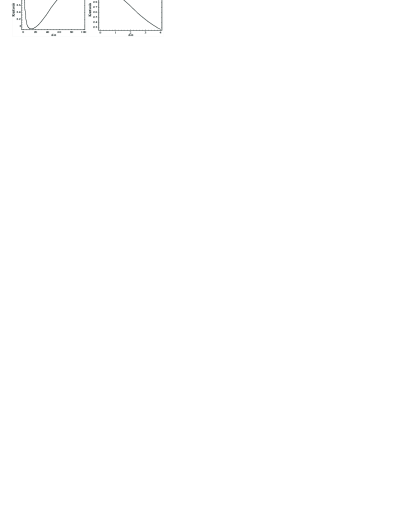
Figure 5: Kurtosis coefficient of the conditionally selected state according to the selection bandwidth normalized to $\sigma=\sqrt{\bar{n}^{\prime}}$ (b): zoom for small bandwidth. ($\alpha=0,F^{\prime}=100,G=0.18$)

We can derive from equation (IV) an approximate but analytical expression for the probability distribution by expanding in powers of $\frac{\Delta}{\sqrt{\bar{n}^{\prime}}}$

$$P\left(\varepsilon,\alpha\!-\!\frac{\Delta}{2}\!<\!n_{2}-\bar{n}^{\prime}\!<\!\alpha\!+\!\frac{\Delta}{2}\!\right)=P(\varepsilon,\alpha)\qquad\qquad\quad$$ (28)

$$\times\left(\!\Delta+\frac{\Delta^{3}}{24\bar{n}^{\prime}V_{c}^{2}}(-1+\frac{(\alpha-\beta\varepsilon)^{2})}{\bar{n}^{\prime}V_{c}}+o\left(\!\left(\frac{\Delta}{\sqrt{\bar{n}^{\prime}}}\!\right)^{5}\right)\!\right)$$

with $P(\varepsilon,\alpha)$ the probability distribution determined in the last section.

Let us underline that for $\Delta=1$ the photon distribution is equal to the one established in the last section. This value corresponds to the minimum bandwidth necessary to discriminate two consecutive photon-number states.

The third order term in $\Delta$ can be neglected in this approximation as long as $\Delta\ll\sigma=\sqrt{\bar{n}^{\prime}}$. The preparation probability can then be written

$$\frac{N_{selected}}{N_{total}}=\frac{(\Delta/\sigma)}{\sqrt{2\pi F^{\prime}}}\ \mathrm{exp}\left[-\frac{(\alpha/\sigma)^{2}}{2F^{\prime}}\right]$$ (29)

where $N_{total}$ and $N_{selected}$ correspond respectively to the total number of events and to the number of selected ones by the conditional protocol.

As a result, conditioning on a narrow band results in a preparation probability proportional to $\Delta$ without decreasing the non classical character of the projected state. This range of $\Delta$ is the optimal one in order to generate a sub-Poissonian state. With a bandwidth equal to $0.1\sigma$ the efficiency reaches $0.4\%$.

From equation (IV), it is possible to compute the exact properties of the state for any value of $\Delta$. In Fig. (6), we give the noise reduction and the probability of preparation for a narrow bandwidth. One can see that for very narrow bandwidth the preparation efficiency increases linearly with the bandwidth whereas the squeezing is almost constant. This corresponds to the first order in $\Delta$ as appears in (28). For a larger band, the efficiency still increases but at the expense of a decreased noise reduction. The efficiency would be higher for an initial state with less excess noise above shot noise. This case can correspond to a ND-OPO pumped well above threshold where it has been shown theoretically that both twin beams can be individually squeezed individual and still highly correlated. In the case of narrow bandwidth, the band center has no effect on the non classical character but results in a lowered preparation efficiency due to the gaussian distribution of the initial noise (Fig. (7)). It is worth noting that the large extension of the initial noise should permit to implement a great number of independent selection bands. Section VI is devoted to this particular conditional strategy offered by continuous variable regime.

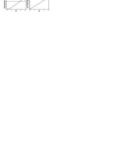
Figure 6: (a) Intensity noise on the reduced state and (b) preparation probability (proportion of selected points) as a function of the selection bandwidth normalized to $\sigma$. ($\alpha=0,F^{\prime}=100,G=0.18$)

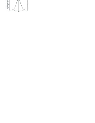
Figure 7: Preparation probability as a function of the center of the narrow $\Delta=0.1\sigma$ selection band. ($F^{\prime}=100,G=0.18$)

V Monte-Carlo simulation of the state reduction

So far we have examined the conditionally prepared state from its theoretical probability distribution expression. However, our protocol is easy to test by Monte-Carlo simulations.

In order to implement the protocol, one needs to prepare two random arrays $A$ and $B$ with super-Poissonian statistics and exhibiting a given amount of correlations. These two arrays will correspond to the fluctuation distribution of the signal and idler twin beams. Actually, we generate three independent arrays. Let us call $C$ a super-Poissonian distribution and $X$ and $Y$ two Poissonian distributions. If the correlation between the signal and idler beams is perfect, we associate to the signal and idler beams the same distribution $C$. For a finite amount of correlations, a similar strategy to the one detailed in section II is performed. We add to the initial common distribution $C$ independent contributions which can be seen as vacuum contributions when the initial state is incident on a beam splitter with reflection coefficient $R$. The statistics distribution of signal and idler after the partition process can be defined by

$$A=\sqrt{R}~{}X+\sqrt{1-R}~{}C$$

$$B=\sqrt{R}~{}Y+\sqrt{1-R}~{}C$$ (30)

The parameter $R$ is the same as the one used in previous sections and determines the gemellity of the beams.

The selection of relevant events can then be done. It is worth noting that conditional measurement experiments are very frequently made after the end of the physical measurement, i.e. by post-selection of the events laurat . So, when the two previous distributions have been generated, we dispose of the same kind of data that after an experiment.

We have simulated all the properties presented before. As expected, the simulations are in perfect agreement with our theoretical predictions. Such simulations also should allow to test the protocol when $\bar{n}^{\prime}$ is not too large, a case where the approximations leading to equation (23) are no longer valid.

VI Multi-band selection

In any conditional protocol, the preparation probability in a given time interval is an important parameter to characterize its efficiency. The efficiency of all conditional preparation techniques is usually very low. Improving the brightness of the source is thus an important and topical challenge in the photon counting regime brightness . The preparation probability is also low in our protocol as shown in Fig. (6) and (7) but the continuous detection results in a great number of selected points in a very short recording time laurat .

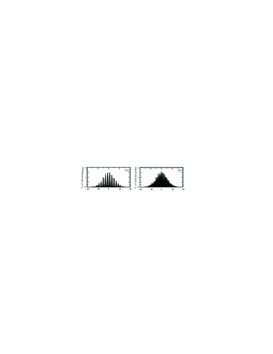
Figure 8: Experimental multi-band selection. The horizontal unit is the width $\sigma$ of the Poisson distribution of same mean intensity. Independent bands of width $\Delta=0.2\sigma$ have been implemented. Band are separated by $4\sigma$ in (a) and $2\sigma$ in (b). ($F^{\prime}=100$, $G=0.18$)

Furthermore, the continuous variable regime offers the possibility to improve the efficiency of the conditional measurement strategy by a large factor. This possibility does not exist for the single photon counting case. One can implement multiple selection bands with different centers on the idler intensity. Independent selection bands will correspond to independent sets of time windows. In each of them, the state is reduced to a given sub-Poissonian state with a constant noise reduction, wherever the band center. By using independent intervals, one keeps most of the values of the idler intensity and so improve by a large factor the success rate of the preparation. This scheme -directly related to the nature of continuous variable- opens the possibility to generate in parallel a great number of sub-Poissonian states. Figure (8) gives the experimental implementation of multi-band selection for different distances between the band center. Experimental details are given in laurat .

VII Conclusions

In the photon counting regime, conditional measurements plays a crucial role as illustrated by the various schemes theoretically proposed or experimentally implemented. The extension to the continuous variable regime is of great importance as the efficiency can be dramatically improved and more complex triggering schemes implemented.

The required quantum correlation is generated in our protocol by a ND-OPO above threshold. It has been shown that conditioning on a given value of the idler intensity leads to the preparation of a sub-Poissonian state with a noise reduction equal to the conditional variance, i.e. the initial gemellity minus 3 dB in the case of a large Fano factor. We have extended this triggering condition to a finite band. For a band largely narrower than the standard deviation of a coherent state of same mean intensity, the preparation probability increases linearly with the bandwidth and the noise reduction remains almost constant. As opposed to the discrete variables case, there is a trade-off between the preparation efficiency and the non classical character of the selected state. Theoretical calculations and computer simulations are in very good agreement, and both account very well for the experimental results detailed in laurat .

The next step should be to extend this conditional measurement strategy to the preparation of more exotic non-classical states as it is the case in the photon counting regime. One can think for instance to generate Schrödinger-cat-like state. It could be also of great interest to extend this protocol to EPR beams, in particular generated by a self-phase-locked OPO where the anti-correlated phase fluctuations of the twin beams are accessible longchambon .

- (1) P. Grangier, G. Roger, A. Aspect, Europhys. Letters 1,173 (1986).
- (2) C.K. Hong, L. Mandel, Phys. Rev. Lett. 56, 58 (1986).
- (3) M. Dakna, T. Anhut, T. Opatrny, L. Knöll, D.G. Welsch, Phys. Rev. A 55, 3184 (1997).
- (4) J.-M. Raimond, M. Brune, S. Haroche, Rev. Mod. Phys. 73, 565 (2001).
- (5) G.T. Foster, L.A. Orozco, H.M. Castro-Beltran, H.J. Carmichael, Phys. Rev. Lett. 85, 3149 (2000); A.I. Lvovsky, H. Hansen, T. Aichele, O. Benson, J. Mlynek, S. Schiller, Phys. Rev. Lett. 87, 050402 (2001)
- (6) K. Watanabe, Y. Yamamoto, Phys. Rev. A 38, 3556 (1988); J. Fiurásek, Phys. Rev. A 64, 053817 (2001); G.M. D’Ariano, P. Kumar, C. Macchiavello, L. Maccone, N. Sterpi, Phys. Rev. Lett. 83, 2490 (1999).
- (7) A. Heidmann, R.J. Horowicz, S. Reynaud, E. Giacobino, C. Fabre, G. Camy, Phys. Rev. Lett. 59, 2555 (1987); J. Mertz, T. Debuisschert, A. Heidmann, C. Fabre, E. Giacobino, Opt. Lett. 16, 1234 (1991); J. Gao, F. Cui, C. Xue, C. Xie, K. Peng, Opt. Lett. 23, 870 (1998).
- (8) J. Laurat, T. Coudreau, N. Treps, A. Maître, C. Fabre, Phys. Rev. Lett. 91, 213601 (2003)
- (9) D.F. Walls, G.J. Milburn, Quantum Optics (Springer-Verlag, First published 1994)
- (10) M. Sargent, M.O. Scully, W.E. Lamb, Laser Physics (Addison-Wesley Publishing Company, First published 1974)
- (11) R. Graham, H. Haken, Z. Physik 210, 276 (1968); R. Graham, Z. Physik 210, 319 (1968); R. Graham, Z. Physik 210, 469 (1968).
- (12) S. Reynaud, C. Fabre, E. Giacobino, J. Opt. Soc. Am. B 4, 1520 (1987)
- (13) R. Loudon, The quantum theory of light (Oxford University Press, Oxford, First published 1973)
- (14) P. Grangier, J.-M Courty, S. Reynaud, Opt. Commun. 83, 251 (1991); J.-Ph Poizat, J.F. Roch, P. Grangier, Ann. Phys. Fr. 19, 265 (1994).
- (15) J. Laurat, L. Longchambon, T. Coudreau, C. Fabre, unpublished result (2002).
- (16) J. Mertz et al., Phys. Rev. Lett. 64, 2897 (1990); J. Mertz, A. Heidmann, C. Fabre, Phys. Rev. A 44, 3229 (1991)
- (17) L. Mandel, E. Wolf, Optical coherence and quantum optics (Cambridge University Press, First published 1995)
- (18) C. Fabre, E. Giacobino, A. Heidmann, S. Reynaud, J. Phys. 50, 1209 (1989); A. Porzio, F. Sciarrino, A. Chiummo, M. Fiorentino and S. Solimeno, Optics Comm. 194, 373 (2001);
- (19) P. G. Kwiat, E. Waks, A. G. White, I. Appelbaum, and P. H. Eberhard, Phys. Rev. A 60, 773 (1999)
- (20) L. Longchambon, J. Laurat, T. Coudreau, C. Fabre, submitted to Eur. Phys. Journ. D, quant-ph/0310036; L. Longchambon, J. Laurat, T. Coudreau, C. Fabre, submitted to Eur. Phys. Journ. D, quant-ph/0311123