Phase dynamics of a multimode Bose condensate controlled by decay

Abstract

The relative phase between two uncoupled BE condensates tends to attain a specific value when the phase is measured. This can be done by observing their decay products in interference. We discuss exactly solvable models for this process in cases where competing observation channels drive the phases to different sets of values. We treat the case of two modes which both emit into the input ports of two beam splitters, and of a linear or circular chain of modes. In these latter cases, the transitivity of relative phase becomes an issue.

I Introduction

Since the first observation of Bose-Einstein condensation, the formation and the nature of the relative phase between two condensates has been a central issue of many theoretical and experimental studies. It has been predicted by Javanainen and Yoo [1] and observed by Andrews et al [2] that two interfering Bose condensates exhibit a clear spatial interference pattern. This shows that in a single run of an interference experiment, they manifest themselves as being coherent. Furthermore, it was predicted in [1] that two cases should be distinguished. When a cold cloud of atoms is first split into two modes, which are separately cooled further into two condensates ( ”cut - then- cool”), two independent condensates arise. Alternatively, two correlated condensates arise when a single condensate is split into two parts (” cool - then - cut”) [2, 3]. Interference pattern from two independent condensates can be different for each realization of interference experiment, while correlated condensates show the same interference pattern for each run. Cirac et al [4] showed by analytical arguments that a system consisting of two independent Bose condensates evolves into a state with a fixed relative phase if one detects the emitted bosonic atoms while observing their spatial interference pattern.

A number of authors have studied the possible manipulation of phase coherence and entanglement between two or more Bose condensates, with tunneling interaction as the key mechanism [5, 6, 7]. A scheme has been proposed to use an interferometric scheme including an atomic beam splitter to recombine two modes in order to reconstruct the state of a two-mode condensate [8]. The buildup of a relative phase between two independent condensates has also been investigated in the situation that the atoms emitted from the two condensates are mixed in a 50:50 beam splitter[9, 10]. Two initially independent bosonic modes, described by a factorized state, evolve into an entangled state of the two modes after a large number of detections in the output ports of the beam splitter. The relative phase distribution shows two narrow peaks, at positions determined by the settings of the beam splitter. The most probable detection history has the form of bosons bunching into a single output channel. An exactly solvable analytical model has been discussed [10], which allows one to get closed expression for the particle detection statistics over two output channels of the beam splitter for a fixed total number of detections. It is remarkable that even though both detection channels are identical, in the most probable history all particles are detected in the same port. This is obviously connected to the bosonic nature of the particles, for which boson accumulation applies. This can likewise be interpreted as a spontaneous selection of a single relative phase. When the first particle chooses randomly one of the two output ports, the following particles have a tendency to choose the same port, and the relative phase of the modes converges to one of the phases imposed by the beam splitter. This can also be viewed as an example of spontaneous symmetry breaking [11]. The role of interparticle interaction is also discussed, and it has been shown that it leads to collapse and revival of the relative phase distribution, thereby reflecting the discrete nature of the states of the system[9].

In the presence of a single beam splitter, the relative phase converges eventually to a single value. It is interesting to consider cases where more detection channels are present which tend to project the relative phase on different values, so that a detection from one beam splitter favors phase values that are incompatible with the setting of another one. In the present paper we consider a number of model cases where such a conflicting tendency arises. This raises the question whether in the end the system simply settles down in one of the possible phase values, or whether it continues to shift between values, without ever coming to a final decision. We consider cases where the detection statistics can be solved analytically. Also we study the effect of a direct Hamiltonian coupling between the condensates on both the detection statistics and the corresponding behavior of the relative phase. Examples of such couplings are tunneling between condensates in two spatially separated potential wells, or stimulated Raman coupling between two condensates corresponding to two different internal states [12]. We treat the condensates just as modes of bosonic particles, so that most of the considerations hold just as well for photons in cavities.

II Quantum states of two boson modes

It will be convenient to express the states of two boson modes in terms of spin-coherent states (SCS), which is normally defined for the $2J+1$-dimensional manifold of states with angular momentum $J$ [13]. The spin-coherent state $\left|\theta,\phi\right\rangle$ is the eigenstate of the component $\overrightarrow{u}\cdot\widehat{\overrightarrow{J}}$ of the angular momentum vector with the maximal eigenvalue $J$, where $\overrightarrow{u}\equiv\widehat{x}\cos\phi\sin\theta+\widehat{y}\sin\phi\sin\theta+\widehat{z}\cos\theta$ is the unit vector in the direction specified by the spherical angles $\theta$ and $\phi$. This state is obtained from the eigenstate of $J_{z}$ with eigenvalue $J$ after performing the appropriate rotation. In the context of two boson modes (or two harmonic oscillators), an $SU(2)$ representation arises by introducing the fictitious angular-momentum operators

$$\widehat{J}_{x}={\frac{1}{2}}\left(\widehat{a}^{\dagger}\widehat{b}+\widehat{b}^{\dagger}\widehat{a}\right),\;\widehat{J}_{y}=\frac{1}{2i}\left(\widehat{a}^{\dagger}\widehat{b}-\widehat{b}^{\dagger}\widehat{a}\right),\widehat{J}_{z}={\frac{1}{2}}\left(\widehat{a}^{\dagger}\widehat{a}-\widehat{b}^{\dagger}\widehat{b}\right),$$ (1)

where $\widehat{a}$ and $\widehat{b}$ are the annihilation operators for modes $A$ and $B$. This is the well-known Schwinger representation. These operators obey the standard commutation rules of angular momentum ($[\widehat{J}_{x},\widehat{J}_{y}]=i\widehat{J}_{z}$, etc.), so that the matrix form of the operators (1) on the eigenvectors of $\widehat{J}_{z}$ and $\widehat{\overrightarrow{J}}^{2}$ attains the shape that is well-known from angular-momentum algebra. Notice that $\widehat{\overrightarrow{J}}^{2}=\frac{\widehat{N}}{2}(\frac{\widehat{N}}{2}+1)$, with $\widehat{N}=\widehat{a}^{\dagger}\widehat{a}+\widehat{b}^{\dagger}\widehat{b}$ the number operator. The eigenvectors of $\widehat{J}_{z}$ and $\widehat{\overrightarrow{J}}^{2}$are just the double Fock states $\left|n_{a},n_{b}\right\rangle$. A given number of particles $N$ corresponds to the value $J=N/2$. The eigenstate of $\widehat{J}_{z}$ with this same eigenvalue is the Fock state $\left|N,0\right\rangle$, so that the SCS with direction $\overrightarrow{u}$can be defined by the rotation

$$\left|\theta,\phi\right\rangle_{N}=\widehat{R}(\theta,\phi)\left|N,0\right\rangle,$$ (2)

with the rotation operator

$$\widehat{R}(\theta,\phi)=\exp(-i\phi\widehat{J}_{z})\exp(-i\theta\widehat{J}_{y})\exp(i\phi\widehat{J}_{z})=\exp[-i\theta(\widehat{J}_{y}\cos\phi-\widehat{J}_{x}\sin\phi)].$$ (3)

The SCS can be represented as a point on a sphere of radius $J$, specified by the polar angle $\theta$, and the azimuthal angle $\phi$. This sphere generalizes the Bloch sphere, describing the state of a spin $1/2$, or the Poincaré sphere which describes the polarization state of a light beam or a photon. In the present case, the radius specifies the number of particles $N=2J$. An explicit expansion of the SCS (2) in the Fock states follows then from the transformation of the creation operators

$$\widehat{R}(\theta,\phi)\widehat{a}^{\dagger}\widehat{R}^{\dagger}(\theta,\phi)=\widehat{a}^{\dagger}\cos\frac{\theta}{2}+\widehat{b}^{\dagger}\sin\frac{\theta}{2}e^{i\phi}\equiv\widehat{c}^{\dagger}(\theta,\phi).$$ (4)

The SCS (2) is found after operating $N$ times with the operator $\widehat{c}^{\dagger}(\theta,\phi)$ on the vacuum state, which leads to the explicit result

$$\left|\theta,\phi\right\rangle_{N}=\sum_{n=0}^{N}\left(\begin{array}[]{l}N\\ n\end{array}\right)^{1/2}\cos^{n}\frac{\theta}{2}\text{ }\sin^{N-n}\frac{\theta}{2}\text{ }e^{i\left(N-n\right)\phi}\text{ }\left|n,N-n\right\rangle.$$ (5)

This demonstrates that the SCS $\left|\theta,\phi\right\rangle_{N}$ can be viewed as a number state in the mode that is a linear combination of the modes $A$ and $B$, and for which the operator $\widehat{c}^{\dagger}(\theta,\phi)$, defined in (4), is the creation operator. In the SCS, the distribution of the $N$ particles over the two modes is binomial, and the angle $\theta$ specifies the average partition by $\left\langle n_{a}\right\rangle=N\cos^{2}\frac{\theta}{2}$ and $\left\langle n_{b}\right\rangle=N\sin^{2}\frac{\theta}{2}$. The azimuthal angle $\phi$ represents the relative phase. This quantity is complementary to the number difference $\widehat{a}^{\dagger}\widehat{a}-\widehat{b}^{\dagger}\widehat{b}$. Number states with all particles in the mode $A$ are represented by the North pole of the Bloch sphere ($\theta=0$), while the South pole represents the SCS with all $N$ particles in mode $B$. Points on the equator ($\theta=\pi/2$) stand for states with equal population of the modes. Since the state (2) (or (5)) is eigenstate of $\widehat{N}$, the absolute phase is fully undetermined.

The relation between the SCS and the more common Glauber coherent states (GCS) is easily found by representing the latter ones in the form

$$\left|r_{a}e^{-i\phi_{a}},r_{b}e^{-i\phi_{b}}\right\rangle=e^{-(r_{a}^{2}+r_{b}^{2})/2}\sum_{N}\frac{1}{N!}(r_{a}e^{-i\phi_{a}}\widehat{a}^{\dagger}+r_{b}e^{-i\phi_{b}}\widehat{b}^{\dagger})^{N}\left|vac\right\rangle.$$ (6)

These states are eigenstates of $\widehat{a}$ and $\widehat{b}$, and they are obviously factorized, so that they carry no entanglement between the modes. It is easy to check that they are related to the SCS by the expansion

$$\left|r_{a}e^{-i\phi_{a}},r_{b}e^{-i\phi_{b}}\right\rangle=e^{-R^{2}/2}\sum_{N}\frac{1}{\sqrt{N!}}R^{N}e^{-iN\phi_{a}}\left|\theta,\phi\right\rangle_{N},$$ (7)

with the parameters $R$, $\theta$ and $\phi$ determined by $R^{2}=r_{a}^{2}+r_{b}^{2}$, $\tan\frac{\theta}{2}=r_{b}/r_{a}$, and $\phi=\phi_{a}-\phi_{b}$. This indicates that the GCS has a Poissonian distribution of the total particle number $N$, with average value $\left\langle N\right\rangle=R^{2}$, while the absolute phases $\phi_{a}$ and $\phi_{b}$ of both modes are well-specified. For bosonic atoms, states with different total number of particles do not superpose, according to the superselection rule, so that we have to restrict ourselves to density matrices that are diagonal in $N$. Since the particle number is conjugate to the overall phase, we introduce the density matrix

$$\widehat{\rho}(R,\theta,\phi)=\frac{1}{2\pi}\int_{0}^{2\pi}d\phi_{a}\left|r_{a}e^{-i\phi_{a}},r_{b}e^{-i(\phi_{a}-\phi)}\right\rangle\left\langle r_{a}e^{-i\phi_{a}},r_{b}e^{-i(\phi_{a}-\phi)}\right|$$ (8)

as the uniform mixture of the GCS (6) over the overall phase $\phi_{a}$, for a given value of the relative phase $\phi=\phi_{a}-\phi_{b}$. Applying eq. (7) leads to an expansion of this same density matrix in the SCS, in the form

$$\widehat{\rho}(R,\theta,\phi)=e^{-R^{2}}\sum_{N}\frac{1}{N!}R^{2N}\left|\theta,\phi\right\rangle_{N}{}_{N}\left\langle\theta,\phi\right|.$$ (9)

The density matrix $\widehat{\rho}(R,\theta,\phi)$ is therefore diagonal in the particle number $N$.

We observe that to each pair of spherical angles $\theta$ and $\phi$, or, equivalently, to each real Cartesian unit vector $\overrightarrow{u}$, corresponds a density matrix $\widehat{\rho}(R,\theta,\phi)$, and an annihilation operator $\widehat{c}(\theta,\phi)$, as defined in (4). Now consider the annihilation operator $\widehat{c}(\theta_{0},\phi_{0})$, corresponding to the unit vector $\overrightarrow{u}_{0}.$

In this paper we shall use density matrices that can be represented as a superposition of the states (9) for a single value of the strength parameter $R$, in the form

$$\int d\Omega f(\theta,\phi)\widehat{\rho}(R,\theta,\phi),$$ (10)

where we use the abbreviation $\int d\Omega=\int_{0}^{2\pi}d\phi\int_{0}^{\pi}d\theta\sin\theta$ for the integration over the Bloch sphere. When we express $\widehat{\rho}(R,\theta,\phi)$ as in eq. (8), it becomes clear that eq. (18) is just the two-mode version of the Glauber-Sudarshan diagonal coherent-state representation of the initial density matrix [15], where the $P$-distribution is uniform in $\phi_{A}$, and is non-zero only for a single value of $R$. This state is normalized as soon as the distribution $f$ is, which we shall assume. Another special case arises when the function $f$ is nonzero only for a single value of $\theta$, and uniform in $\phi$. Then the density matrix (10) can be written as

$$\int d\phi\widehat{\rho}(R,\theta,\phi)/2\pi.$$ (11)

It follows from the coherent-state representation (8) that in this case the density matrix factorizes into a product of separate density matrices for the two modes, implying that the state (11) not entangled. The phase of both modes is uniformly distributed, and the state is diagonal in both particle numbers $n_{a}$ and $n_{b}$.

III Decay and detection statistics of two boson modes

A Master equation and detection histories

We assume that particles are leaking out of the two boson modes $A$ and $B$, at a total loss rate $\Gamma$. The emitted particles are detected after passing through a beam splitter. For simplicity, we assume perfect detection efficiency. Moreover, their evolution is governed by a Hamiltonian $\widehat{H}$ that is supposed to commute with the number operator $\widehat{N}$, and which describes the energy per particle, and possibly interparticle interaction or tunneling between the modes. Since the two modes form an open system, their evolution can be described by a quantum master equation [14, 15] for the two-mode density matrix $\widehat{\rho}$, which we formally express as

$$\frac{d\widehat{\rho}}{dt}\equiv\left({\cal L}_{0}+{\cal L}_{1}\right)\widehat{\rho}.$$ (12)

Here ${\cal L}_{0}$ describes the coherent evolution of the system, which is determined by the Hamiltonian evolution, and the loss of the probability of states due to the emission of particles. Its explicit form is given by its action on a density matrix

$${\cal L}_{0}\widehat{\rho}=-\frac{i}{\hbar}\left[\widehat{H},\widehat{\rho}\right]-\frac{1}{2}\Gamma\left(\widehat{N}\widehat{\rho}+\widehat{\rho}\widehat{N}\right),$$ (13)

while the compensating probability gain is accounted for by

$${\cal L}_{1}\widehat{\rho}=\Gamma\left(\widehat{a}\widehat{\rho}\widehat{a}^{\dagger}+\widehat{b}\widehat{\rho}\widehat{b}^{\dagger}\right).$$ (14)

For simplicity the loss rate of the two modes is taken to be the same. The solution of (12) describes the evolution of the system averaged over all possible detection histories. In fact, we are interested in the conditional evolution for specific histories, where the arrival times for particles at each detector are specified. Depending on the specific setup, we have to separate the total gain term (14) in terms corresponding to each detector separately, in accordance with the method of quantum trajectories [9, 4, 10]. For instance, when a detector is directly coupled to each mode, the term $\widehat{a}\widehat{\rho}\widehat{a}^{\dagger}$ describes the effect of a detection of a particle from mode $A$, which corresponds to the annihilation of a particle from this mode. Now we consider the setup sketched in Fig. 1, where each mode emits particles into the input port of two different beam splitters. Detections in the two output ports of beam splitter I correspond to the detection operators $\widehat{c}_{\pm}=(\widehat{a}\pm\widehat{b})/\sqrt{2}$, and detections in the output ports of beam splitter II correspond to the detection operators $\widehat{d}_{\pm}=(\widehat{a}\pm e^{-i\xi}\widehat{b})/\sqrt{2}$. The relative phases can be set either by using dephasers, or by differences in the pathlengths of the channels. Notice that the detection operators are annihilation operators corresponding to a spin-coherent state that is represented by points on the equator of the Bloch sphere. For this setup the gain operator ${\cal L}_{1}$ can be separated into four terms corresponding to the four detectors as

$${\cal L}_{1}\widehat{\rho}=\frac{\Gamma}{2}\left(\widehat{c}_{+}\widehat{\rho}\widehat{c}_{+}^{\dagger}+\widehat{c}_{-}\widehat{\rho}\widehat{c}_{-}^{\dagger}+\widehat{d}_{+}\widehat{\rho}\widehat{d}_{+}^{\dagger}+\widehat{d}_{-}\widehat{\rho}\widehat{d}_{-}^{\dagger}\right)\equiv\frac{\Gamma}{2}\sum_{s=1}^{4}\widehat{c}_{s}\widehat{\rho}\widehat{c}_{s}^{\dagger}=\sum_{s=1}^{4}{\cal L}_{1s}\widehat{\rho}.$$ (15)

The integral form of the master equation (12)

$$\widehat{\rho}\left(T\right)=e^{{\cal L}_{0}T}\text{ }\widehat{\rho}\left(0\right)+\sum_{i}\int_{0}^{T}dt\text{ }e^{{\cal L}_{0}\left(T-t\right)}{\cal L}_{1i}\widehat{\rho}\left(t\right)$$ (16)

allows us after iteration to express the density matrix as a summation and integration over detection histories. The contribution to $\widehat{\rho}\left(T\right)$ from the history with detections at the successive time instants $t_{1}\leq t_{2}\leq\ldots\leq t_{L}$ by the detectors $s_{1}$, $s_{2}$, $\ldots s_{L}$ in the time interval $\left[0,T\right]$ is described by the operator

$$\widehat{\rho}_{L}\left(\left\{t_{i},s_{i}\right\},T\right)=e^{{\cal L}_{0}\left(T-t_{L-1}\right)}{\cal L}_{1s_{L}}e^{{\cal L}_{0}\left(t_{L}-t_{L-1}\right)}\ldots{\cal L}_{1s_{1}}e^{{\cal L}_{0}t_{1}}\widehat{\rho}\left(0\right).$$ (17)

The effect of the detection operators ${\cal L}_{1i}$ is a sudden change in the density matrix, which indicates the quantum-jump nature of a detection.

B Detection statistics and phase distribution

As initial state $\widehat{\rho}(0)$ of the system we take a density matrix of the form (10), so that

$$\widehat{\rho}(0)=\int d\Omega f(\theta,\phi)\widehat{\rho}(R,\theta,\phi).$$ (18)

When the Hamiltonian only attributes a fixed energy per particle, its form is $\widehat{H}=\hbar\omega\widehat{N}$. Since all density matrices that we shall encounter are diagonal in the total number of particles, the Hamiltonian has no effect, and can be ignored. The coherent evolution of the density matrix is easily obtained from the identity ${\cal L}_{0}\left|\phi,\theta\right\rangle_{NN}\left\langle\theta,\phi\right|=-\Gamma N\left|\phi,\theta\right\rangle_{NN}\left\langle\theta,\phi\right|$, which when substituted into eq. (9) gives the result

$$e^{{\cal L}_{0}T}\widehat{\rho}(R,\theta,\phi)=\exp[-R^{2}(1-e^{-\Gamma T})]\widehat{\rho}(Re^{-\Gamma T/2},\theta,\phi).$$ (19)

This shows that the evolution of the density matrix during a detection-free period of time only gives a damping of the strength parameter $R$, without changing the distribution over the Bloch sphere. The action of the detection operators on the density matrix is most easily obtained by using eq. (8). The action of the annihilation operators on the SCS is found to be given by

$$\widehat{a}\left|\theta,\phi\right\rangle_{N}=\sqrt{N}\cos\frac{\theta}{2}\left|\theta,\phi\right\rangle_{N-1},\widehat{b}\left|\theta,\phi\right\rangle_{N}=\sqrt{N}\sin\frac{\theta}{2}e^{i\phi}\left|\theta,\phi\right\rangle_{N-1}$$ (20)

Then a direct calculation shows that

$$\widehat{c}(\theta_{0},\phi_{0})\widehat{\rho}(R,\theta,\phi)\widehat{c}^{\dagger}(\theta_{0},\phi_{0})=\frac{1}{2}R^{2}(1+\overrightarrow{u}\cdot\overrightarrow{u}_{0})\widehat{\rho}(R,\theta,\phi),$$ (21)

with $\widehat{c}$ defined in eq. (4). The unit vectors $\overrightarrow{u}$ and $\overrightarrow{u}_{0}$ in eq. (21) are defined to point in the directions specified by the angles ($\theta,\phi)$ and ($\theta_{0},\phi_{0})$ respectively. This indicates that for these operators $\widehat{c}\widehat{\rho}\widehat{c}^{\dagger}$ is proportional to $\widehat{\rho}.$ The proportionality factor takes the maximal value $R^{2}$ when the two directions $\overrightarrow{u}_{0}$ and $\overrightarrow{u}$ coincide, and it is zero when the directions are opposite. It is not surprising that this factor depends only on the inner product of the two unit vectors, and thereby on the distance between the two points on the unit sphere. Application of (21) leads to the expression

$${\cal L}_{1s}\widehat{\rho}(R,\theta,\phi)=\Gamma R^{2}g_{s}(\theta,\phi)\widehat{\rho}(R,\theta,\phi),$$ (22)

where the functions $g_{i}$ for the detectors $1$ and $2$ are given by

$$g_{1}(\theta,\phi)=\frac{1}{4}(1+\sin\theta\cos\phi),g_{2}(\theta,\phi)=\frac{1}{4}(1-\sin\theta\cos\phi),$$ (23)

and for the detectors $3$ and $4$ by

$$g_{3}(\theta,\phi)=\frac{1}{4}(1+\sin\theta\cos(\phi-\xi)),g_{4}(\theta,\phi)=\frac{1}{4}(1-\sin\theta\cos(\phi-\xi)).$$ (24)

The functions are determined by the inner product of the unit vector $\overrightarrow{u}$, indicated by $\theta$ and $\phi$, and the unit vectors $\overrightarrow{u}_{0}$ corresponding to the detection operators $\widehat{c}_{s}$. These four unit vectors are all defined by $\theta_{0}=\pi/2$, whereas $\phi_{0}=0$ and $\pi$ for $s=1$ and $2$, and $\phi_{0}=\xi$ and $\xi+\pi$ for $s=3$ and $4$. The functions $g_{s}$ add up to $1$, so that the total gain operator ${\cal L}_{1}$ when acting on $\widehat{\rho}(R,\theta,\phi)$ just gives the factor $\Gamma R^{2}$, as it should. According to eq. (22), the effect of the $i$th detection at time $t_{i}$ by detector $s_{i}$ is that the distribution over the Bloch sphere is multiplied by the factor $g_{s_{i}}$, while an overall factor $\Gamma R^{2}\exp(-\Gamma t_{i})$ has to be added. In brief, the detection-free periods produce a damping of $R$, and the detection modify the distribution over the Bloch sphere by a multiplication with a function $g_{s_{i}}$. For a given value of the ratio $\left\langle n_{a}\right\rangle/\left\langle n_{b}\right\rangle$, as specified by the angle $\theta$, the factors $g_{s}$ modify the distribution over the relative phase $\phi$, with a contrast that is maximal when both modes contain the same number of particles ($\theta=\pi/2$).

The eqs. (19)-(24) allow one to evaluate explicitly the density matrix (17) corresponding to a given detection history, with the initial state determined by (18). The contribution (17) to the density matrix is then found as

$\displaystyle\widehat{\rho}_{L}\left(\left\{t_{i},s_{i}\right\},T\right)=\exp[-R^{2}(1-e^{-\Gamma T})]\prod_{i=1}^{L}(\Gamma R^{2}e^{-\Gamma t_{i}})$

$$\times\int d\Omega f(\theta,\phi)\left[\prod_{s=1}^{4}g_{s}^{n_{s}}(\theta,\phi)\right]\widehat{\rho}(Re^{-\Gamma T/2},\theta,\phi),$$ (25)

with $n_{s}$ the total number of detections in channel $s$ (with $\sum n_{s}=L$). This contribution (25) does not depend on the specific order of the detections in the various channels. The trace of (25) specifies the probability distribution of the detection history $\left\{t_{i},s_{i}\right\}$ in the factorized form

$$w_{L}\left(\left\{t_{i},s_{i}\right\},T\right)=F(\{n_{s}\})\exp[-R^{2}(1-e^{-\Gamma T})]\prod_{i=1}^{L}(\Gamma R^{2}e^{-\Gamma t_{i}}),$$ (26)

with

$$F(\{n_{s}\})=\int d\Omega f(\theta,\phi)\prod_{s=1}^{4}g_{s}^{n_{s}}(\theta,\phi)$$ (27)

the probability that $L$ successive detections occur in the specific order ($s_{1}$, $s_{2}$,$\ldots$,$s_{L}$). This factor $F$ only depends on the number of detections $n_{s}$ for each channel, not on the time ordering of the detections. The remaining time-dependent factor in (26) is the probability density for detections at the specified instants of time, irrespective of the detection channel. The conditional density of the system, given the detection history $\left\{t_{i},s_{i}\right\}$, is equal to $\widehat{\rho}_{L}\left(\left\{t_{i},s_{i}\right\},T\right)/w_{L}\left(\left\{t_{i},s_{i}\right\},T\right)$, which is the normalized version of (25). From the expression (26) of the probability density one obtains the probability $p(\{n_{s}\},T)$ that in the time interval $[0,T]$ there were $n_{s}$ detections in channel $s$, ($s=1$,$\ldots$,$4$), irrespective of the order of the detections. This requires an integration over the ordered detection times, and a multiplication with the number of possible orderings of the $L$ detections over the four detectors, given the partition $\{n_{s}\}$. The result can be expressed as

$$p(\{n_{s}\},T)=P_{L}(T)p_{L}(\{n_{s}\}),$$ (28)

where $P_{L}(T)$ gives the probability that precisely $L$ detections occurred in the time interval $[0,T]$, irrespective of the detection channel. This distribution is Poissonian with average $R^{2}(1-e^{-\Gamma T})$. The factor $p_{L}(\{n_{s}\})$ is the probability that the $L$ detections are distributed over the four detectors by the partition $\{n_{s}\}$, and takes the form

$$p_{L}(\{n_{s}\})=\frac{L!}{n_{1}!n_{2}!n_{3}!n_{4}!}F(\{n_{s}\}).$$ (29)

This distribution is independent of the strength factor $R$, the detection time $T$ and the decay rate $\Gamma$. Notice that both the distribution $P_{L}(T)$ over the total number $L$ of detections, and the distribution $p_{L}(\{n_{s}\})$ of the $L$ detections over the partitions are normalized.

In summary, we notice that the decay process only has the effect that the strength factor $R$ is damped. The effect of a detection is that the distribution over the Bloch sphere is multiplied by one of the factors $g_{s}$, which changes both the distribution over the relative phase and the probability distribution for subsequent detections. The probability distribution of $L$ detections over the four detection channels is given by (29). After a detection series given by the partition $\{n_{s}\}$, the normalized distribution function over the Bloch sphere is given by the $f(\theta,\phi)\prod_{s}g_{s}^{n_{s}}(\theta,\phi)/$ $F(\{n_{s}\})$.

C Sum rules

When the detections in the channels $3$ and $4$ are ignored, and $M$ detections have occurred in the channels $1$ and $2$, the distribution of these detections over the two channels can be evaluated in the same fashion. The result is

$$p_{M}(n_{1},n_{2})=2^{M}{M\choose n_{1}}\int d\Omega f(\theta,\phi)g_{1}^{n_{1}}(\theta,\phi)g_{2}^{n_{2}}(\theta,\phi),$$ (30)

with $n_{1}+n_{2}=M$. The factor $2^{M}$ is needed to ensure normalization, since $g_{1}+g_{2}=1/2$ in this case. This expression is a simple generalization of the result of [10] for the case of two decaying modes observed through a single beam splitter. The generalization consists in the fact that the populations of the two modes need not be the same in eq. (30). Intuitively it is obvious that the partial statistics of detections in the channels $1$ and $2$ is not affected when for some reason the detections in the channels $3$ and $4$ are simply added without distinguishing them. This situation is equivalent to the case that beam splitter II is missing, and a single detector is just collecting particles in both of its input channels. For a total number $L$ of detections, the probability of having $n_{1}$ and $n_{2}$ detections in channels $1$ and $2$, with $n_{1}+n_{2}=M\leq L$ can be expressed as a marginal distribution of $p_{L}(\{n_{s}\})$ in which the sum $n_{3}+n_{4}$ is fixed. When using that $g_{3}+g_{4}=1/2$ we find

$$\sum_{n_{3}+n_{4}=L-M}p_{L}(\{n_{s}\})={L\choose M}2^{-L}p_{M}(n_{1},n_{2}),$$ (31)

with $p_{M}$ the distribution (30) over channels $1$ and $2$, regardless the detections in channels $3$ and $4$. Ths confirms that the relative distribution of the detections over the first two channels remains unaffected by the detections in the channels $3$ and $4$, provided that these are not distinguished.

D Special cases

We have noticed that the effect of detections on the phase distribution is strongest when the average number of particles is the same in both modes, so we consider the case that the polar angle is $\theta=\pi/2$, so that $r_{a}=r_{b}=R/\sqrt{2}\equiv r$. For this situation, the two-channel distribution (30) has been evaluated in ref. [10]. When the relative phase $\phi$ has a well-defined value $\phi_{0}$, the two-channel distribution is binomial

$$p_{M}(n_{1},n_{2})={M\choose n_{1}}\cos^{2n_{1}}\frac{\phi_{0}}{2}\sin^{2n_{2}}\frac{\phi_{0}}{2},$$ (32)

where the most probable detection history has the values $n_{1}=M\cos^{2}(\phi_{0}/2)$, $n_{2}=M\sin^{2}(\phi_{0}/2)$. When the phase distribution is uniform, the two-channel distribution was found as [10]

$$p_{M}(n_{1},n_{2})=\frac{1}{2^{2M}}{2n_{1}\choose n_{1}}{2n_{2}\choose n_{2}},$$ (33)

which displays boson accumulation, with the most probable history specified by $(n_{1},n_{2})=(M,0)$ or $(0,M)$. After such a history, the relative-phase distribution is proportional to $\cos^{2M}\frac{\phi}{2}$ or $\sin^{2M}\frac{\phi}{2}$, which peaks at the positions corresponding to the output channels of the beam splitter $I$.

Now we turn to the detection statistics over the four channels when the initial density matrix is specified by eq. (11), with equal population of the two modes, and initial uniform relative phase. Then the initial density matrix (18) is equivalent to the factorized form $\widehat{\rho}(0)=\widehat{\rho}_{a}\otimes\widehat{\rho}_{b}$, with

$$\widehat{\rho}_{a}=\frac{1}{2\pi}\int d\phi_{a}\left|re^{-i\phi_{a}}\right\rangle\left\langle re^{-i\phi_{a}}\right|,$$ (34)

and a similar expression for $\widehat{\rho}_{b}$. Both modes have a density matrix that is diagonal in the number state, with a Poissonian distribution. Intuitively one would expect that both two-channel distributions (32) and (33) are contained in the margins of the four-channel distribution $p_{L}(\{n_{s}\})$, which must be equal to the product of the marginal distribution (31) with $M=n_{1}+n_{2}$, and the conditional distribution $p_{L}(n_{3},n_{4}|n_{1},n_{2})$. We look for detection histories with maximum probability. First we notice that the emission probability onto both beam splitters I and II is the same, so that for a total of $L$ detections a most probable history must have $n_{1}+n_{2}=n_{3}+n_{4}=L/2$. (We assume that $L$ is even for simplicity.) If nothing is specified on the distribution of the $L/2$ detections in the channels $3$ and $4$, the distribution over the two channels $1$ and $2$ is given by eq. (33) with $M=L/2$, with the most probable partitions $(n_{1},n_{2})=(L/2,0)$ or $(0,L/2)$. The relative phase has then converged to the value $\phi=0$ or $\phi=\pi$, which makes the distribution over the $L/2$ detections in channels $3$ and $4$ binomial. For example, for the partition $(n_{1},n_{2})=(L/2,0)$, the partition over the two other detectors has maximal probability for $(n_{3},n_{4})=(L/2)(\cos^{2}(\xi/2),\sin^{2}(\xi/2))$. Since the pair of detectors $1$ and $2$ is fully equivalent to the pair $3$ and $4$, another history with the same maximal probability occurs for the partition $(n_{3},n_{4})=(L/2,0)$, with $(n_{1},n_{2})=(L/2)(\cos^{2}(\xi/2),\sin^{2}(\xi/2))$. This corresponds to a relative phase converging to the value $\phi=\xi$. In summary, we expect four most probable histories for $L$ detections. The partitions over the four detectors attain the values $(n_{1},n_{2},n_{3},n_{4})=(L/2)(1,0,\cos^{2}(\xi/2),\sin^{2}(\xi/2))$, $(L/2)(0,1,\sin^{2}(\xi/2),\cos^{2}(\xi/2))$, $(L/2)(\cos^{2}(\xi/2),\sin^{2}(\xi/2),1,0)$ and $(L/2)(\sin^{2}(\xi/2),\cos^{2}(\xi/2),0,1)$, while the phase has converged in these cases to the values $\phi=0$, $\pi$, $\xi$ and $\xi+\pi$, respectively. These considerations are backed up by a numerical calculation of the probability distribution $p_{L}(\{n_{s}\})$, for $L=40$, equal population of the two wells ($\theta=\pi/2$), uniform distribution over the relative phase $\phi$, while the setting of the two beam splitters is maximally different ($\xi=\pi/2$). The distribution for equal number of detections through both beam splitters is plotted in Fig. 2. The most probable histories are marked. The gradual transition between the two distributions (32) and (33) is noticed along the axis $n_{1}$, when $n_{3}$ varies from $0$ (binomial distribution over $n_{1}$ and $n_{2}=L/2-n_{1}$) and $L/2$ (accumulation distribution (33)).

IV Detection statistics of two coupled boson modes

A Pulsed coupling between modes

In this secton, we consider the case that the particles emitted by the two boson modes $A$ and $B$ are detected directly, without the use of beam splitters, as sketched in Fig. 3. Therefore we separate the gain operator in the master equation (12) as ${\cal L}_{1}={\cal L}_{1a}+{\cal L}_{1b}$, corresponding to the two terms in (14). The coherent-evolution operator ${\cal L}_{0}$ is given by eq. (13), where the Hamiltonian $\widehat{H}$ describes coupling between the two modes by tunneling, in the form

$$\widehat{H}=-\frac{\hbar\delta}{2}\left(\widehat{a}^{\dagger}\widehat{b}+\widehat{a}\widehat{b}^{\dagger}\right)=-\hbar\delta\widehat{J}_{x}.$$ (35)

In realistic cases we can imagine that the coupling can be switched on during a time interval $\tau$, which is sufficiently small so that decay during the coupling is negligible. This means that the initial state for the decay process is found by applying the pulse evolution operator

$$\widehat{U}_{0}=\exp(-i\widehat{H}\tau/\hbar)=\exp(i\delta\tau\widehat{J}_{x}).$$ (36)

In the picture of the Bloch sphere, this is a rotation about the $x$-axis in a negative direction over an angle $\delta\tau$. When the initial state before the coupling is given by (10), the state after switching-off the coupling at the beginning of the detection period is

$$\widehat{\rho}(0)=\int d\Omega f(\theta,\phi)\widehat{U}_{0}\widehat{\rho}(R,\theta,\phi)\widehat{U}_{0}^{\dagger}.$$ (37)

The contribution to the density matrix from a given detection history $\{t_{i},s_{i}\}$ is expressed by eq. (17), where now the indices $s$ of the jump operators ${\cal L}_{1s}$ can take the values $a$ or $b$, and where eq. (37) specifies the initial density matrix. The evolution during the detection-free periods is given in eq. (19). The effect of the jump operators on the rotated density matrix can be expressed using the identity

$\displaystyle{\cal L}_{1a}\widehat{U}_{0}\widehat{\rho}\widehat{U}_{0}^{\dagger}=\Gamma\widehat{U}_{0}\widehat{c}_{a}\widehat{\rho}\widehat{c}_{a}^{\dagger}\widehat{U}_{0}^{\dagger},$

and a similar expression for ${\cal L}_{1b}$, where we introduced the counterrotated operators $\widehat{c}_{a}\equiv\widehat{U}_{0}^{\dagger}\widehat{a}\widehat{U}_{0}$ and $\widehat{c}_{b}\equiv\widehat{U}_{0}^{\dagger}\widehat{b}\widehat{U}_{0}$. Their explicit expressions are then

$\displaystyle\widehat{c}_{a}=\widehat{a}\cos\frac{\delta\tau}{2}+i\widehat{b}\sin\frac{\delta\tau}{2},\widehat{c}_{b}=i\widehat{a}\sin\frac{\delta\tau}{2}+\widehat{b}\cos\frac{\delta\tau}{2}.$

They correspond in the sense of eq. (4) to the two unit vectors $\overrightarrow{u}_{a}=-\widehat{y}\sin\delta\tau+\widehat{z}\cos\delta\tau$, $\overrightarrow{u}_{b}=\widehat{y}\sin\delta\tau-\widehat{z}\cos\delta\tau$, which arise when the opposite rotation is applied to $\pm\widehat{z}$. By using eq. (21), the action of the jump operators ${\cal L}_{1a}$ and ${\cal L}_{1b}$ in a detection history is given by the relation

$\displaystyle{\cal L}_{1a}\widehat{U}_{0}\widehat{\rho}(R,\theta,\phi)\widehat{U}_{0}^{\dagger}=\Gamma R^{2}g_{a}(\theta,\phi)\widehat{U}_{0}\widehat{\rho}(R,\theta,\phi)\widehat{U}_{0}^{\dagger},$

$${\cal L}_{1b}\widehat{U}_{0}\widehat{\rho}(R,\theta,\phi)\widehat{U}_{0}^{\dagger}=\Gamma R^{2}g_{b}(\theta,\phi)\widehat{U}_{0}\widehat{\rho}(R,\theta,\phi)\widehat{U}_{0}^{\dagger},$$ (38)

with

$$g_{a}(\theta,\phi)=\frac{1}{2}(1+\overrightarrow{u}\cdot\overrightarrow{u}_{a}),g_{b}(\theta,\phi)=\frac{1}{2}(1+\overrightarrow{u}\cdot\overrightarrow{u}_{b}).$$ (39)

Notice that these factors add up to $\Gamma R^{2}$. The contribution to the density matrix arising from the history $\{t_{i},s_{i}\}$ is now easily found in the form

$\displaystyle\widehat{\rho}_{L}\left(\left\{t_{i},s_{i}\right\},T\right)=\exp[-R^{2}(1-e^{-\Gamma T})]\prod_{i=1}^{L}(\Gamma R^{2}e^{-\Gamma t_{i}})$

$$\times\int d\Omega f(\theta,\phi)g_{a}^{n_{a}}(\theta,\phi)g_{b}^{n_{b}}(\theta,\phi)\widehat{U}_{0}\widehat{\rho}(Re^{-\Gamma T/2},\theta,\phi)\widehat{U}_{0}^{\dagger},$$ (40)

which looks quite similar as eq. (25). The probability distribution for detection histories is given by the trace of (40), and the detection statistics can be obtained in the same way as above. In analogy to eq. (28), the probability $p(n_{a},n_{b},T)$ that in the time interval $[0,T]$ there were $n_{a}$ detections in channel $a$, and $n_{b}$ in channel $b,$ irrespective of their order, is now

$\displaystyle p(n_{a},n_{b}T)=P_{L}(T)p_{L}(n_{a},n_{b}),$

where, as before, $P_{L}(T)$ is the Poissonian distribution of the total number $L=n_{a}+n_{b}$ of detections in the interval $[0,T]$. The factor $p_{L}(n_{a},n_{b})$, which represents the probability that the $L$ detections are partitioned over the two detectors as $(n_{a},n_{b})$, is

$$p_{L}(n_{a},n_{b})={L\choose n_{a}}F(n_{a},n_{b}),$$ (41)

with

$$F(n_{a},n_{b})=\int d\Omega f(\theta,\phi)g_{a}^{n_{a}}(\theta,\phi)g_{b}^{n_{b}}(\theta,\phi).$$ (42)

As an example, we consider the case that before the coupling period the two modes are fully decoupled, with equal population, so that the function $f$ is uniform over the equator of the sphere. The density matrix before coupling has then the form (11), with $\theta=\pi/2$. When moreover the pulse duration is chosen such that $\delta\tau=\pi/2$, we find $\overrightarrow{u}_{a}=-\widehat{y}$, $\overrightarrow{u}_{b}=\widehat{y}$, and the functions $g_{a}$ and $g_{b}$ at the equator are found as $g_{a}(\phi)=(1-\sin\phi)/2$, $g_{b}(\phi)=(1+\sin\phi)/2$. The distribution $p_{L}(n_{a},n_{b})$ is now exactly the same as in the case of an initally uniform phase distribution, with detectors are placed in the output channel of a single $50\%-50\%$ beam splitter [10], and we recover the bunching distribution

$\displaystyle p_{L}(n_{a},n_{b})=\frac{1}{2^{2L}}{2n_{a}\choose n_{a}}{2n_{b}\choose n_{b}}.$

The most probable history of $L$ detections is $(n_{a},n_{b})=(L,0)$ or $(0,L)$. This is understandable, since the relative geometry on the Bloch sphere of the initial state and the detection operators is the same in both cases. In the case of detections through the beam splitter, the distribution $f$ is initially uniform over the equator, and the detectors correspond in the sense of eq. (4) to two opposite points on the equator. A typical detection history then projects the phase distribution onto a narrow peak located at either one of the detector unit vectors. In the case of detectors attached directly to the two modes, the mode coupling prior to the detections rotates the uniform distribution over the equator about the $x$-axis over an angle $\pi/2$, so that the initial distribution before the detection series is uniform over the large circle in the $xz$-plane. The detectors represented by the detection operators $\widehat{a}$ and $\widehat{b}$ correspond to the unit vectors $\pm\widehat{z}$, which again are two point on opposite sides of the large circle representing the initial state. However, the physical situation is quite different in the two cases. For the initially uncoupled states and detection through the beam splitter, the relative phase distribution starts out uniform, and it is converted into a narrow distribution during a typical detection history in the output channels of the beam splitter. For the initially coupled modes and the detections without the beam splitter, the relative phase is initially rather well-determined around $\phi=0$ and $\phi=\pi$. A typical detection series now projects the state of the system onto the state with all particles either in mode $A$ or in mode $B$, with an undetermined relative phase. If at the end of the detection series a second pulsed coupling is applied as described by the operator $\widehat{U}_{0}$, the final state after this pulse has a well-determined relative phase. The net result of the entire scheme of pulsed coupling, detection series and second pulse is the same as the result of just a detection series through the beam splitter. In this sense, the pulsed coupling can be viewed as a replacement of the beam splitter.

B Continuous coupling between modes

The situation is different when the coupling between the modes is present continuously. Then in expression (13) for the coherent-evolution operator, the Hamiltonian is given by eq. (35). Since the Hamiltonian commutes with the number operator $\widehat{N}$, the decay terms are not affected the Hamiltonian evolution, and eq. (19) is replaced by the modified form

$$e^{{\cal L}_{0}T}\widehat{\rho}(R,\theta,\phi)=\exp[-R^{2}(1-e^{-\Gamma T})]\widehat{U}(T)\widehat{\rho}(Re^{-\Gamma T/2},\theta,\phi)\widehat{U}^{\dagger}(T)$$ (43)

with $\widehat{U}(T)=\exp(-i\widehat{H}T/\hbar)=\exp(i\delta T\widehat{J}_{x}).$ The effect of the Hamiltonian on the density matrix for a detection history $\left\{t_{i},s_{i}\right\}$ can be expressed in the Heisenberg picture, with the time-dependent detection operators

$$\widehat{c}_{s}(t_{s})=\widehat{U}^{\dagger}(T)\widehat{c}_{s}\widehat{U}(T).$$ (44)

Their action on the density matrix follows from eq. (21) when one uses that $\widehat{c}_{a}(t)$ corresponds to the direction $\overrightarrow{u}_{a}(t)=-\widehat{y}\sin\delta t+\widehat{z}\cos\delta t$, and $\widehat{c}_{b}(t)$ to the opposite direction $\overrightarrow{u}_{b}(t)=\widehat{y}\sin\delta t-\widehat{z}\cos\delta t$. This gives

$$\widehat{c}_{s}(t_{s})\widehat{\rho}(R,\theta,\phi)\widehat{c}_{s}^{\dagger}(t_{s})=R^{2}g_{s}(\theta,\phi,t_{s})\widehat{\rho}(R,\theta,\phi),$$ (45)

with $g_{s}(\theta,\phi,t)=(1+\overrightarrow{u}\cdot\overrightarrow{u}_{s}(t))/2$. The general expression (17) for the contribution to the density matrix from a detection history $\left\{t_{i},s_{i}\right\}$ with the initial state (18), is found as

$\displaystyle\widehat{\rho}_{L}\left(\left\{t_{i},s_{i}\right\},T\right)=\exp[-R^{2}(1-e^{-\Gamma T})]\prod_{i=1}^{L}(\Gamma R^{2}e^{-\Gamma t_{i}})$

$$\times\int d\Omega f(\theta,\phi)\prod_{i=1}^{L}[g_{s_{i}}(\theta,\phi,t_{i})]\widehat{U}(T)\widehat{\rho}(Re^{-\Gamma T/2},\theta,\phi)\widehat{U}^{\dagger}(T).$$ (46)

Each detection $s$ leads to a multiplication of the distribution function over the Bloch sphere by a factor $g_{s}(\theta,\phi,t)$ that now depends on the detection time. This time dependence corresponds to a rotation of the direction $\overrightarrow{u}_{s}$ in the $yz$-plane.

For the initial state of two decoupled modes, with a uniform distribution of the phase, the function $f$ is uniform over the equator of the Bloch sphere. A detection at time $t$ of a particle emitted by mode $A$ or $B$ then multiplies the distribution over the relative phase $\phi$ by the factor $g_{a}(\phi)=(1-\sin\delta t\sin\phi)/2$ , or $g_{b}(\phi)=(1+\sin\delta t\sin\phi)/2$. These functions have their maximum value for $\phi=3\pi/2$ or $\phi=\pi/2$. Strictly speaking, this distribution describes the state of the system in the Heisenberg picture, where it is not affected by continuous evolution, but only by the quantum jumps that describe the effect of detections. The evolution of the phase distribution during a typical detection history is conceptually simple. The total decay rate, summed over both detectors, is autonomous, and has the time dependent rate $\Gamma R^{2}\exp(-\Gamma t)$. The branching over the two detectors $a$ and $b$ is determined by the expectation value of $g_{a}(\phi)$ and $g_{b}(\phi)$, which has a contrast that oscillates in time at the coupling frequency $\delta$, as a result of the mode coupling. The effect of a detection on the phase distribution is a multiplication with the same factor $(1\mp\sin\delta t\sin\phi)/2$, for detector $a$ and $b$. This will eventually lead to convergence to the phase distribution to a single peak at a value where either one of the factors $g_{s}$ is maximal, hence $\phi=\pi/2$ or $\phi=3\pi/2$. The convergence to these peaked distributions is slower than in the case of a detections through a single beam splitter, as a result of the oscillations of the contrast in the functions $g_{s}(t)$. In Fig. 4 we plot a set of typical phase distributions after $L=10$ detections. The instants of detection are randomly selected, and the most probable dteection channel at that instant is chosen. The different curves correspond to a different selection of the instants of detection. As seen in Fig. 4, after each such history, the distribution over $\phi$ is a peak centered either at $\pi/2$ or at $3\pi/2$.

C Coupling and energy shift

An energy difference $\hbar\varepsilon$ between the two modes in addition to the effect of tunneling is described by the Hamiltonian

$$\widehat{H}=-\hbar\delta\widehat{J}_{x}+\hbar\varepsilon\widehat{J}_{z},$$ (47)

which replaces (35). The angular-momentum operators are defined in eq. (1). We consider the same detection scheme used in the preceding subsection. The energy difference modifies the detection statistics and the phase distribution following a representative detection history. On the Bloch sphere, the modified evolution operator $\widehat{U}(t)$ is represented by a rotation in the positive direction around the axis $\varepsilon\widehat{z}-\delta\widehat{x},$ over an angle $\Omega t$, with $\Omega=\sqrt{\varepsilon^{2}+\delta^{2}}$. Equations (43) for the density matrix after a detection history and (44) for the detection operators in the Heisenberg representation $\widehat{c}_{s}(t)$ remain valid. The detection operators are represented by points $\overrightarrow{u}_{s}$ on the sphere that are reached from the poles when the opposite rotation is applied. Since the rotation axis does not lie in the equator plane, the azimuthal angle varies continuously with time, and the relative phase is no longer projected preferentially onto the same value. These unit vectors are found in the form

$\displaystyle\overrightarrow{u}_{a}(t)=-\overrightarrow{u}_{b}(t)=\frac{\varepsilon\delta}{\Omega^{2}}(\cos\Omega t-1)\widehat{x}-\frac{\delta}{\Omega}\sin\Omega t\widehat{y}+\left(\frac{\delta^{2}}{\Omega^{2}}\cos\Omega t+\frac{\varepsilon^{2}}{\Omega^{2}}\right)\widehat{z}.$

They determine the factors $g_{s}(\theta,\phi,t)=(1+\overrightarrow{u}\cdot\overrightarrow{u}_{s}(t))/2$ that multiply the distribution over the sphere when a particle emitted by mode $A$ or $B$ is detected.

As above, we consider the case of an initially factorized state, which is represented by a uniform distribution over the equator of the Bloch sphere. When a particle from mode $A$ or $B$ is detected, the distribution over $\phi$ is multiplied by

$\displaystyle g_{a}(\phi)=\frac{1}{2}\left(1+\frac{\varepsilon\delta}{\Omega^{2}}\cos\phi(\cos\Omega t-1)-\frac{\delta}{\Omega}\sin\phi\sin\Omega t\right),$

$\displaystyle g_{b}(\phi)=\frac{1}{2}\left(1-\frac{\varepsilon\delta}{\Omega^{2}}\cos\phi(\cos\Omega t-1)+\frac{\delta}{\Omega}\sin\phi\sin\Omega t\right).$

The maximum of these functions no longer coincide with the maximum of $\pm\sin\phi$, as is the case when $\varepsilon=0$.

In Fig. 5 the resulting phase distributions are shown after a number of typical detection histories, each consisting of $10$ detections, for $\varepsilon/\delta=1/4$. The prescription of the calculation is the same as used in Fig. 4. Now not only the width of the peak, but also their position varies for different selections of the detection times. This can be explained from the variation in the position where the maximum of $g_{s}(\phi,t)$ occurs.

V Linear and circular chains of modes

The dynamics of a coupled chain of condensates in an optical lattice has been explored, with emphasis on the difference between a linear and a circular chain [16]. The coupling was due to tunneling between neighboring modes. One expect anaologous differences in the situation considered in this paper, where the phase relation between neighboring modes arises by spontaneous symmetry breaking from the observation of emitted bosons interfering through a beam splitters. This raises the question of the transitivity of the relative phase. When the relative phase between two modes $A$ and $B$ is well-determined, and the same holds for the relative phase between two modes $B$ and $C$, then one expects the phase between $C$ and $A$ should also be fixed. On the other hand, when this latter phase is also selected by direct interaction, one may expect different dynamics depending on whether the two paths of phase determination converge to the same result or not. In the present section we compare the phase dynamics on a linear and a circular chain of modes.

A Linear chain of modes

We consider a linear chain of modes, as sketched in Fig. 6. As initial state we take the uncorrelated state given by the factorized density matrix

$$\widehat{\rho}(0)=\prod_{s}\widehat{\rho}_{s}=\ldots\widehat{\rho}_{s-1}\otimes\widehat{\rho}_{s}\otimes\widehat{\rho}_{s+1}\ldots,$$ (48)

where the density matrix $\widehat{\rho}_{s}$ of each mode $s$ has the form (34) with a uniform phase $\phi_{s}$. Beam splitters are mixing the bosons emitted from neighboring modes $s$ and $s+1$, with orthogonal detection operators in the output channels

$$\widehat{d}_{s\pm}=\frac{1}{\sqrt{2}}(\widehat{a}_{s}\pm e^{-i\xi_{s}}\widehat{a}_{s+1}).$$ (49)

with $\widehat{a}_{i}$ the annihilation operator of mode $i$. The evolution is described by the master equation (12), with

$${\cal L}_{0}\widehat{\rho}=-\sum_{s}\frac{\Gamma}{2}(\widehat{a}_{s}^{\dagger}\widehat{a}_{s}\widehat{\rho}+\widehat{\rho}\widehat{a}_{s}^{\dagger}\widehat{a}_{s}),{\cal L}_{1}=\sum_{s}({\cal L}_{1s+}+{\cal L}_{1s-}),$$ (50)

where the contribution to ${\cal L}_{1}$ corresponding to the detection channels $s_{\pm}$ are specified by

$${\cal L}_{1s\pm}=\frac{\Gamma}{2}\widehat{d}_{s\pm}\widehat{\rho}\widehat{d}_{s\pm}^{\dagger}.$$ (51)

Physically it is obvious that the detection statistics over the output channels of each beam splitter is identical to the statistics for each of the two beam splitters in Sec. III, since each mode emits into two input channels with equal rate. The density matrix corresponding to a given detection history with $n_{s}\det$ections in channel $s_{+}$, and $m_{s}$ detections in the channel $s_{-}$ is easily written down by using that a detection in channel $s_{+}$ gives a factor $\cos^{2}((\Phi_{s}-\xi_{s})/2)$, and a detection in channel $s_{-}$ a factor $\sin^{2}((\Phi_{s}-\xi_{s})/2)$. After each detection history, the distribution over the phases $\phi_{s}$ of all modes factorizes into a product of distributions for each relative phase $\Phi_{s}\equiv\phi_{s}-\phi_{s+1}$ between neighbors. After $n_{s}\det$ections in channel $s_{+}$, and $m_{s}$ detections in the channel $s_{-}$, the distribution over the relative phase $\phi_{s}-\phi_{s+1}$ is proportional to $\cos^{2n_{s}}((\Phi_{s}-\xi_{s})/2)\sin^{2m_{s}}((\Phi_{s}-\xi_{s})/2)$, and the distribution over the phases is proportional to the product

$$\prod_{s}[\cos^{2n_{s}}(\frac{\Phi_{s}-\xi_{s}}{2})\sin^{2m_{s}}(\frac{\Phi_{s}-\xi_{s}}{2})].$$ (52)

Because of this factorization, the detection statistics for the pair of output channels of each beam splitter is uncorrelated to the other detections. The total number $M_{s}$ of detections in the time interval $[0,T]$ on the two output channels of a single beam splitter is Poissonian with average value $r^{2}[1-\exp(-\Gamma T)]$, and the probability distribution of the $M_{s}$ detections over the two detectors is identical to the distribution (33) [10]. Therefore, the most probable histories with $M_{s}$ detections on this $s$th beam splitter are given as $(n_{s},m_{s})=(M_{s},0)$ and $(0,M_{s})$. The relative phase $\Phi_{s}$ between modes $s$ and $s+1$ converges to a single peak located at $\xi_{s}$ or $\xi_{s}+\pi$, for each value of $s$. This also determines in a unique and unambiguous way the relative phase between any pair of modes. Hence for a linear chain of modes, the relative phase between two neighbors converges to one out of two possible values, in precisely the same way as it occurs for two modes and a single beam splitter. Spontaneous symmetry breaking occurs independently for each neighboring pair.

B Circular chain of modes

Now we consider a series of $K$ modes, coupled by beam splitters, and arranged into a circular chain. For $K=3$, the scheme is presented in Fig. 7. Equations (48)-(50) still hold, with the index $s$ running from $1$ to $K$. The relative phases $\Phi_{s}$ and the detection operators $\widehat{d}_{s\pm}$ are defined as above for $s=1$, $2$,$\ldots$, $K-1$, while we denote $\Phi_{K}=\phi_{K}-\phi_{1}$, $\widehat{d}_{K\pm}=(\widehat{a}_{K}\pm e^{-i\xi_{K}}\widehat{a}_{1})/\sqrt{2}$. The number of beam splitters is now equal to the number of modes. On the other hand, since

$$\sum_{s=1}^{K}\Phi_{s}=0,$$ (53)

the $K$ modes have only $K-1$ independent relative phases $\Phi_{s}$, which makes the detection system overdetermined. This is the main difference with the case of the linear chain. Detections on the $s$th beam splitter tend to drive the relative phase $\Phi_{s}$ to the value $\xi_{s}$ or $\xi_{s}+\pi$. However, these values are consistent only when the values of all $\xi_{s}$ add up to a multiple of $\pi$. The probability $p(\{n_{s},m_{s}\},T)$ of a specified number of detections by each detector in the time interval $[0,T]$ factorizes as in eq. (28) in a Poisson distribution for the total number $L$ of detections, with the mean value $Kr^{2}(1-e^{-\Gamma T})$, and the probability $p_{L}(\{n_{s},m_{s}\})$ that the $L$ detections are distributed over the detectors according to the indicated partition. This latter distribution can be specified in analogy to (29) by

$$p_{L}(\{n_{s},m_{s}\})=\frac{L!}{\prod_{s}(n_{s}!m_{s}!)}F(\{n_{s},m_{s}\})$$ (54)

with

$$F(\{n_{s},m_{s}\})=\left(\frac{1}{2\pi}\right)^{K}\int d\phi_{1}d\phi_{2}\ldots d\phi_{K}\prod_{s=1}^{K}\left[\cos^{2n_{s}}(\frac{\Phi_{s}-\xi_{s}}{2})\sin^{2m_{s}}(\frac{\Phi_{s}-\xi_{s}}{2})\right].$$ (55)

After a detection history with $n_{s}\det$ections in channel $s_{+}$, and $m_{s}$ detections in the channel $s_{-}$, the distribution over the relative phase is still proportional to (52). However, because of the relation (53), the relative phases are no longer independent, and the detection statistics of the output channels of the different beam splitters become correlated.

The most probable histories can now be found by similar considerations as we used above in Sec. IIID. For a total number of $L=K\times M$ detections, one might expect that the same number ($M$) of particles reaches each beam splitter, with the partition $(n_{s},m_{s})=(M,0)$ or $(0,M)$ for all of the $K$ beam splitters. This would indicate that the corresponding relative phases probed by these beam splitters will have converged to the value $\xi_{s}$ or $\xi_{s}=\pi$. However, in general this can only be true for all relative phases except one, because of the phase relation (53). Assume that this excepted relative phase has the index $s_{0}$. As a result of this relation, the value of the last relative phase $\Phi_{s_{0}}$ is thereby also fixed. The distribution over the two output channels $s_{0+}$ and $s_{0-}$ will then be binomial, and the most probable partition is given by $(n_{s_{0}},m_{s_{0}})$=$(M\cos^{2}((\Phi_{s_{0}}-\xi_{s_{0}})/2),M\sin^{2}((\Phi_{s_{0}}-\xi_{s_{0}})/2)$. For symmetry reasons, each beam splitter has the same probability to end up in such a binomial distribution rather than a bunching one. The situation can be summarized by stating that in addition to the local spontaneous symmetry breaking for each beam splitter, also a global symmetry breaking occurs, by which the relative phase between two neighbors is not determined by the setting of their own shared beam splitter, but by the settings of all the other ones.

We backed up this conclusion by a numerical calculation in the case of a three-mode ring, as sketched in Fig. 7. The settings of the beam splitters are given by $\xi_{1}=\xi_{2}=0$, $\xi_{3}=\pi/2$. After $30$ detections, one of the partitions with the highest probability was found to be $(n_{1},m_{1})=(5,5)$, $(n_{2},m_{2})=(10,0)$, $(n_{3},m_{3})=(10,0)$. As one would expect from symmetry considerations, other partitions with the same maximal probability are found by swapping $n_{s}$ and $m_{s}$ for each beam splitter $s$, and also by a permutation of the three indices $1$, $2$ and $3$.

VI Discussion and conclusions

The absolute phase of a single-mode or multimode bosonic system is fully undetermined when the state of the system is diagonal in the total particle number. For bosonic atoms, this must be the case, since states with different particle numbers do not superpose. For a two-mode system we use the Schwinger representation with fictitious angular momentum operators to take advantage of the underlying $SU(2)$ symmetry of the state space. This allows us to represent the density matrix of the two-mode system with an undetermined absolute phase and a Poissonian distribution of the total number of particles as an integral over the Bloch sphere of the fictitious angular momentum. The representation is given in eq. (10), where $f\left(\theta,\phi\right)$ is the distribution function over the sphere. It may be viewed as the Glauber-Sudarshan $P$ function restricted to the sphere. The azimuthal angle $\phi$ is the relative phase, whereas the polar angle $\theta$ measures the ratio of the average number of particles in $A$ and $B$, with equal populations represented by points on the equator, and the poles representing states with all particles in one mode. The merit of these states with Poissonian distribution of the total particle number is that the overall decay of the modes factors out, and the detection statistics is the product of time-dependent probabilities for the total number of detections, and time-independent distributions for the partitions over the various detection channels. The effect of a detection is described by the action of an annihilation operator, which also corresponds to a point on the sphere. This is equivalent to the multiplication of the distribution function $f\left(\theta,\phi\right)$ by a factor that depends only on the distance over the sphere between the points $\left(\theta,\phi\right)$ and the detection point. This allows exact expressions, both for the detection statistics, and for the conditional density matrix of the system for a given detection history. It also implies that identical detection statistics arises for different choices of the distribution $f$ and the detection points on the Bloch sphere, provided that the setup has the same relative geometry on the sphere. This can correspond to quite different experimental setups, since the effect of detection through a beam splitter can be produced by a pulsed tunneling coupling between the modes.

In the case that the modes are constantly coupled by tunneling, and in the presence of an energy difference between the modes, the phase distribution still becomes non-uniform by the detecting particles emitted by the two modes. However, since the preferred phase imposed by the detections is not the same for all detections in this case, the maximum in the phase distribution will continue to vary in position even after many detections. The convergence of the phase will be perturbed more strongly when interparticle interactions are important during a detection history.

We treat explicitly the case of two modes which both emit particles in an input channel of two different beam splitters. When the settings of the beam splitters are different, they can drive the relative phase of the modes to values which are conflicting. Such a situation of conflicting phase values occurs for any number of modes which are coupled by beam splitters, and arranged in a circular chain. Our model shows that in these cases the most probable detection histories lead for each pair of neighboring modes to a relative phase converging with equal probability to one of the conflicting values. The partition of the detection over the channels is a signature of the location of the peak in the phase distribution. Such a conflict does not arise for a linear chain of modes coupled by a beam splitter. A common feature of these various cases is that an initially factorized state of several modes builds up a specific value of all relative phases by only detecting their decay products in interference. In principle, this means that the modes become entangled, even though they have never been in direct contact.

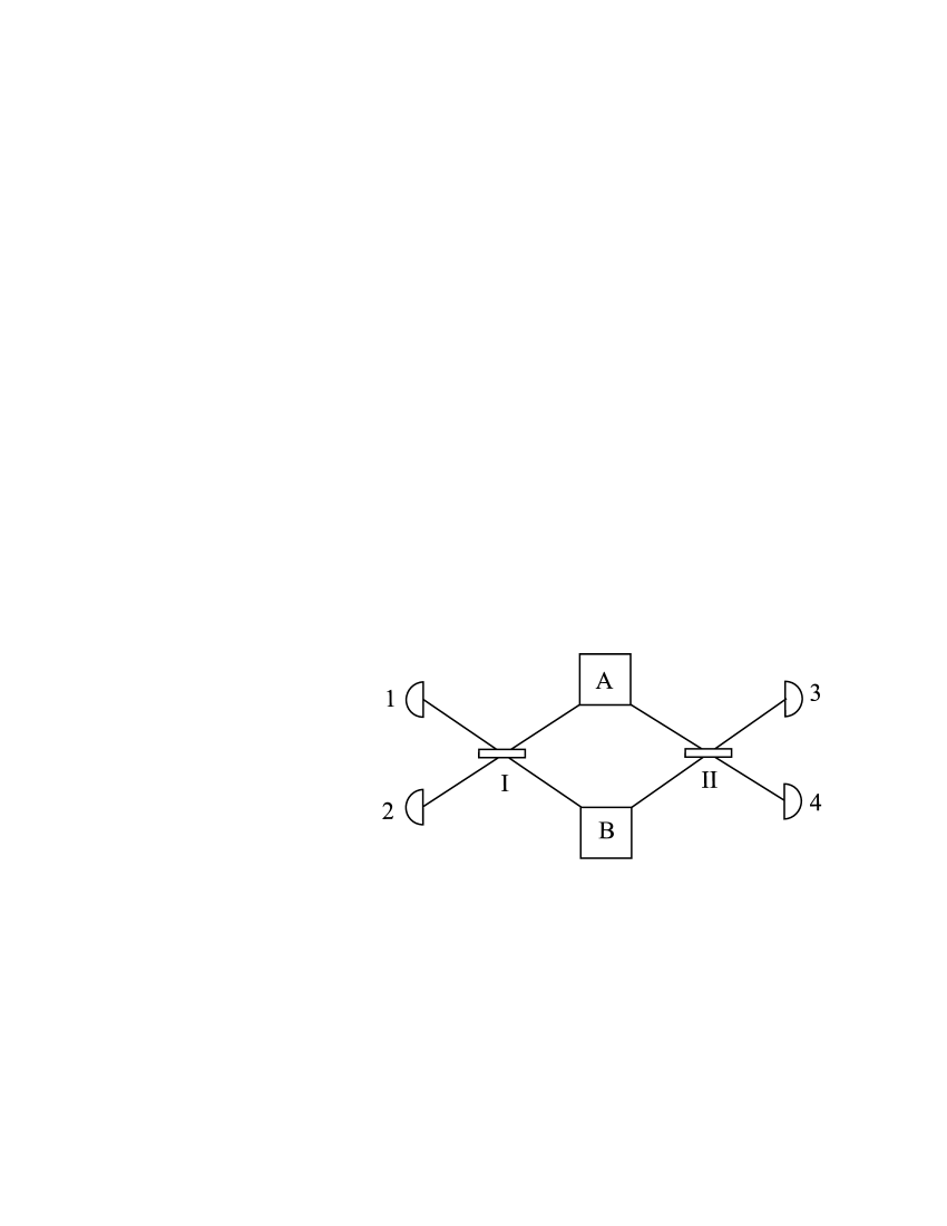
FIG. 1.: Sketch of setup with two decaying modes, where each mode emits particles into the input port of two different beam splitters.

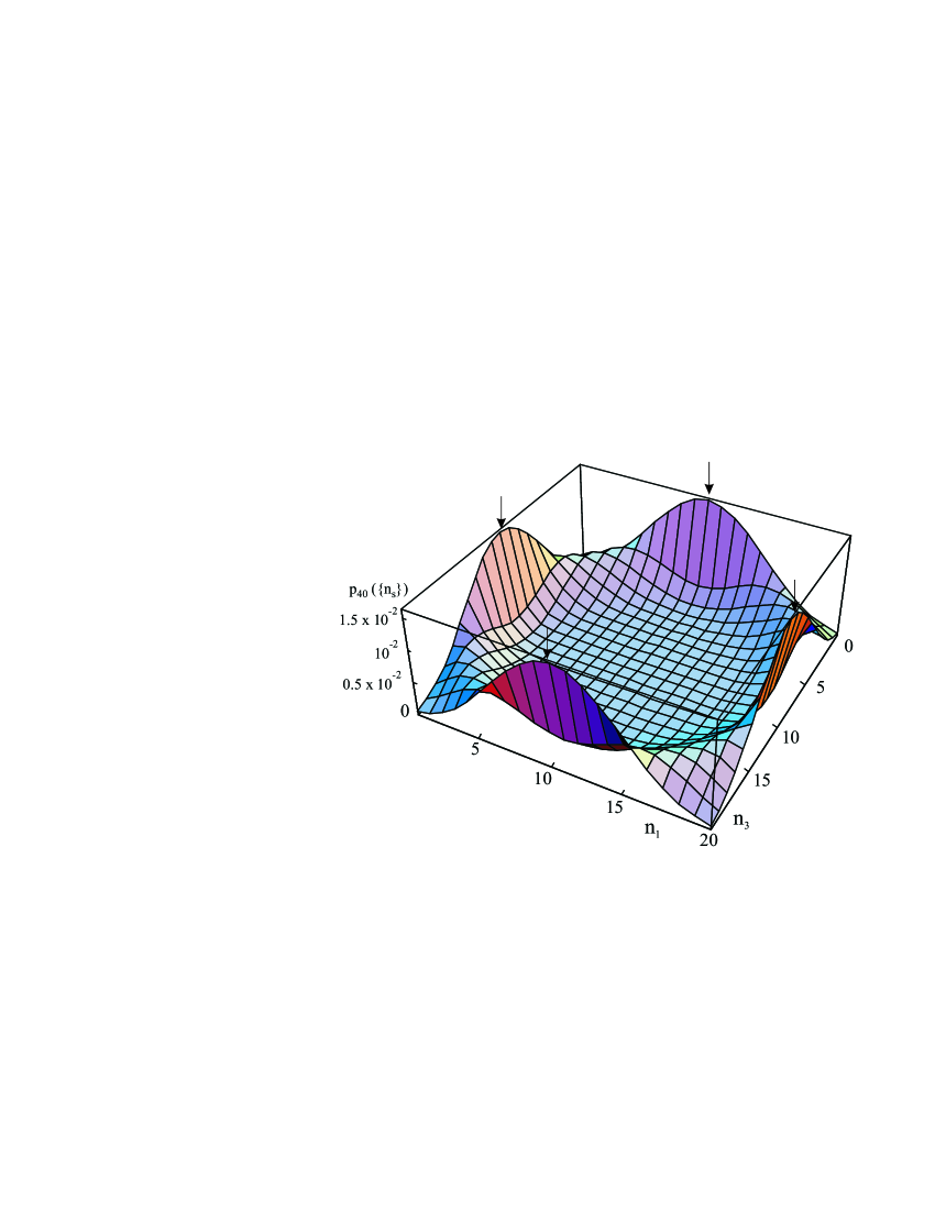
FIG. 2.: The probability distribution $p_{L}(\{n_{s}\})$ versus $n_{1}$ and $n_{3}$ for equal number of detections through both beam splitters. Here $L=40$ and $\xi=\pi/2$. The most probable histories are marked.

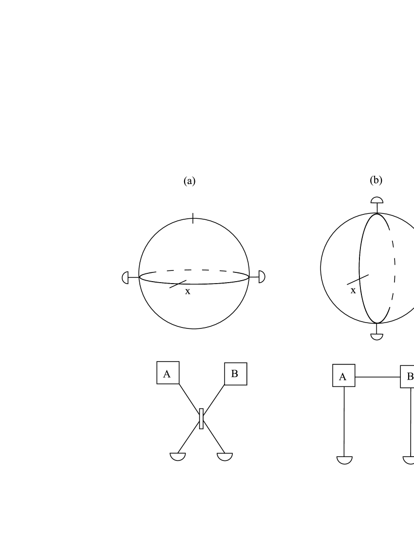
FIG. 3.: (a) emitted particles are detected directly, without the use of beam splitters; (b) emitted particles re detected through a beam splitter. For each case, the position of the detectors on the Bloch sphere, and the distribution of the state before detection are also shown.

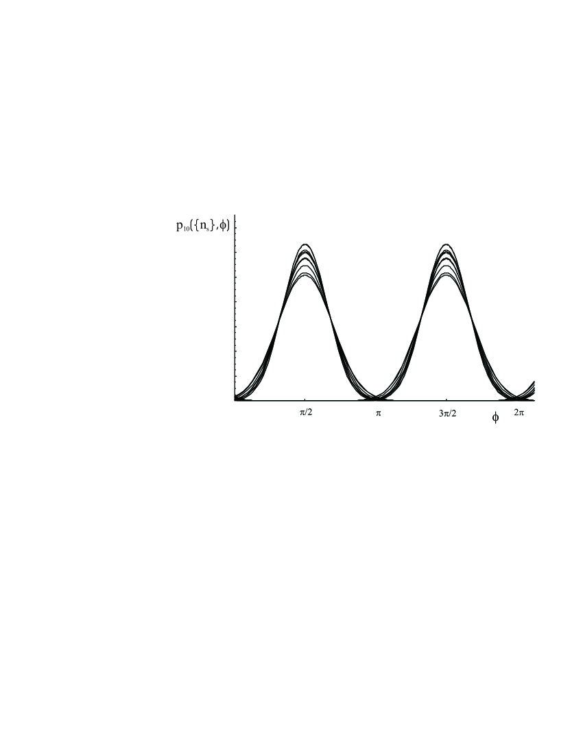
FIG. 4.: Relative phase distributions for two coupled modes after $L=10$ detections. Each curve of the ten curves corresponds to a different realization of the randomly selected detection times.

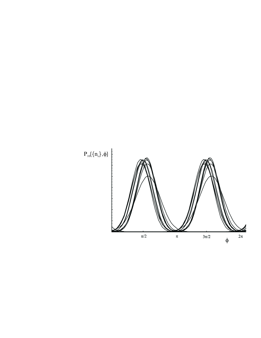
FIG. 5.: Same as fig. 4, now for two coupled modes at different energy. Coupling strength and energy splitting specified by $\varepsilon/\delta=1/4$.

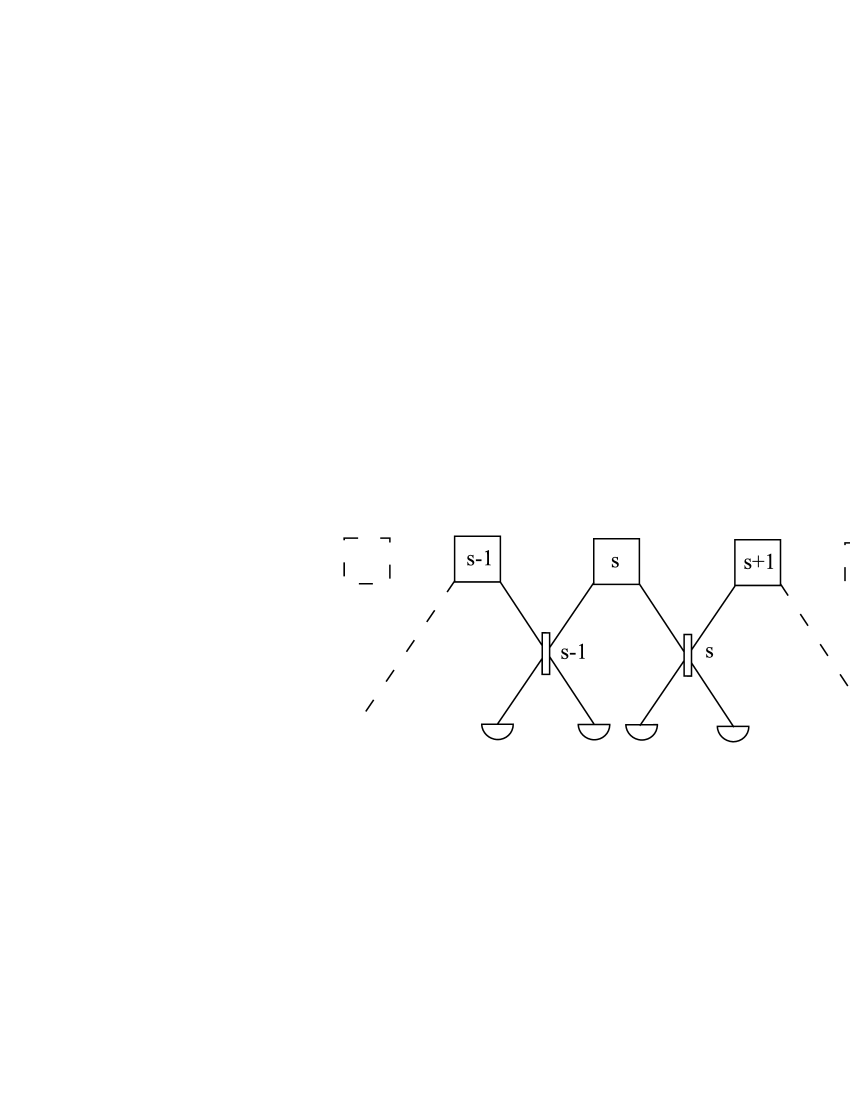
FIG. 6.: Sketch of setup with a linear chain of modes

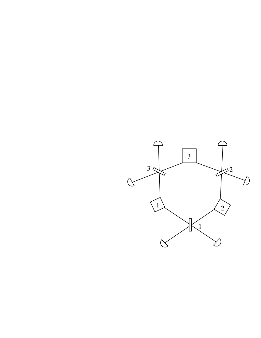
FIG. 7.: Sketch of setup with 3 modes arranged on circular chain.

- [1] J. Javanainen and S. M. Yoo, Phys. Rev. Lett. 76, 161 (1996).
- [2] M. R. Andrews, C. G. Townsend, H.-J. Miesner, D. S. Durfee, D. M. Kurn and W. Ketterle, Science 275, 637 (1997).
- [3] D. S. Hall, M. R. Matthews, C. E. Wieman and E. A. Cornell, Phys. Rev. Lett. 81, 1543 (1998).
- [4] J. I. Cirac, C. W. Gardiner, M. Naraschewski and P. Zoller, Phys. Rev. A 54, 3714 (1996).
- [5] J. Ruostekoski and D.F. Walls, Phys. Rev. A 58, 50 (1998).
- [6] J.A. Dunningham, S. Bose, L. Henderson, V. Vedral and K. Burnett, Phys. Rev A 65, 064302 (2002).
- [7] A.P. Hines, R.H. McKenzie and G.J. Milburn, Phys. Rev. A 67, 013609 (2003).
- [8] E.L. Bolda, S.M. Tan and D.F. Walls, Phys. Rev. Lett. 79, 4719 (1997).
- [9] Y. Castin and J. Dalibard, Phys. Rev. A 55, 4330 (1997).
- [10] G. Nienhuis, J. Phys. A 34, 7867 (2001).
- [11] A. J. Leggett and F. Sols, Found. Phys. 21, (1991) 353.
- [12] J. A. Dunningham and K Burnett, J. Phys. B: At. Mol. Opt. Phys. 33, 3807 (2000).
- [13] F. T. Arecchi, E. Courtens, R. Gilmore and H. Thomas, Phys. Rev. A 6, 2211 (1972).
- [14] C. W. Gardiner, Quantum Noise (Springer, Berlin, 1991).
- [15] L. Mandel and E. Wolf, Optical Coherence and Quantum Optics (Cambridge University Press, Cambridge, 1995).
- [16] N. Tsukada, Phys. Rev. A 65, 063608 (2002).