Quantum Heat Engines, the Second Law and Maxwell’s Daemon

Abstract

We introduce a class of quantum heat engines which consists of two-energy-eigenstate systems, the simplest of quantum mechanical systems, undergoing quantum adiabatic processes and energy exchanges with heat baths, respectively, at different stages of a cycle. Armed with this class of heat engines and some interpretation of heat transferred and work performed at the quantum level, we are able to clarify some important aspects of the second law of thermodynamics. In particular, it is not sufficient to have the heat source hotter than the sink, but there must be a minimum temperature difference between the hotter source and the cooler sink before any work can be extracted through the engines. The size of this minimum temperature difference is dictated by that of the energy gaps of the quantum engines involved. Our new quantum heat engines also offer a practical way, as an alternative to Szilard’s engine, to physically realise Maxwell’s daemon. Inspired and motivated by the Rabi oscillations, we further introduce some modifications to the quantum heat engines with single-mode cavities in order to, while respecting the second law, extract more work from the heat baths than is otherwise possible in thermal equilibria. Some of the results above are also generalisable to quantum heat engines of an infinite number of energy levels including 1-D simple harmonic oscillators and 1-D infinite square wells.

I Introduction

The second law has started out as a “no-go” statement against a certain class of perpetual machines but is now a pillar of modern physics, supported by experimental evidence without exception so far. While the first law of thermodynamics is a statement of quantity about energy conservation, the second law is a statement of quality about what kinds of energy transformations are and are not allowed. T,here are several classical statements of the second law Zemansky (1968); Callen (1960):

• Kelvin-Planck: No process is possible whose sole result is the absorption of heat from a reservoir and the conversion of this heat into work.

• Clausius: No process is possible whose sole result is the transfer of heat from a cooler to a hotter body.

• Entropy Maximum Postulate: The entropy of a closed system never decreases in any process.

The first two statements above can be shown to be equivalent by the introduction of intermediate heat engines. And the last postulate requires the introduction of entropy which is a function of extensive parameters of a composite system, defined for all equilibrium states and having certain properties.

Entropy of a composite system in a macro-state can be linked, in statistical physics, to the statistics of the many micro-states that correspond to the same macro-state. In order to satisfy the statistical nature of entropy and to derive the principle of increasing entropy, several fundamental assumptions are required Planck (1998):

• The composite system has a large number of components (atoms, molecules, etc.).

• These components can be divided into a small number of classes of indistinguishable components. (In fact, were every molecule of a gas assumed to be different from each other then statistical physics would become fairly simple but useless as it would not be able to account for the non-decreasing flow of entropy.)

• Boltzmann’s fundamental hypothesis Pauli (2000): all micro-states are equally probable. This is termed as elementary disorder by Planck and has been generalised to the quantum domain as the hypotheses of equal a priori probabilities and random a priori phases for the quantum states of a system Tolman (1979). All of these can be subsumed by the (somewhat stronger) ergodic hypothesis Pauli (2000) which postulates that the dynamical time average is equal to the ensemble average (of appropriate ensembles), except for a number of exceptional initial conditions of relatively vanishing importance.

No matter how reasonable the last assumption may be, it should be pointed out that those hypotheses are not a part of but are extra to the first principles of quantum mechanics.

The second law was indeed the motivation and the philosophical reason for Max Planck to introduce the concept of energy quanta in his solution for the puzzle of black-body radiation Planck (1998). His line of reasoning can be rephrased as follows: the second law is about irreversibility in nature; irreversibility does nothing but defines a preference of the more probable over the less probable; and the probability assignment for physical states (in order to have the more and the less probables) requires those states to belong to a distinguishable variety of possibilities. This led Planck to the conclusion that the atomic hypothesis must be necessary. And the rest was history; the concept of quanta was then born as the states of discrete homogeneous elements. In that context, the study of heat engines in the quantum domain in relation to the second law is a contribution to a completion of the circle that was started at the beginning of the last century.

Present technology now allows for the probing and/or realisation of quantum mechanical systems of mesoscopic and even macroscopic sizes (like those of superconductors, Bose-Einstein condensates, etc.) which can also be restricted to a relatively small number of energy states. It is thus important to study these quantum systems directly in relation to the second law. Our study, started with Kieu (2004) and further expanded in this paper, is part of a growing body of investigations into quantum heat engines Zurek (2003); Geva and Kosloff (1992); Feldmann et al. (1996); Feldmann and Kosloff (2000); Bender et al. (2000); Opatrny and Scully (2002); Scully et al. (2003); Arnaud et al. (2003); Maruyama et al. (2005); Quan et al. (2005). Explicitly, the only principles we will need are those of the Schrödinger equation, the Born probability interpretation of the wavefunctions and the von Neumann measurement postulate von Neumann (1955). In particular, we will not exclude, but will make full use of, any exceptional initial conditions, as long as they are realisable physically. However, without a better understanding of the emergence of classicality from quantum mechanics, we will also have to assume the thermal equilibrium Gibbs distributions for the heat baths that are coupled to the quantum systems. This assumption is related to the fundamental assumptions mentioned above and is extra to those of quantum mechanics. Even though we do not impose this extra assumption on the quantum mechanical systems, the steady-state distributions for the systems will eventually reach the Gibbs distributions in time because of the coupling with the heat baths, see eq. (14) below.

In order to introduce a class of heat engines operating entirely in the framework of quantum mechanics, we will need a quantum interpretation of the transfer of heat and performance of work in the next Section. This interpretation is also necessary for a review of the second law and for a possible realisation, as an alternative to Szilard’s engine, of Maxwell’s daemon in Sections III and IV. The quantum heat engines are then considered next both in thermal equilibrium and also in thermal non-steady states, in Sections V and VI. We find from these quantum considerations that even though the second law is not violated in a broad sense, it needs some refinements and clarifications. We also demonstrate that more work can be extracted by the engines in non-steady states than otherwise is possible in thermal equilibrium, Section VII. Section VIII provides an explicit numerical illustration of such capability. We then discuss Maxwell’s daemon further in Section IX as the reason behind any violation of the second law were we ever able to control the quantum phases of the heat baths. Sections X and XI contain some generalised results for quantum heat engines with simple harmonic oscillators and infinite square wells, respectively, all in one dimension. Finally, we end the paper with some concluding remarks in the final Section XII.

II Quantum identifications of heat exchanged and work performed

The expectation value of the measured energy of a quantum system with discrete energy levels is

$$U=\langle E\,\rangle = \sum_{i}p_{i}\,E_{i},$$ (1)

in which $E_{i}$ are the energy levels and $p_{i}$ are the corresponding occupation probabilities. Infinitesimally,

$$dU = \sum_{i}\{E_{i}\,dp_{i}+p_{i}\,dE_{i}\},$$ (2)

from which we make the following identifications for infinitesimal heat transferred ${\mathchar 22\relax\mkern-11.0mud}Q$ and work done ${\mathchar 22\relax\mkern-11.0mud}W$

$${\mathchar 22\relax\mkern-11.0mud}Q := \sum_{i}E_{i}\,dp_{i},$$

$${\mathchar 22\relax\mkern-11.0mud}W := \sum_{i}p_{i}\,dE_{i}.$$ (3)

Mathematically speaking, these are not total differentials but are path dependent. These expressions interpret heat transferred to or from a quantum system as the change in the occupation probabilities but not in the change of the energy eigenvalues themselves; and work done on or by a quantum system as a redistribution of the energy eigenvalues but not of the occupation probabilities of each energy level. Together with these identifications, equation (2) can be seen as just an expression of the first law of thermodynamics, $dU={\mathchar 22\relax\mkern-11.0mud}Q+{\mathchar 22\relax\mkern-11.0mud}W$.

The above link between the infinitesimal heat transferred to the infinitesimal change of occupation probabilities is in accord with, or at least is not in contradiction to, the thermodynamic link between heat and entropy, ${\mathchar 22\relax\mkern-11.0mud}Q=T\,dS$, in combination with the statistical physical link between entropy and probabilities, $S=-k\sum_{i}p_{i}\,\ln p_{i}$. On the other hand, expression (3) linking work performed to the change in energy levels agrees with the fact that work done on or by a system can only be performed through a change in the generalised coordinates of the system, which in turn gives rise to a change in the distribution of the energy levels Schrödinger (1989).

III A class of quantum heat engines

The quantum heat engines considered herein are just two-energy-level quantum systems, the simplest of quantum mechanical systems, operated in a cyclic fashion described below. (They are the quantum analogue of the classical Otto engines and are readily extendable to systems of many discrete energy levels.) They could perhaps be realised with coherent macroscopic quantum systems like, for instance, a Bose-Einstein condensate confined to the bottom two energy levels of a trapping potential. The exact cyclicity will be enforced to ensure that upon completing each cycle all the output products of the engines are clearly displayed without any hidden effect.

A cycle of the quantum heat engine consists of four stages:

• Stage 1: The system has some probability to be in the lower state prior to some kind of contact (whose nature will be discussed later on) with a heat bath at temperature $T_{1}$. After some time interval, there is a probability that the system receives some energy from the heat bath to jump up an energy gap of $\Delta_{1}$ to be in the upper state. According to the identification above, only heat is transferred in this stage to yield a change in the occupation probabilities, and no work done as there is no change in the values of the energy levels. This stage is depicted on the left hand side of Fig. 1.

• Stage 2: The system is then isolated from the heat bath and undergoes a quantum adiabatic expansion, whose nett result is to reduce the energy gap from $\Delta_{1}$ to a smaller value $\Delta_{2}$. In this stage, provided the expansion rate is sufficiently slow according to the quantum adiabatic theorem Messiah (1999), the occupation probabilities for the two states remain unchanged. The system may perform an amount of work. This is depicted as the upper branch of Fig. 1 running from left to right. Note that there is no change in probability so there is no heat transferred; that is, a quantum adiabatic process implies a thermodynamic adiabatic process (but not the other way around, in general).

• Stage 3: The system is next brought into some kind of contact with another heat bath at temperature $T_{2}$ for some time. There is a probability that it releases some energy to the bath to jump down the gap $\Delta_{2}$ to be in the lower state. This is depicted on the right hand side of Fig. 1. Some heat is thus transferred but no work is performed in this stage.

• Stage 4: The system is removed from the heat bath nd undergoes a quantum adiabatic contraction, whose nett result is to increase the energy gap from $\Delta_{2}$ back to the previously larger value $\Delta_{1}$. This is depicted as the lower branch of Fig. 1 running from right back to left. In this stage an amount of work is done on the system.

Ideal quantum adiabatic processes are employed here because they yield, on the one hand, the maximum amount of work performable by the systems in stage 2 (as the transition probabilities to the lower state in that stage can be made vanishingly small according to the quantum adiabatic theorem), but yield the minimum amount of work performable on the systems (by some external agents) in stage 4, on the other hand. In each cycle the amount of work done by the system is $(\Delta_{1}-\Delta_{2})$, which is also the nett amount of heat it absorbs. Note that we need not and have not assigned any temperature to the quantum system; all the temperatures are properties of the heat baths, which in turn are assumed to be in the Gibbs state.

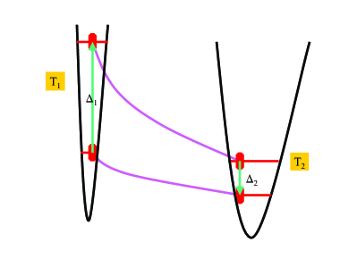
Figure 1: On the left hand side, a two-state quantum system in the lower state comes into contact with a heat bath at temperature $T_{1}$ for some time until it absorbs an amount of energy $\Delta_{1}$ to jump into the upper state. Next in the passage to the right hand side, the system undergoes a quantum adiabatic process, remaining in the upper state, and performs work on the relaxing potential wall. On the right hand side, the system comes into contact with another heat bath at temperature $T_{2}$ for some time until it releases an amount of energy $\Delta_{2}$ to jump back to the lower state. In the final passage to the left hand side to complete a cycle of the heat engine, the system undergoes another quantum adiabatic process in which it remains in the lower state and work is done on the system by the compressing potential wall.

However, in the operation above, the absorption and release of energy in stages 1 and 3 occur neither definitely nor deterministically. Quantum mechanics tells us that they can only happen probabilistically; and the probabilities that such transitions take place depend on the details of the interactions with and some intrinsic properties (namely, the temperatures) of the heat baths.

Let ${p}_{u}^{\,(1,2)}$ be the probabilities for the system to be in the upper level at the beginning of stages 2 and 4, respectively. The nett work done by our quantum heat engines in the two quantum adiabatic passages in stages 2 and 4 is

$$\Delta W = \left(\int_{\mbox{\small left $\to$ right}}+\int_{\mbox{\small right $\to$ left}}\right)\sum_{i}p_{i}\,dE_{i},$$ (4)

$$= \left({p}_{u}^{\,(1)}-{p}_{u}^{\,(2)}\right)\left(\Delta_{2}-\Delta_{1}\right).$$

We will make full use of this simple expression in the Sections below.

By the weak law of large numbers, probability reflects the relative occurrence frequency of an event in a large number of repetitions. In the case of thermal equilibrium with only one single heat bath ($T_{1}=T_{2}$), even with a small probability $\tilde{p}_{u}^{\,(1)}(1-\tilde{p}_{u}^{\,(2)})$ the system could be in the upper level in stage 2 and in the lower level in stage 4, where $\tilde{p}$ is the thermal equilibrium probabilities in (5) below. The probability, however, diminishes exponentially for $n_{c}$ consecutive cycles, $(\tilde{p}_{u}^{\,(1)}(1-\tilde{p}_{u}^{\,(2)}))^{n_{c}}$, in all of which the system would perform nett work on the environment. As a result, there are certain cycles whose sole result is the absorption of heat from a reservoir and the conversion of this heat into work, of the amount $(\Delta_{1}-\Delta_{2})$!

This amounts to a violation of the Kelvin-Planck statement of the second law due to the explicit probabilistic nature of quantum mechanical processes. This violation of classical statements for the second law, however, occurs only randomly, with some vanishingly small probability in the longer term, and thus is not controllable – neither harnessible nor exploitable.

This may seem non-surprising given the statistical nature of the second law, but it is somewhat different from the usual scenario of violation of the second law by statistical fluctuations in the bulk. One example of this latter scenario is the instantaneous concentration of all the gas molecules in a big room into one of its corners. Mathematically, this configuration is permissible due to the existence of the Poincaré cycles in mechanics, but statistical physics effectively rules this out (gives it a vanishing probability) by invoking extra assumptions and hypotheses as mentioned in Section I. The scenario with our quantum heat engines is different in that it only involves a single (macro) quantum system with physically realisable quantum mechanical probabilities, and without any extra hypothesis. The subtle difference between the two cases is in the time average for a single system, on the one hand, and the bulk average for systems having many subcomponents, on the other.

IV A realisation of Maxwell’s Daemon

However, there exists a sure way to always extract work, to the amount of $(\Delta_{1}-\Delta_{2})$, in each completable “cycle” described in Section III. In order to eliminate the probabilistic uncertainty in the thermalising contacts with heat baths,

• we prepare the system to be in the lower state prior to stage 1;

• we perform an energy measurement after stage 1 and then only let the engine continue to stage 2 subject to the condition that the measurement result confirms that the system is in the upper state; if this is not the case, we go back to the last step above;

• we next perform another measurement after stage 3 and then only let the engine continue to stage 4 subject to the condition that the measurement result confirms that the system is in the lower state; if this is not the case, we go back to the last step above.

All the steps above is to ensure ${p}_{u}^{\,(1)}=1$ and ${p}_{u}^{\,(2)}=0$, irrespective of the heat bath temperatures, and thus to be always able to derive maximum work according to (4). That is, all this can be carried out even for the case $T_{1}\leq T_{2}$ to always extract, in a controllable manner, some work which would have been otherwise prohibited by the second law.

This apparent violation of the second law is analogous to that of Szilard’s one-atom engine and is nothing but the result of an act of Maxwell’s daemon Leff and Rex (1990). Indeed, the condition of strict cyclicity of each engine’s cycle is broken here. After each cycle the measurement apparatus, being a Maxwell’s daemon, has already registered the conditioning results which are needed to determine the next steps of the engine’s operation. In this way, there are extra effects and changes to the register/memory of the apparatus, even if we assume that the quantum measurement steps themselves cost no energy and leave no nett effect anywhere else. To remove these remnants in order to restore the strict cyclicity, we would need to bring the register back to its initial condition by erasing any information obtained in each of the cycles, either by resetting its bits or by thermalising the register with some heat bath. Either way, extra effects are inevitable, namely an amount of heat of at least $kT\ln 2$ will be released per bit erased. This is the Landauer principle which saves the second law. More extensive discussions and debates on these issues can be found in the literature Leff and Rex (1990), and in particular in the quantum version of Szilard’s engine by Zurek Zurek (2003). Lloyd in Lloyd (1997) has analysed carefully and in detailed the Landauer principle behind the working of Maxwell’s daemon entirely in the framework of quantum mechanics. Maxwell’s daemon has also been discussed Nielsen et al. (1998) in the context of quantum error correction in quantum computation.

Our quantum heat engines could thus provide, in a different way to Szilard’s engine, a feasible and quantum mechanical way to realise Maxwell’s daemon.

V Thermal steady states

We have pointed out in Section  III that there are random instances where our quantum heat engines can extract heat from a single heat bath and totally turn that into work or, equivalently, can transfer heat from a cold to a hot source (and may also do some work at the same time). Nonetheless, on the average, there is no violation of the second law.

If the system is allowed to thermalise with the heat baths in stages 1 and 3, the thermal equilibrium probabilities for the two energy levels only depend on the relevant temperatures and the energy gaps, but not on the initial states when the system is brought into contact with the heat bath, see (14) below. More explicitly, the probability $\tilde{p}_{u}^{\,(1)}$ to have the system in the upper state at the end of stage 1 after being thermalised with the heat bath at temperature $T_{1}$, and $\tilde{p}_{u}^{\,(2)}$ at the end of stage 3 after being thermalised with the heat bath at temperature $T_{2}$, respectively, are

$$\tilde{p}_{u}^{\,(i)} = 1/\left(1+\exp\{{\Delta_{i}}/{kT_{i}}\}\right),\mbox{ for }i=1,2.$$ (5)

These probabilities are definitely non-zero and bounded by $0.5$. From which, the work derived from (4) is

$$\Delta W_{\rm th} = \left(\tilde{p}_{u}^{\,(1)}-\tilde{p}_{u}^{\,(2)}\right)\left(\Delta_{2}-\Delta_{1}\right).$$ (6)

This is negative (that is, work has been performed by our engines), given that $\Delta_{1}>\Delta_{2}$, if and only if, as can be seen from (5),

$${T_{1}} > T_{2}\left(\frac{\Delta_{1}}{\Delta_{2}}\right),$$ (7)

which is to be compared with the necessary condition of the classical statement of the second law that $T_{1}$ is simply greater than $T_{2}$.

One might think that the last result is just another equivalent restatement of the second law by arguing that the entropy decreased in the heat bath in stage 1 must be, according to the usual statement of the second law, less than the entropy increased in the other heat bath in stage 3,

$$\frac{\Delta Q_{2}}{T_{2}} > \frac{\Delta Q_{1}}{T_{1}}\,,$$ (8)

and by assuming that $\Delta Q_{i}=\Delta_{i}$, for both $i$, upon which (7) would have immediately followed. However, this assumption is not justifiable because the heat $\Delta Q_{1}$ released by the hot heat bath, on the average, cannot be the same as the energy gap $\Delta_{1}$ of the system at that point; and likewise for the heat absorbed by the colder reservoir. These heat amounts must be, on the average, less than the corresponding energy gaps because the heat absorbed/released by the quantum system must be moderated by the change in occupation probabilities (see (3)), but such a change in the occupation probability for a specific level is always less than one. In other words, the energy gaps $\Delta_{i}$’s are the maximum energy transfers possible in any exchange but the probability distributions in thermal equilibrium will not allow those maximum values to be reached. However, the result (7) is consistent with the second law (8) in the sense that it can be derived from (8) if $\Delta Q_{i}$ is proportional to $\Delta_{i}$ and if the proportionality constants (which are less than one) are the same for both $i=1,\,2$. But such a proportionality is extra ingredient to the second law (8), and is a consequence of the same cause that also leads to (7). Consequently, our derived result (7) is a refinement of the classical statement of the second law, and not simply a restatement in another equivalent form.

The expressions (4) and (7) not only confirm the broad validity of the second law but also refine the law further in specifying how much $T_{1}$ needs to be larger than $T_{2}$ before some work can be extracted. In other words, work cannot be extracted, on the average, even when $T_{1}$ is greater than $T_{2}$ but less than $T_{2}(\Delta_{1}/\Delta_{2})$, in contradistinction to the classical requirement that $T_{1}$ only needs to be larger than $T_{2}$. The refinement factor $(\Delta_{1}/\Delta_{2})$ is necessarily greater than unity (by the requirement of energy conservation) and is dictated by the quantum structure of the heat engines. This result may be extended to multi-level quantum heat engines with appropriate energy gaps, provided the quantum energy levels involved are discrete. (See Quan et al. (2005), however.) We show in Section X the equivalent condition, ${T_{1}}>T_{2}\left({\omega_{1}}/{\omega_{2}}\right)$, for quantum simple harmonic oscillators–where $\omega_{1}$ and $\omega_{2}$ are, respectively, the frequencies of the oscillators in the equivalence of stages 1 and 3 above (with $\omega_{1}>\omega_{2}$).

The efficiency of the two-state engines is found to be

$$\eta_{q} = \frac{\Delta W_{\rm th}}{Q_{\rm in}}=\left(1-\frac{\Delta_{2}}{\Delta_{1}}\right),$$ (9)

which is independent of temperatures and is the maximum available within the law of quantum mechanics. (A similar expression, but through a specific context, was also obtained in Scovil and Schulz-DuBois (1959).) This expression also serves as the upper bound, with appropriate $\Delta_{1}$ and $\Delta_{2}$, of the efficiency of any quantum heat engine because the work performed by our heat engines through their quantum adiabatic processes is the maximum that can be extracted.

The efficiency is, as a consequence of (7), less than that of the classical Carnot engines, $\eta_{C}$,

$$\eta_{q}<1-T_{2}/T_{1}\equiv\eta_{C}.$$ (10)

This is in agreement with a general fact established by Lloyd Lloyd (1997) that quantum efficiency must be reduced as more information is obtained about the system either by measurement or decoherence. Lloyd argues that when the system is in a fully measured or decohered state (that is, when the density matrix is already diagonal with respect to a measured or preferred basis) then no further information can be introduced, whence the Carnot efficiency might thus be achieved.

However, the limiting Carnot efficiency may also be approached in the quantum mechanical framework through the limit of an infinite number of quantum adiabatic processes Geva and Kosloff (1992); Bender et al. (2000); Arnaud et al. (2003). We illustrate this fact for our quantum heat engines in Fig. 2. A similar discussion can also be found with the heat engines of Arnaud et al. (2003).

Fig. 2 depicts the inverses of (5),

$$\Delta = kT\ln\left(\frac{1}{\tilde{p}}-1\right),$$ (11)

with the labels $T_{1}$ and $T_{2}$ correspond to the two temperatures. The rectangle $ABCD$ represents a particular operation of our quantum heat engines between two heat baths $T_{1}$ and $T_{2}$ – with stage 2 represented by the segment $AB$ (which is adiabatic with no change in the probability); stage 3 by $BC$ (no work done with constant energy gap); stage 4 by $CD$; and stage 1 by $DA$, completing an engine cycle. The area of $ABCD$, by virture of (4), represents the work derivable from this operation, which is less than the area bounded by the two vertical lines $AB$ and $CD$ and the two curves, which in turn is the work derivable from a corresponding Carnot engine also operated between the two temperatures.

Now, we modify our heat engines to have $AB$ as the adiabatic expansion, $BC$ the heat exchange, $CE$ the adiabatic compression, $EF$ the heat exchange, and so on. When the division becomes finer and finer with more and more steps, the area of the (red) zigzag polygon will approach, from the inside, that of the irregular shape bounded by the outermost two vertical lines and two horizontal curves. This is the limit when our modified quantum heat engine can have both the same work output per cycle and the same efficiency as those of a corresponding Carnot engine.

We think that this approach will have some interesting consequences in the context of quantum information and hope to be able to present further analysis on this limiting scenario elsewhere.

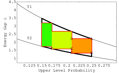
Figure 2: Even though the quantum efficiency is always bounded by the Carnot efficiency, a quantum heat engine with asymptotically infinite number of quantum adiabatic steps can have both its efficiency and work output per cycle approaching those of the latter. This can be seen when the area of the (red) zigzag polygon approaches, from the inside, that of the irregular shape bounded by the two outermost vertical lines and the curves labeled $T_{1}$ and $T_{2}$. See text for further explanation.

VI Transition to thermal steady states

Given that the efficiency is bounded by that of Carnot engines, which is another manifestation of the second law, can we derive more work (with a larger heat input so that the efficiency bound is maintained) than that obtainable from the thermal steady states? In the transient states approaching the thermal equilibria in stages 1 and 3 of a quantum heat engines’ cycle, the density matrix elements with the upper eigenstate $|u\rangle$ and lower $|l\rangle$ satisfy the following equations Scully and Zubairy (1997), for $i=1,2$,

$$\partial_{t}\rho_{uu}^{\,(i)} = -(\bar{n}_{i}+1)\Gamma\rho_{uu}^{\,(i)}+\bar{n}_{i}\Gamma\rho_{ll}^{\,(i)},$$

$$\partial_{t}\rho_{ll}^{\,(i)} = -\bar{n}_{i}\Gamma\rho_{ll}^{\,(i)}+(\bar{n}_{i}+1)\Gamma\rho_{uu}^{\,(i)},$$ (12)

$$\partial_{t}\rho_{ul}^{\,(i)} = \partial_{t}\left(\rho_{lu}^{\,(i)}\right)^{*}=-\left(\bar{n}_{i}+\frac{1}{2}\right)\Gamma\rho_{ul}^{\,(i)},$$

under the Markovian assumption and the rotating-wave approximation and in which the heat bath is treated as a collection of infinite number of simple harmonic oscillators. In the above, $\Gamma$ is the decay rate and we have assumed that the thermal average boson number in the heat bath having frequency $\nu=\Delta_{i}/h$ is

$$\bar{n}_{i} = \frac{1}{e^{\frac{\Delta_{i}}{kT_{i}}}-1}\,.$$ (13)

The solution for the differential equations above with the heat bath at $T_{i}$ is

$$\rho_{uu}^{\,(i)}(t) = e^{-(2\bar{n}_{i}+1)\Gamma t}\left(\rho_{uu}^{\,(i)}(0)-\tilde{p}_{u}^{\,(i)}\right)+\tilde{p}_{u}^{\,(i)}.$$ (14)

Let the system stay in contact with the heat bath at temperature $T_{1}$ in stage 1 for a time $\tau_{1}$ (without achieving thermalisation); and for a time $\tau_{2}$ at $T_{2}$ in stage 2. The cyclicity of the quantum heat engines requires that

$$\rho_{uu}^{\,(1)}(0) = \rho_{uu}^{\,(2)}(\tau_{2}),$$

$$\rho_{uu}^{\,(2)}(0) = \rho_{uu}^{\,(1)}(\tau_{1}).$$ (15)

This requirement together with that of $\tilde{p}_{u}^{\,(1)}>\tilde{p}_{u}^{\,(2)}$ imply, from (14),

$$0< \rho_{uu}^{\,(1)}(\tau_{1})-\rho_{uu}^{\,(2)}(\tau_{2}) <\tilde{p}_{u}^{\,(1)}-\tilde{p}_{u}^{\,(2)},$$ (16)

for finite $\tau_{1}$ and $\tau_{2}$. Subsequently, the work, $\left|\Delta W_{\rm tr}\right|$, that can be derived from transient states at finite $\tau_{1}$ and $\tau_{2}$ is always less than that from thermal equilibrium, $\left|\Delta W_{\rm th}\right|$,

$$\left|\Delta W_{\rm tr}\right| = \left(\rho_{uu}^{\,(1)}(\tau_{1})-\rho_{uu}^{\,(2)}(\tau_{2})\right)\left(\Delta_{1}-\Delta_{2}\right),$$

$$< \left(\tilde{p}_{u}^{\,(1)}-\tilde{p}_{u}^{\,(2)}\right)\left(\Delta_{1}-\Delta_{2}\right),$$

$$< \left|\Delta W_{\rm th}\right|.$$

We suspect that, as long as the assumption of Gibbs distributions is made for the heat baths, a non-Markovian treatment or dropping the rotating wave approximation would not change this last result. Nonetheless, we present in the next Section a modification of the quantum heat engines which can better the work derivation than that which is maximally available from thermal equilibrium.

VII Maximising the work extraction

Inspired and motivated by the Rabi flopping for two-level systems, see Scully and Zubairy (1997), for example, we present in this Section a modification of the engines such that more work than usual can be derived from thermal heat sources (as contrast to a single-Fock-state field that drives the Rabi flopping), but at the same time more heat input would be needed in such a way that the Carnot efficiency is still a valid upper bound. That is, no violation of second law is claimed here despite of the enhanced work output.

A scenario for maximizing the work output from our quantum heat engines is as follows. Firstly, the system is prepared to be in the lower state and then subject to a radiation field in a Fock state which has exactly $n_{1}$ quanta with a frequency in resonance with the energy gap $\Delta_{1}$. After some fixed time $\tau_{1}$, depending on the system-field coupling strength and on the number $n_{1}$, Rabi oscillations driven by the radiation field will bring the system to the upper energy state with certainty. At this point the system can be removed from the field to perform some work in an adiabatic process which reduces the energy gap to $\Delta_{2}$. Then it is next subject to another field of Fock state $|n_{2}\rangle$ which has a frequency in resonance with the new gap $\Delta_{2}$. After some time $\tau_{2}$ the system will be in the lower state with certainty; upon which it can be decoupled for an adiabatic compression to complete a cycle of the operation.

In effect, the steps above will remove the probability difference factor in (4), ensuring that a nett work of $(\Delta_{1}-\Delta_{2})$ is derived in each cycle. The key point here, however, is that a Fock-state field is not a thermal field, and extra work or extra information would be required to maintain the Fock state such that the nett book keeping (when full cyclicity is strictly enforced) will show that we cannot ultimately violate the second law.

Let us exploit this Rabi mechanism and see how it will behave in a thermal field.

A cycle of the modified quantum heat engine is depicted in Fig. 3.

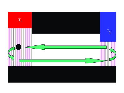
Figure 3: A single-mode cavity is in thermal equilibrium with a bath of black-body radiation at temperature $T_{1}$. A two-state quantum system spends some time in the cavity whose mode matches the energy gap $\Delta_{1}$ between its two states. After some prescribed time, it leaves the cavity and performs work in an quantum adiabatic process. It then enters another single-mode cavity which is in thermal equilibrium with another bath of black-body radiation at temperature $T_{2}$ and whose mode matches the new energy gap $\Delta_{2}$. After a carefully controlled time, it leaves the cavity and moves quantum adiabatically back to the first cavity, having work done on it to have the energy gap increases back to $\Delta_{1}$. With precise control of the time duration spent in each cavity, the system can extract more work in a cycle than it can if it is otherwise let to thermally equilibrate with the two heat baths in turn.

It also consists of four stages, of which stage 2 and stage 4 remain the same as described in Section III, whereas stages 1 and 3 are replaced respectively by:

• Stage 1’: The system has a probability $p_{u}^{\,(1)}(0)$ to be in its upper state. It is entered to a single-mode cavity which is tuned to match the energy gap $\Delta_{1}$ of the system and which is in thermal equilibrium with a heat bath at temperature $T_{1}$. The average occupation of the only mode survived in the cavity has thus a (Bose-Einstein) thermal distribution $\bar{n}_{1}$ given by expression (13). After some carefully controlled time interval $\tau_{1}$, the system is removed from the cavity to enter stage 2. The probability to find the system in it upper state is now $p_{u}^{\,(1)}(\tau_{1})$. Note that, as discussed previously, only heat could be transferred in this stage to yield a change in the occupation probabilities, and no work done as there is no change in the values of the energy levels. This stage is depicted on the left hand side of Fig. 3.

• Stage 3’: The system has a probability $p_{u}^{\,(2)}(0)$ to be in its upper state. It is entered into another single-mode cavity which is in thermal equilibrium with another heat bath at temperature $T_{2}$ and which is tuned to match the new energy gap $\Delta_{2}$ of the system. The average occupation of the only mode survived in the cavity has thus a (Bose-Einstein) thermal distribution $\bar{n}_{2}$ given by expression (13). After some carefully controlled time interval $\tau_{2}$, the system is removed from the cavity to enter stage 4. The probability to find the system in it upper state is now $p_{u}^{\,(2)}(\tau_{2})$. This is depicted on the right hand side of Fig. 3. Some heat is thus transferred but no work is performed in this stage.

With the quantum adiabatic processes in stage 2 and stage 4, the cyclicity of the heat engines demands that

$$p_{u}^{\,(1)}(0) = p_{u}^{\,(2)}(\tau_{2}),$$

$$p_{u}^{\,(2)}(0) = p_{u}^{\,(1)}(\tau_{1}).$$ (18)

On the other hand, the exit probability can be obtained as, with $i=1,2$,

$$p_{u}^{\,(i)}(t) = \left(\mbox{initial probability in }|u_{i}\rangle\right)\times\left(\mbox{transition probability from }|u_{i}\rangle\mbox{ to }|u_{i}\rangle\mbox{ in }t\right)+$$ (19)

$$\left(\mbox{initial probability in }|l_{i}\rangle\right)\times\left(\mbox{transition probability from }|l_{i}\rangle\mbox{ to }|u_{i}\rangle\mbox{ in }t\right),$$

$$= p_{u}^{\,(i)}(0)|\langle u_{i}|\psi_{u}^{\,(i)}(t)\rangle|^{2}+\left(1-p_{u}^{\,(i)}(0)\right)|\langle u_{i}|\psi_{l}^{\,(i)}(t)\rangle|^{2}.$$

$|\psi_{u(l)}^{\,(i)}(t)\rangle$ is the state which starts out in the upper (lower) state – i.e., $|\psi_{u}^{\,(i)}(0)\rangle=|u_{i}\rangle$ and $|\psi_{l}^{\,(i)}(0)\rangle=|l_{i}\rangle$ in the cavity at temperature $T_{i}$.

With the thermal distribution (13) assumed for the heat baths in contact with the cavities, the probability to find exactly $n$ photons of frequency $\Delta_{i}/h$ in the cavity at temperature $T_{i}$ is

$$P_{n}(T_{i}) = \frac{1}{1+\bar{n}_{i}}\left(\frac{\bar{n}_{i}}{1+\bar{n}_{i}}\right)^{n}.$$ (20)

In each of the cavities so described, the state of the engines satisfies the Schrödinger equation for a single two-level system interacting with a single-mode field which has the frequency matching the engine’s energy gap,

$$i\hbar\frac{\partial|\psi^{\,(i)}\rangle}{\partial t} = \hbar g\left(\sigma_{+}^{\,(i)}a^{\,(i)}+\sigma_{-}^{\,(i)}a^{\,(i)\dagger}\right)|\psi^{\,(i)}\rangle,\mbox{ $i=1,2$},$$ (21)

with $g$ is the coupling constant between the the quantum heat engine and the cavity mode, and the operators $\sigma_{\pm}=(\sigma_{x}+i\sigma_{y})/2$ act on the two-state space of the engine and $a$ and $a^{\dagger}$ are the operators on the Fock space of the field. The solution of this Schrödinger equation is given in Scully and Zubairy (1997), from which we derive, through (19) and (20), the probabilities

$$p_{u}^{\,(i)}(t) = \frac{(1+2\bar{n}_{i})\,p_{u}^{\,(i)}(0)-\bar{n}_{i}}{(1+\bar{n}_{i})}\sum_{n=0}^{\infty}P_{n}(T_{i})\cos^{2}\left(\Omega_{n}t\right)+\frac{\bar{n}_{i}(1-p_{u}^{\,(i)}(0))}{1+\bar{n}_{i}},$$ (22)

$$:= A_{i}\sum_{n=0}^{\infty}P_{n}(T_{i})\cos^{2}\left(\Omega_{n}t\right)+B_{i},$$

where $\Omega_{n}=g\sqrt{n+1}$.

Note that when the sum on the rhs of the last equation collapses to a single summand term, $P_{n}(T_{i})\to\delta(n-n_{0})$, corresponding to the radiation field being in some Fock state $|n_{0}\rangle$, then we will have the Rabi oscillation in the level populations, which could then be exploited to apparently derive more work than otherwise allowed by the second law, but this is only apparent and cannot violate the law at all as discussed earlier.

From the last expression we can find the bounds, as functions of the initial probability $p_{u}^{\,(i)}(0)$ and the temperature $T_{i}$, of the probability $p_{u}^{\,(i)}(t)$ for all $t$. Figure 4 depicts these bounds. The probability for the system to be in the upper state upon leaving a single-mode cavity in contact with a heat bath as a function of the initial probability (upon entering the heat bath) is only accessible in the bounded areas (of red and blue).

• For $p_{u}^{\,(i)}(0)\geq p_{\rm critical}^{\,(i)}$, where

  $$p_{\rm critical}^{\,(i)} = \frac{\bar{n}_{i}}{1+2\bar{n}_{i}},$$ (23)

  the coefficient $A_{i}$ of the first term in (22) is positive, and so is the first term itself. Thus, for all $t$,

  $$B_{i}\leq p_{u}^{\,(i)}(t)\leq A_{i}\sum_{n=0}^{\infty}P_{n}(T_{i})+B_{i}=A_{i}+B_{i},$$ (24)

  because of the normalisation $\sum_{n=0}^{\infty}P_{n}(T_{i})=1$. Substitution of $A_{i}$ and $B_{i}$ yields

  $$\frac{\bar{n}_{i}(1-p_{u}^{\,(i)}(0))}{1+\bar{n}_{i}}\leq p_{u}^{\,(i)}(t)\leq p_{u}^{\,(i)}(0),\,\mbox{for }p_{\rm critical}^{\,(i)}\leq p_{u}^{\,(i)}(0)\leq 1.$$ (25)

  This bounded region is depicted (in blue) in Fig. 4.

• For $p_{u}^{\,(i)}(0)\leq p_{\rm critical}^{\,(i)}$, the coefficient $A_{i}$ is negative, and so is the first term. Thus, for all $t$,

  $$A_{i}+B_{i}\leq p_{u}^{\,(i)}(t)\leq B_{i}.$$ (26)

  That is,

  $$p_{u}^{\,(i)}(0)\leq p_{u}^{\,(i)}(t)\leq\frac{\bar{n}_{i}(1-p_{u}^{\,(i)}(0))}{1+\bar{n}_{i}},\,\mbox{for }0\leq p_{u}^{\,(i)}(0)\leq p_{\rm critical}^{\,(i)}.$$ (27)

  This bounded region is also depicted (in red) in the same Figure.

Note also that the vertex on the diagonal separating these two regions determines the stationary point where the probability is time independent and is equal to the initial probability. As the thermal equilibrium probability given by the Gibbs distribution must be independent of both time and initial probability, it is represented by a horizontal line crossing this vertex.

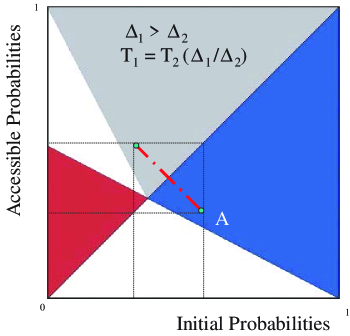
Figure 4: For the cavity in contact with a heat sink at $T_{2}$ where we want the initial probability to be lowered upon leaving, the accessible leaving probability is bounded in the (blue) area under the diagonal, with its reflection shown in gray above the diagonal. The bounded (red) area above the diagonal is for the cavity in contact with a heat bath at $T_{1}=T_{2}(\Delta_{1}/\Delta_{2})$. The reflection of the point A at $T_{2}$ across the diagonal is clearly not in the accessible region at $T_{1}$, as there is no overlapping of the two regions above the diagonal. So we cannot form a cyclic quantum heat engine which does work at these temperatures, even when $T_{1}$ is greater than $T_{2}$ by a factor $(\Delta_{1}/\Delta_{2})$.

For the cavity in contact with the heat bath at $T_{1}$, we want to have the exit probability to be greater (the greater, the more work can be extracted) than the initial probability,

$$p_{u}^{\,(1)}(\tau_{1}) > p_{u}^{\,(1)}(0)=p_{u}^{\,(2)}(\tau_{2}),$$ (28)

thus we need only to consider the appropriate portion of the bounds for this cavity, namely that above the diagonal. Reversely, for the cavity in contact with the heat bath at $T_{2}$, we want to have the exit probability to be smaller (the smaller, the better) than the initial probability,

$$p_{u}^{\,(2)}(\tau_{2}) < p_{u}^{\,(2)}(0)=p_{u}^{\,(1)}(\tau_{1}),$$ (29)

hence for this cavity we need only to consider the other portion of the bounds below the diagonal. Thus, we can also use this Figure 4 to elucidate the situation for the two heat baths in which $T_{1}=T_{2}(\Delta_{1}/\Delta_{2})$, the (red) area above the diagonal comes from $T_{1}$ and the (blue) below the diagonal from $T_{2}$. The coordinate of a point $A$ in the (blue) area below the diagonal in Fig. 4 is $(p_{u}^{\,(2)}(0),p_{u}^{\,(2)}(\tau_{2}))$, representing an exit probability less than the entry one at the cavity with temperature $T_{2}$. The corresponding point at temperature $T_{1}$ must have, by requirement of cyclicity, the coordinate

$$(p_{u}^{\,(1)}(0),p_{u}^{\,(1)}(\tau_{1})) = (p_{u}^{\,(2)}(\tau_{2}),p_{u}^{\,(2)}(0)),$$ (30)

which thus is the reflection of the point $A$ across the diagonal. The gray area above the diagonal in Fig. 4 is the reflection of the (blue) area for $T_{2}$. However, it is clearly seen that for $T_{1}=T_{2}(\Delta_{1}/\Delta_{2})$ this reflection is not in the accessible (red) area for $T_{1}$. We then conclude that at these temperatures, even with $T_{1}$ greater than $T_{2}$ by a factor $(\Delta_{1}/\Delta_{2})$, the quantum heat engines cannot do work on the average. As a consequence of the temperature-independent efficiency similar to (9), the engines cannot neither absorb nor transfer any heat.

In Fig. 5, we combine the relevant bounds for $T_{2}$ below the diagonal (in blue) and those for $T_{1}$ above the diagonal (in red) for the choice $T_{1}<T_{2}(\Delta_{1}/\Delta_{2})$. It is seen once again that no work is derivable on the average. Not only we have thus confirmed the second law that, on the average, no process is possible whose sole result is the transfer of heat from a cooler to a hotter body, with or without a production of work. But we have also clarified the degrees of coolness and hotness in terms of the quantum energy gaps involved before such a process is possible; namely, we must have $T_{1}>T_{2}(\Delta_{1}/\Delta_{2})$, as in (7) once again.

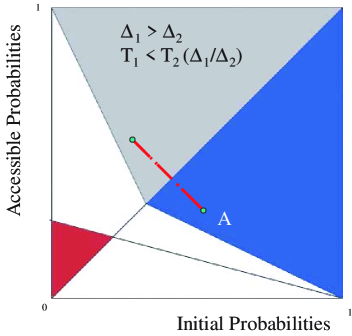
Figure 5: Similar to Fig. 4 but this time with $T_{1}<T_{2}(\Delta_{1}/\Delta_{2})$. Once again we cannot have a cyclic quantum heat engine, even for $T_{1}$ in the range $T_{2}<T_{1}<T_{2}(\Delta_{1}/\Delta_{2})$.

We now show how our quantum heat engines are capable of performing more work than can be derived from thermal equilibrium otherwise. In Fig. 6, which combines the case $T_{1}>T_{2}(\Delta_{1}/\Delta_{2})$, there is some overlap between the (red) area for $T_{1}$ and the reflection of the area for $T_{2}$ across the diagonal. In this case, it can be seen that the production of some work, $\Delta W_{\rm cav}$, is now possible,

$$\left|\Delta W_{\rm cav}\right| = \left(p_{u}^{\,(1)}(\tau_{1})-p_{u}^{\,(2)}(\tau_{2})\right)\left(\Delta_{1}-\Delta_{2}\right).$$ (31)

In general, if and when we choose to operate with a point below the thermal equilibrium line in the (blue) area for $T_{2}$ such that its reflection across the diagonal is above the thermal equilibrium line in the (red) area for $T_{1}$ as shown in the figure, we can derive more work than the case of thermal equilibrium. The work done is proportional to the difference in probabilities as shown in (4) and (31). Here $\left|\Delta W_{\rm cav}\right|$ is greater than the work derivable at thermal equilibrium, $\left|\Delta W_{\rm th}\right|$, because the vertical distance between point $A$ and its reflection in Fig. 6 is greater than the vertical distance between the two horizontal lines, which represent the two thermal equilibria.

From the bounds (25) and (27), we can evaluate the maximum amount of work extractable from our modified quantum heat engines at given temperatures

$$\frac{\max\left|\Delta W_{\rm cav}\right|}{\left|\Delta W_{\rm th}\right|} = \frac{\left(1+2\bar{n}_{1}\right)\left(1+2\bar{n}_{2}\right)}{\left(1+\bar{n}_{1}+\bar{n}_{2}\right)}>1.$$ (32)

Figure 6: Similar to Fig. 4 but this time with $T_{1}>T_{2}(\Delta_{1}/\Delta_{2})>T_{2}$. We can form a cyclic quantum heat engine at these temperatures, in broad agreement with the classical statement of second law. The maximum work that can be extracted in a single cycle is proportional to the length of the (yellow) vertical double arrow and is more than that for thermally equilibrated situation, which is proportional to the distance between the two horizontal (green) lines which represent the thermal equilibrium probabilities for these $T_{1}$ and $T_{2}$ respectively.

VIII An illustration

As an illustration that we can choose and a priori fix the time $\tau_{1}$ and $\tau_{2}$ for all the cycles of the modified mode of operation for our quantum heat engines such that more work can be derived than otherwise available from thermal equilibrium, we present herein the example in Figs. 7 and 8. These numerical results are obtained from (22) with $g=1$ and other parameters as stated in the captions. Note that in Fig. 7 the probability at subsequent time is always more than that of the initial time, in agreement with the fact that the (red) area for $T_{1}$ is above the diagonal in Fig. 6. The reverse is true for Fig. 8, because the (blue) area for $T_{2}$ is below the diagonal in Fig. 6.

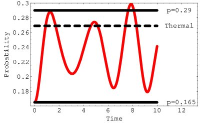
Figure 7: $p_{u}^{\,(1)}$ versus time according to eq. (22). The system enters a single-mode cavity, in contact with a heat source at temperature $T_{1}$ (here, $kT_{1}/\Delta_{1}=1.5$), with the probability in the upper state $p_{u}^{\,(1)}(0)=0.165$ ($=p_{u}^{\,(2)}(\tau_{2})$, by cyclicity requirement) and leaves the cavity, at suitably chosen time $\tau_{1}$, with the increased probability $p_{u}^{\,(1)}(\tau_{1})=0.29$. This latter probability is larger than the thermal equilibrium probability at this temperature (dashed line).

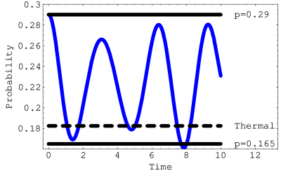
Figure 8: $p_{u}^{\,(2)}$ versus time. Similar to Fig. 7 but this time the probability upon entering a cavity, in contact with a heat sink at temperature $T_{2}<T_{1}(\Delta_{2}/\Delta_{1})<T_{1}$ (here, $kT_{2}/\Delta_{2}=1.0$), is $p_{u}^{\,(2)}(0)=0.29$ ($=p_{u}^{\,(1)}(\tau_{1})$, by cyclicity requirement) and upon leaving, at suitably chosen time $\tau_{2}$, is $p_{u}^{\,(2)}(\tau_{2})=0.165$, completing a cycle of the quantum heat engine. The latter probability is lower than the thermal equilibrium probability at this temperature (dashed line), thus allowing more work to be extracted.

IX Maxwell’s daemon revisited

The expression (22) for the probability, derived from (19), requires some careful justifications. Following Scully and Zubairy (1997), we expand the state vector $|\psi\rangle$ (dropping the superscript $(i)$) in terms of $|u,n\rangle$, in which the engine is in the upper state $|u\rangle$ and the field has exactly $n$ photons, and of $|l,n\rangle$ in which the engine is in the lower state $|l\rangle$,

$$|\psi\rangle = \sum_{n}\left(c_{u,n}(t)|u,n\rangle+c_{l,n}(t)|l,n\rangle\right).$$ (33)

From this, the Schrödinger equation (21) can now be replaced by

$$\dot{c}_{u,n} = -ig\sqrt{n+1}\,c_{l,n+1},$$

$$\dot{c}_{l,n+1} = -ig\sqrt{n+1}\,c_{u,n}.$$ (34)

The general solutions for these probability amplitudes are

$$c_{u,n}(t) = c_{u,n}(0)\cos\left(\Omega_{n}t\right)-ic_{l,n+1}(0)\sin(\Omega_{n}t),$$

$$c_{l,n+1}(t) = c_{l,n+1}(0)\cos(\Omega_{n}t)-ic_{u,n}(0)\sin(\Omega_{n}t),$$ (35)

in which the initial probability amplitudes are assumed to be factorised,

$$c_{u,n}(0) = \sqrt{p_{u}(0)}\times\sqrt{P_{n}},$$

$$c_{l,n+1}(0) = e^{i\theta_{s}}\sqrt{1-p_{u}(0)}\times e^{i\theta_{f}}\sqrt{P_{n+1}},$$ (36)

where the relative phases $\theta_{s}$ for the engine and $\theta_{f}$ for the field, respectively, are not zero in general.

Now, we can also express the probability on the lhs of (22) as

$$p_{u}(t) = \sum_{n}|c_{u,n}(t)|^{2}.$$ (37)

Direct substitution of the amplitudes above, however, leads an additional cross term which does not exist on the rhs of expression (22) but is proportional to

$$\sim\Re\left(ie^{i\theta_{s}}\sqrt{p_{u}(0)\left(1-p_{u}(0)\right)}\times\sum_{n}e^{i\theta_{f}}\sqrt{P_{n}P_{n+1}}\,\cos\left(\Omega_{n}t\right)\sin\left(\Omega_{n}t\right)\right).$$ (38)

Accordingly, the various bounds for $p_{u}(t)$ will be modified by the term $\sqrt{p_{u}(0)\left(1-p_{u}(0)\right)}$, which is nonlinear in $p_{u}(0)$, unlike the situation in (25, 27) depicted in Fig. 4, from which the second law was seen to be followed. One might think that this extra non-linear term could be exploited to beat the second law (thanks to the newly emerged overlapping of regions which were not overlapped previously in Fig. 4). But this is not meant to be, however. The reason for this impossibility is that, in general, the various phases in (38) are not fixed but can be random, especially for the phase $\theta_{f}$ of the thermal field. They will have to be averaged over, rendering the cross term (38) vanished after all. We thus get back the expression (22) exactly.

If the phases could be controlled physically then the second law might be violated. But the point to be emphasised here is that such a control of the phases will require some careful operation which is nothing more than just another disguised act of Maxwell’s daemon. In the end, any such resulted violation of the second law, if possible, is not and should not be surprising at all.

X Quantum heat engines with 1-D simple harmonic oscillators

We now generalise some of the above results to quantum systems having an infinite number of energy levels. Firstly, we consider a 1-D simple harmonic oscillator of frequency $\omega_{1}$ in thermal equilibrium with a heat bath at $T_{1}$. The oscillator is then removed from the heat bath to undergo a quantum adiabatic expansion until its frequency is dropped to $\omega_{2}$. It is then equilibrated with another heat bath at temperature $T_{2}$ before undergone another quantum adiabatic compression to raise its frequency back to $\omega_{1}$. In one such cycle, the oscillator performs an amount of work,

$$\Delta W = \sum_{n=0}^{\infty}\left(E_{n}^{\,(1)}-E_{n}^{\,(2)}\right)\left(p_{n}^{\,(2)}-p_{n}^{\,(1)}\right),$$ (39)

$$= \hbar\left(\omega_{1}-\omega_{2}\right)\sum_{n=0}^{\infty}\left(n+\frac{1}{2}\right)\left(p_{n}^{\,(2)}-p_{n}^{\,(1)}\right),$$

$$= \hbar\left(\omega_{1}-\omega_{2}\right)\sum_{n=0}^{\infty}n\left(p_{n}^{\,(2)}-p_{n}^{\,(1)}\right),$$

with the Gibbs distributions for $i=1,2$

$$p_{n}^{\,(i)} = \left(1-e^{-\alpha_{i}}\right)e^{-n\alpha_{i}},$$ (40)

and

$$\alpha_{i} = \frac{\hbar\omega_{i}}{kT_{i}}.$$ (41)

We have used the energy expressions for simple harmonic oscillators

$$E_{n}^{\,(i)} = \left(n+\frac{1}{2}\right)\hbar\omega_{i}.$$ (42)

Let

$$x=\alpha_{2}-\alpha_{1}$$ (43)

and consider the sum in (39) as a function of $x$,

$$f(x) = \sum_{n=0}^{\infty}n\left\{\left(1-e^{-\alpha_{1}-x}\right)e^{-n\alpha_{1}-nx}-\left(1-e^{-\alpha_{1}}\right)e^{-n\alpha_{1}}\right\}.$$ (44)

Its derivative is

$$f^{\prime}(x) = -\sum_{m=1}^{\infty}me^{-m\left(\alpha_{1}+x\right)},$$ (45)

which is always negative (we always have $x>-\alpha_{1}$ for the convergence of the infinite sum, as $\alpha_{2}>0$). Thus $f(x)$ is a monotonically decreasing function; in particular, $f(x)<f(0)=0$ for $x\geq 0$. From the definition of $x$ (43) and $f(x)$ (44) we conclude that the oscillator can only perform work on the environment (i.e. when $f(x)<0$) if and only if $x>0$, which means that $\alpha_{2}>\alpha_{1}$. That is,

$$T_{1} > T_{2}\left(\frac{\omega_{1}}{\omega_{2}}\right)$$ (46)

is the necessary and sufficient condition for work to be performed by a quantum simple harmonic oscillator in such a cycle described above.

XI Quantum heat engines with 1-D infinite square wells

Similarly to the last Section, but we now replace the oscillator by a particle of mass $m$ in an 1-D infinite square well. The work performed in a cycle is also

$$\Delta W = \sum_{n=0}^{\infty}\left(E_{n}^{\,(1)}-E_{n}^{\,(2)}\right)\left(p_{n}^{\,(2)}-p_{n}^{\,(1)}\right),$$ (47)

but this time with the energies

$$E_{n}^{\,(i)} = n^{2}\frac{\hbar^{2}\pi^{2}}{2mL^{2}_{i}}$$ (48)

and the thermal distributions

$$p_{n}^{\,(i)} = \frac{e^{-\beta_{i}E_{n}^{\,(i)}}}{\sum_{m}e^{-\beta_{i}E_{m}^{\,(i)}}},$$ (49)

where $\beta_{i}=1/(kT_{i})$ and $L_{i}$ are the widths of the wells at $T_{i}$.

Let

$$y = \beta_{2}-\beta_{1},$$ (50)

and consider the rhs of (47) as a function $g$ of $y$. Its derivative wrt $y$ can be written as

$$g^{\prime}(y) = \langle E^{(2)}(E^{(1)}-E^{(2)})\rangle_{y}+\langle E^{(1)}-E^{(2)}\rangle_{y}\langle E^{(2)}\rangle_{y},$$ (51)

where

$$\langle O\rangle_{y} \equiv \sum_{n}O_{n}p_{n}^{\,(2)},$$ (52)

note that $p_{n}^{(2)}$ is a function of $y$.

Substituting the energy expressions (48) into the derivative (51), with $L_{2}>L_{1}$,

$$g^{\prime}(y) = \left(\langle n^{4}\rangle_{y}-\langle n^{2}\rangle_{y}^{2}\right)\frac{\hbar^{2}\pi^{2}}{2mL^{2}_{2}}\left(\frac{\hbar^{2}\pi^{2}}{2mL^{2}_{2}}-\frac{\hbar^{2}\pi^{2}}{2mL^{2}_{1}}\right),$$ (53)

which is not positive, but can vanish, thanks to the well-known positivity property of the expression in the first pair of curly parentheses. Noting that $g(0)=0$, we have $\Delta W=g(y)>g(0)=0$ if and only if $y<0$; that is if and only if

$$T_{1} < T_{2}.$$ (54)

This is the condition upon which the system cannot do work and and which is in accordance with the second law of thermodynamics.

Note also that the above mathematical derivation can also be applied to the simple harmonic oscillators of Section X once we replace the energy expressions (48) by those of (42). However, the ability to exactly evaluate the partition functions of the simple harmonic oscillators of Section X enables us to derive the condition (46), which is not contradictory to but has a more positive interpretation than the condition (54) above: even though $\Delta W=g(y)\leq 0$ if and only if $y\geq 0$, we cannot conclude, because of the possibility that $g(y)$ can vanish, that the system can do work if $T_{1}\geq T_{2}$. This thus is consistent with (46), which is the condition whence work can be extracted.

XII Concluding remarks

By interpreting work and heat, but without referring to entropy directly, in the quantum domain and by applying this interpretation to the simplest quantum systems, we have not only confirmed the broad validity of the second law but also been able to clarify and refine its various aspects. On the one hand, explicitly because of the probabilistic nature of quantum mechanics, there do exist physical processes which can violate certain classical statements of the second law. However, such violation only occurs randomly and thus it cannot be exploitable nor harnessible. On the other hand, the second law is seen to be valid on the average. This confirmation of the second law is in accordance with the fact that, while we can treat the quantum heat engines purely and entirely as quantum mechanical systems, we still have to assume the Gibbs distributions for the heat baths involved. Such distributions can only be derived Landau et al. (1980) with non-quantum-mechanical assumptions, which ignore, for example, any quantum entanglement within the heat baths. Indeed, it has been shown that Lenard (1978); Tasaki (2000) the law of entropy increase is a mathematical consequence of the initial states being in such general equilibrium distributions. This illustrates and highlights the connection between the second law to the unsolved problems of emergence of classicality, of quantum measurement and of decoherence which are inter-related and central to quantum mechanics. Only until some further progress is made on these problems, the classicality of the heat baths will have to be assumed and remained hidden in the assumption of the Maxwell-Boltzmann-Gibbs thermal equilibrium distributions.

Even our results support the second law, on the average, we have further clarified the degree of temperature difference (7), in terms of the quantum energy gaps involved, between the heat baths before any work can be extracted. While the Carnot efficiency is an upper bound for that of the quantum heat engines, the former could be approached by the quantum engines with the introduction of an infinite number of alternating adiabatic and heat transferred steps. The implication of this approach in the context of quantum information deserves further investigations elsewhere.

Inspired and motivated by the Rabi oscillations, we have also shown how to extract more work from the heat baths than otherwise possible with thermal equilibrium distributions – but more heat input would also be needed in such a way that the Carnot efficiency is still a valid upper bound. Note that such an operation is subject to the bounds given in (25) and (27), which then, as can be seen through their depiction in the figures, ensure that we stay within the second law, but refined with the necessary condition (7). The perfect agreement between the specific results derived from the quantum dynamical bounds (25) and (27) with the general result (7) derived from statistical mechanics is quite remarkable. We speculate that such agreement is not accidental but is a consequence of the Gibbs distributions assumed for the heat baths in both derivations; and the agreement should thus be independent of specific details of the quantum dynamics involved. Note also that the modified operation with single-mode cavities is not an operation of Maxwell’s daemon because the information about the time intervals $\tau_{1}$ and $\tau_{2}$ is fixed and forms an integrated part of the modified engines. This information, being common to all cycles, need not and should not be erased after each cycle to preserve the cyclicity condition. Other studies of very different classes of quantum heat engines Scully et al. (2003); Maruyama et al. (2005) have apparently claimed similar results that more work can be derived than from classical engines. (However, if the cyclicity condition is not strictly observed for a heat engine, as in the case for some of those studies, then some extra effects may be hidden or unaccounted for, such as those associated with a maintenance of some coherent states or some Fock state, and apparent violation of the second law might thus be possible.)

Our class of quantum heat engines can also readily offer a feasible way to physically realise Maxwell’s daemon, in a way different to Szilard’s engine but also through the acts of quantum measurement and information erasure. Finally, some of our results above have also been generalised to quantum heat engines having an infinite number of energy levels, specifically the 1-D simple harmonic oscillators and 1-D infinite square wells. Some analysis of three-level quantum heat engines has also been available recently Quan et al. (2005), but because of the many different energy gaps available (similar to the case of square well), different conditions with different combinations of gap ratios could enter a counterpart of (4) above.