Analytic solutions for quantum logic gates and modeling pulse errors in a quantum computer with a Heisenberg interaction

Abstract

We analyze analytically and numerically quantum logic gates in a one-dimensional spin chain with Heisenberg interaction. Analytic solutions for basic one-qubit gates and swap gate are obtained for a quantum computer based on logical qubits. We calculated the errors caused by imperfect pulses which implement the quantum logic gates. It is numerically demonstrated that the probability error is proportional to $\varepsilon^{4}$, while the phase error is proportional to $\varepsilon$, where $\varepsilon$ is the characteristic deviation from the perfect pulse duration.

I Introduction

It is known that the Heisenberg interaction alone can provide a universal set of gates for quantum computation DNature . A computer based on the Heisenberg interaction does not require magnetic fields nor electromagnetic pulses. Implementations of a quantum computer using the Heisenberg interaction between the spins of the quantum dots or impurities in semiconductors promise clock-speeds in GHz region. The spins do not interact with each other unless one applies a voltage, which turns on the exchange interaction between a selected pair of spins.

In order to perform single-qubit rotations using the Heisenberg interaction, one should use coded, or logical, qubits. In this paper, we use the coding introduced in Ref. DNature and derive optimal gate sequences to implement swap gate and basic one-qubit logic operations. The errors caused by imperfections of the pulses are investigated numerically. The random deviations in the areas of the pulses in our simulations are assumed to have a Gaussian distribution with variance $\varepsilon$.

II Quantum dynamics

Consider the dynamics of a spin system with an isotropic Heisenberg interaction between neighboring spins. The Hamiltonian which describes the interaction $J(\bar{t})$ between $k$th and $(k+1)$th spins is

$$H_{k}(\bar{t})=J(\bar{t}){\rm\bf S}_{k}{\rm\bf S}_{k+1},$$ (1)

where $\bar{t}$ is time, ${\rm\bf S}_{k}$ is the operator of the $k$th spin $1/2$. The solution of the Schrödinger equation with the Hamiltonian (1) can be written in the form

$$\psi(\bar{t})=\exp\left(-{i\over\hbar}\int_{0}^{\bar{t}}J(\bar{t}^{\prime})d\bar{t}^{\prime}{\rm\bf S}_{k}{\rm\bf S}_{k+1}\right)\psi(0).$$ (2)

(We do not use the time-ordering operator because $[H_{k}(\bar{t}),H_{k}(\bar{t}^{\prime})]=0$.) Introducing a new effective dimensionless time,

$$t={1\over 2\pi\hbar}\int_{0}^{\bar{t}}J(\bar{t}^{\prime})d\bar{t}^{\prime},$$ (3)

one can write Eq. (2) as

$$\psi(t)=\exp\left(-i2\pi t{\rm\bf S}_{k}{\rm\bf S}_{k+1}\right)\psi(0).$$ (4)

This is the solution of the following dimensionless Schrödinger equation:

$$i{\partial\psi(t)\over\partial t}=V_{k}\psi(t),$$ (5)

where

$$V_{k}=2\pi\left[S_{k}^{z}S_{k+1}^{z}+\frac{1}{2}(S_{k}^{+}S_{k+1}^{-}+S_{k}^{-}S_{k+1}^{+})\right]$$ (6)

is the dimensionless Hamiltonian, $S_{k}^{x}$ $S_{k}^{y}$, and $S_{k}^{z}$ are the components of the operator ${\rm\bf S}_{k}$, $S_{k}^{\pm}=S_{k}^{x}\pm iS_{k}^{y}$. After decomposition of the wave function in the basis states $|n\rangle$,

$$\psi(t)=\sum_{n}C_{n}(t)|n\rangle,$$ (7)

where the states $|n\rangle$ are defined below in Eqs. (11) and (46), one obtains a system of dimensionless differential equations for the expansion coefficients,

$$i\dot{C}_{n}=\sum_{m}\langle n|V_{k}|m\rangle C_{m},$$ (8)

where the dot indicates differentiation with respect to time $t$.

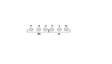
Figure 1: Coding two logical qubits using six physical qubits.

The matrix elements in Eq. (8) can be calculated by action of the Hamiltonian $V_{k}$ in Eq. (6) on the physical qubits (spins) using the following relations:

$$S_{k}^{z}|\dots 0_{k}\dots\rangle=\frac{1}{2}|\dots 0_{k}\dots\rangle,\qquad S_{k}^{z}|\dots 1_{k}\dots\rangle=-\frac{1}{2}|\dots 1_{k}\dots\rangle,$$

$$S_{k}^{+}|\dots 0_{k}\dots\rangle=0,~{}~{}\qquad S_{k}^{+}|\dots 1_{k}\dots\rangle=|\dots 0_{k}\dots\rangle,$$ (9)

$$S_{k}^{-}|\dots 0_{k}\dots\rangle=|\dots 1_{k}\dots\rangle,\qquad S_{k}^{-}|\dots 1_{k}\dots\rangle=0.~{}$$

III Single qubit gates

Let us consider only the first three spins, 0, 1, and 2, of the spin chain in Fig. 1. We suppose that initially there are two spins in the state $|0\rangle$ and one spin in the state $|1\rangle$. Since the Hamiltonians $V_{k}$ can not flip individual spins (but can only swap the neighboring spins) one can choose an invariant subspace spanned by only three states of the $2^{3}=8$ basis states:

$$|0_{2}0_{1}1_{0}\rangle,~{}~{}~{}|0_{2}1_{1}0_{0}\rangle,~{}~{}~{}|1_{2}0_{1}0_{0}\rangle,$$ (10)

or by their normalized and orthogonal superpositions DNature ,

$$|0\rangle=|0_{\rm A}\rangle={1\over\sqrt{2}}(|0_{2}1_{1}0_{0}\rangle-|1_{2}0_{1}0_{0}\rangle),~{}~{}|1\rangle=|1_{\rm A}\rangle=\sqrt{{2\over 3}}\left(|0_{2}0_{1}1_{0}\rangle-{1\over 2}|0_{2}1_{1}0_{0}\rangle-{1\over 2}|1_{2}0_{1}0_{0}\rangle\right),$$

$$|2\rangle=|a_{\rm A}\rangle={1\over\sqrt{3}}\left(|0_{2}0_{1}1_{0}\rangle+|0_{2}1_{1}0_{0}\rangle+|1_{2}0_{1}0_{0}\rangle\right).$$ (11)

We define the state $|0_{\rm A}\rangle$ as the ground state of the logical qubit A; the state $|1_{\rm A}\rangle$ as the excited state; and the state $|a_{\rm A}\rangle$ as the auxiliary state. One can show that all matrix elements for transitions to the state $|a_{\rm A}\rangle$ are equal to zero,

$$\langle a_{A}|V_{0}|0_{A}\rangle=\langle a_{A}|V_{0}|1_{A}\rangle=\langle a_{A}|V_{1}|0_{A}\rangle=\langle a_{A}|V_{1}|1_{A}\rangle=0.$$ (12)

If the state $|a_{\rm A}\rangle$ is initially not populated, it remains empty under the action of the Hamiltonians $V_{0}$ and $V_{1}$. For the single-qubit operations, analyzed in this Section we assume that initially $C_{2}(t=0)=0$ and we consider the dynamics including only the states $|0\rangle=|0_{A}\rangle$ and $|1\rangle=|1_{A}\rangle$.

The matrix elements of the two Hamiltonians have the form

$$V_{0}:~{}\pmatrix{0&-\Omega/2\cr-\Omega/2&\Delta},\qquad V_{1}:~{}\pmatrix{3\Delta/2&0\cr 0&-\Delta/2},$$ (13)

where

$$\Delta=-\pi,\qquad\Omega=-\sqrt{3}\pi.$$ (14)

The solution of the Schrödinger equation generated by the diagonal matrix $V_{1}$ has the form

$$C_{0}(t)=e^{-i3\Delta t/2}C_{0}(0),\qquad C_{1}(t)=e^{i\Delta t/2}C_{1}(0).$$ (15)

The solution generated by the matrix $V_{0}$ is

$$C_{0}(t)=\left\{C_{0}(0)\left[\cos(\Lambda t/2)+i{\Delta\over\Lambda}\sin(\Lambda t/2)\right]+iC_{1}(0){\Omega\over\Lambda}\sin(\Lambda t/2)\right\}e^{-i\Delta t/2},$$

$$C_{1}(t)=\left\{C_{1}(0)\left[\cos(\Lambda t/2)-i{\Delta\over\Lambda}\sin(\Lambda t/2)\right]+iC_{0}(0){\Omega\over\Lambda}\sin(\Lambda t/2)\right\}e^{-i\Delta t/2},$$ (16)

where

$$\Lambda=\sqrt{\Delta^{2}+\Omega^{2}}=2\pi.$$ (17)

For convenience, we present below all dependences expressed in terms of the frequencies $\Omega$, $\Delta$, and $\Lambda$, but not in terms of their numerical values.

III.1 One logical qubit flip

In order to flip the logical qubit A using Eq. (16) we assume

$$C_{0}(0)=1,~{}~{}C_{1}(0)=0,$$ (18)

and apply the Hamiltonian $V_{0}$ for time $t$. Then, one obtains

$$C_{0}(t)=\left[\cos(\Lambda t/2)+i{\Delta\over\Lambda}\sin(\Lambda t/2)\right]e^{-i\Delta t/2},$$

$$C_{1}(t)=i{\Omega\over\Lambda}\sin(\Lambda t/2)e^{-i\Delta t/2}.$$ (19)

From this solution one can see that it is impossible to flip the logical qubit using only one pulse since the coefficient $C_{0}(t)$ in Eq. (19) does not become zero for any $t$. To solve this problem we use the pulse sequence

$${\rm F}_{\rm A}^{\rm ph}=V_{0}(t_{3})V_{1}(t_{2})V_{0}(t_{1}),$$ (20)

proposed in Ref. DNature . Here and below the superscript ‘ph’ indicates that the gate requires additional pulses to implement the phase correction. In Eq. (20) $V_{i}(t)$ indicates action of $i$th Hamiltonian during time $t$, and the sequence must be read from right to left. In this Section we obtain exact analytical expressions for $t_{1}$, $t_{2}$, and $t_{3}$.

A flip of the qubit A with the initial conditions (18) means making the transition $|0\rangle\rightarrow|1\rangle$. Using Eqs. (15), (16), and (18) and setting the amplitude $C_{0}(t)=0$ after the action of the ${\rm F}^{\rm ph}_{\rm A}$ gate, one obtains the equation

$$e^{-i{\Delta\over 2}(t_{1}-t_{2}+t_{3})}\left\{e^{-2i\Delta t_{2}}\left[\cos(\Lambda t_{1}/2)+i{\Delta\over\Lambda}\sin(\Lambda t_{1}/2)\right]\left[\cos(\Lambda t_{3}/2)+i{\Delta\over\Lambda}\sin(\Lambda t_{3}/2)\right]-\right.$$

$$\left.{\Omega^{2}\over\Lambda^{2}}\sin(\Lambda t_{1}/2)\sin(\Lambda t_{3}/2)\right\}=0.$$ (21)

Equation (21) is satisfied when both the real and the imaginary parts of the expression in the curly brackets are equal to zero.

In order to solve Eq. (21) we first assume that $\cos(\Lambda t_{1}/2)\neq 0$, $\cos(2\Delta t_{2})\neq 0$, and $\cos(\Lambda t_{3}/2)\neq 0$. Then, for

$$x=\tan(\Lambda t_{1}/2),~{}~{}y=\tan(2\Delta t_{2}),~{}~{}z=\tan(\Lambda t_{3}/2)$$

one obtains the following system of two coupled equations:

$$1-xz+{\Delta\over\Lambda}y(x+z)=0,$$

$$y\left(1-{\Delta^{2}\over\Lambda^{2}}xz\right)+{\Delta\over\Lambda}(x+z)=0.$$ (22)

Using Eqs. (14) and (17) and eliminating $y$, one has

$$(xz-1)(4-xz)=(x+z)^{2}.$$ (23)

Introducing the notations $x+z=2b$ and $xz=c$ one can present $x$ and $z$ as the two solutions ($\xi_{1}=x$ and $\xi_{2}=z$) of the quadratic equation

$$\xi^{2}-2b\xi+c=0.$$ (24)

Using definitions of $b$ and $c$ and Eq. (23) one can show that Eq. (24) has no real solution.

In a similar way one can show that there is no real solution when $\cos(\Lambda t_{1}/2)=0$ or $\cos(\Lambda t_{3}/2)=0$. For $\cos(2\Delta t_{2})=0$, the two solutions are

$${t^{\prime}}_{1}={{\rm arctan}(3-\sqrt{5})\over\pi},~{}~{}{t^{\prime}}_{2}=\frac{1}{4},~{}~{}{t^{\prime}}_{3}={{\rm arctan}(3+\sqrt{5})\over\pi}$$

and

$$t_{1}=1-{{\rm arctan}(3-\sqrt{5})\over\pi},~{}~{}t_{2}=\frac{3}{4},~{}~{}t_{3}=1-{{\rm arctan}(3+\sqrt{5})\over\pi}.$$ (25)

Below we use only the second solution (25).

The ${\rm F}_{\rm A}^{\rm ph}$ gate generates different phases for two basis states,

$${\rm F}_{\rm A}^{\rm ph}\pmatrix{C_{0}\cr C_{1}}=\pmatrix{e^{i\varphi_{2}}C_{1}\cr e^{i\varphi_{1}}C_{0}},$$ (26)

where

$$\varphi_{1}=\frac{1}{2}\left[\frac{3\pi}{4}+{\rm arctan}~{}2-{\rm arctan}(\sqrt{5}/2)\right],~{}~{}~{}\varphi_{2}=\frac{1}{2}\left[\frac{3\pi}{4}+{\rm arctan}~{}2+{\rm arctan}(\sqrt{5}/2)\right].$$ (27)

In order to correct the phases, an additional pulse is required. The phase-corrected gate ${\rm F}_{\rm A}$ for flipping the qubit A has the form

$${\rm F}_{\rm A}=V_{1}(t_{4})F_{\rm A}^{\rm ph}=V_{1}(t_{4})V_{0}(t_{3})V_{1}(t_{2})V_{0}(t_{1}).$$ (28)

In order to find the time $t_{4}$ we use the solution (15). The additional phase-correcting pulse $V_{1}(t_{4})$ modifies Eq. (26) to become

$${\rm F}_{\rm A}\pmatrix{C_{0}\cr C_{1}}=\pmatrix{e^{i(\varphi_{2}-3\Delta t_{4}/2)}C_{1}\cr e^{i(\varphi_{1}+\Delta t_{4}/2)}C_{0}}.$$ (29)

One can make the phases of the both states equal to each other by application of the ${\rm F}_{\rm A}$ gate if the condition

$$\varphi_{1}+\Delta t_{4}/2=\varphi_{2}-3\Delta t_{4}/2$$

is satisfied. This equation determines the last parameter,

$$t_{4}=1-{{\rm arctan(\sqrt{5}/2)}\over 2\pi},$$ (30)

required to implement the phase-corrected flip of the qubit A. The flip gate for the qubit A can be written as

$${\rm F}_{\rm A}\pmatrix{C_{0}\cr C_{1}}=e^{i\Phi_{\rm F}}\pmatrix{C_{1}\cr C_{0}},$$ (31)

where the overall phase for the single qubit flip gate is

$$\Phi_{\rm F}=-{\pi\over 8}+{1\over 2}\,{\rm arctan}~{}2-{1\over 4}\,{\rm arctan(\sqrt{5}/2)}.$$ (32)

III.2 Hadamard transform

The Hadamard transform H_A for the qubit A can be performed using the pulse sequence

$${\rm H}_{\rm A}=V_{1}(t_{5})V_{0}(t_{6})V_{1}(t_{5}).$$ (33)

Here the pulses $V_{1}(t_{5})$ are used to provide the correct phases and the pulse $V_{0}(t_{6})$ is needed to split each of the states $|0\rangle$ and $|1\rangle$ into a superposition of the states with equal probabilities. The time-intervals are

$$t_{5}=\frac{3}{4}+{{\rm arctan}(1/\sqrt{2})\over 2\pi},\qquad t_{6}={{\rm arctan}\sqrt{2}\over\pi}.$$ (34)

The Hadamard gate transforms the wave function as

$${\rm H}_{\rm A}\pmatrix{C_{0}\cr C_{1}}={e^{i\pi/2}\over\sqrt{2}}\pmatrix{C_{0}+C_{1}\cr C_{0}-C_{1}}.$$ (35)

III.3 Phase gate

The phase gate P${}_{\rm A}(\theta)$ for the qubit A can be performed using only one pulse

$${\rm P}_{\rm A}(\theta)=V_{1}[t(\theta)],$$ (36)

where

$$t(\theta)=1-{\theta\over 2\pi},$$ (37)

and the angle $\theta$ is defined in the interval $[0,2\pi]$. The Phase gate transforms the wave function in the following way

$${\rm P}_{\rm A}\pmatrix{C_{0}\cr C_{1}}=e^{i\Phi_{\rm P}(\theta)}\pmatrix{C_{0}\cr e^{i\theta}C_{1}}.$$ (38)

The overall phase generated by the phase gate is

$$\Phi_{\rm P}(\theta)={3\pi\over 2}-{3\theta\over 4}.$$ (39)

The single qubit operations for the qubit B in Fig. 1 can be performed using the same sequences like those for the qubit A with the substitutions $V_{0}(t)\rightarrow V_{3}(t)$ and $V_{1}(t)\rightarrow V_{4}(t)$.

IV Swap gate

It is convenient to analyze the spin states [from which the logical qubits are formed, see Eq. (11)]. Consider the four different spin states,

$$|m\rangle=|\dots 0_{k}0_{k+1}\dots\rangle,~{}~{}~{}|p\rangle=|\dots 1_{k}1_{k+1}\dots\rangle,$$

$$|i\rangle=|\dots 1_{k}0_{k+1}\dots\rangle,~{}~{}~{}|j\rangle=|\dots 0_{k}1_{k+1}\dots\rangle.$$ (40)

These states form two one-dimensional and one two-dimensional invariant subspaces. The states $|m\rangle$ and $|p\rangle$ are eigenstates of the Hamiltonian $V_{k}$,

$$V_{k}(t)|m\rangle=e^{-i\frac{\pi}{2}t}|m\rangle,~{}~{}~{}V_{k}(t)|p\rangle=e^{-i\frac{\pi}{2}t}|p\rangle.$$ (41)

The states $|i\rangle$ and $|j\rangle$ are transformed as

$$V_{k}(t)|i\rangle=e^{i\frac{\pi}{2}t}\left[\cos(\pi t)|i\rangle-i\sin(\pi t)|j\rangle\right],$$

$$V_{k}(t)|j\rangle=e^{i\frac{\pi}{2}t}\left[\cos(\pi t)|j\rangle-i\sin(\pi t)|i\rangle\right].$$ (42)

From Eqs. (41) and (42) one can see that the pulse $V_{k}(1/2)$ can be used as a swap gate between the $k$th and $(k+1)$th spins. After the pulse $V_{k}(1/2)$ all states acquire the phase $-i\pi/4$.

The swap gate between the spins can be used for implementation of the swap gate between the logical qubits. The two logical qubits, A and B, in Fig. 1 are formed by the superpositions of the spin states involving six spins. Consider one state of the superposition, for example, the state $|0_{5}0_{4}1_{3}~{}0_{2}1_{1}0_{0}\rangle$. The spins 0, 1, and 2 are related to the logical qubit A and the spins 3, 4, and 5 are related to the logical qubit B. Using five swaps between the neighboring spins one can move the state of the 5th spin to the zeroth spin,

$$C_{5,0}|{\bf 0_{5}}0_{4}1_{3}~{}0_{2}1_{1}0_{0}\rangle=e^{-i{5\pi\over 4}}|0_{5}1_{4}0_{3}~{}1_{2}0_{1}{\bf 0_{0}}\rangle,$$ (43)

where ${\rm C}_{5,0}$ is the operator or the cyclic permutation,

$$C_{5,0}=V_{0}\left(\frac{1}{2}\right)V_{1}\left(\frac{1}{2}\right)V_{2}\left(\frac{1}{2}\right)V_{3}\left(\frac{1}{2}\right)V_{4}\left(\frac{1}{2}\right).$$ (44)

Three successive applications of the operator ${\rm C}_{5,0}$ result in the swap gate S_AB between the logical qubits (below called swap gate),

$${\rm S}_{\rm AB}=C_{5,0}C_{5,0}C_{5,0}.$$ (45)

The swap gate $S_{\rm AB}$ produces an overall phase $\pi/4$ for the wave function. The total number of pulses required to execute the swap gate is 15. Note that the result of the swap gate is independent of a kind of coding of the logical qubits through the spin states.

V Modeling errors in the swap gate

In spite of the rather simple form of the swap gate S_AB, it does implement a complex logic operation on logical qubits. Indeed, if initially one has a basis logical state, e.g. $|1_{\rm B}0_{\rm A}\rangle$, in the process of applying the swap gate one has a superposition of many states, while, finally, only one state ($|0_{\rm B}1_{\rm A}\rangle)$ survives, and all other states disappear.

Numerical simulations of the swap gate between the qubits A and B were performed in the invariant Hilbert subspace spanned by the following 15 [$15=C^{2}_{6}={6!/(2!4!)}$] states:

$$|0\rangle=|0_{\rm B}0_{\rm A}\rangle,~{}~{}|1\rangle=|0_{\rm B}1_{\rm A}\rangle,~{}~{}|2\rangle=|1_{\rm B}0_{\rm A}\rangle,~{}~{}|3\rangle=|1_{\rm B}1_{\rm A}\rangle,~{}~{}$$

$$|4\rangle=|0_{\rm B}a_{\rm A}\rangle,~{}~{}|5\rangle=|1_{\rm B}a_{\rm A}\rangle,~{}~{}|6\rangle=|a_{\rm B}0_{\rm A}\rangle,~{}~{}|7\rangle=|a_{\rm B}1_{\rm A}\rangle,~{}~{}$$

$$|8\rangle=|a_{\rm B}a_{\rm A}\rangle,~{}~{}|9\rangle=|000~{}011\rangle,~{}~{}|10\rangle=|000~{}101\rangle,~{}~{}|11\rangle=|000~{}110\rangle,~{}~{}$$ (46)

$$|12\rangle=|011~{}000\rangle,~{}~{}|13\rangle=|101~{}000\rangle,~{}~{}|14\rangle=|110~{}000\rangle.$$

The dynamics was simulated using the evolution operators built using the eigenstates of the Hamiltonians $V_{k}$, $k=0,1,\dots,5$, in the 15-dimensional space. When the time-intervals $t$ for the pulses were exactly equal to $t=t_{0}=1/2$, the errors in implementation of the swap gate were of the order of $10^{-15}$, i.e. accuracy was limited only by the round-off errors. Since $t$ is proportional to the area of the pulse, the form of the pulse is not important. However, in an experiment there is always some deviation in $t$ from its optimal value $t_{0}$. To understand the error caused by this deviation, we modeled the swap gate with imperfect pulses. The duration of each imperfect pulse is taken as

$$t=t_{0}+\delta t,$$ (47)

where the random deviation $\delta t$ is assumed to have the Gaussian distribution $\exp[-(\delta t)^{2}/(2\varepsilon^{2})]$.

Figure 2: (a) The average probability error $P_{\rm S}$ and (b) the average phase error $Q_{\rm S}$ of the swap gate as a function of $\varepsilon$ (filled circles). The least square fits (solid lines), show that: (a) the probability error increases as $P_{\rm S}=3.183\times 10^{3}\times\varepsilon^{3.998}$, $\chi^{2}=43.5$; (b) the phase error is given by $Q_{\rm S}=10.2033\times\varepsilon^{1.0031}$, $\chi^{2}=1.0$.

We define the probability error as

$$P_{\rm S}=||C_{j}(T)|^{2}-|C_{i}(0)|^{2}|,~{}~{}~{}C_{i}(0)=1,$$ (48)

where $T$ is the duration of the swap gate and the final state $|j\rangle$ is related to the initial state $|i\rangle$ as

$$|j\rangle={\rm S}^{\rm i}_{\rm AB}|i\rangle.$$ (49)

Here ${\rm S}^{\rm i}_{\rm AB}$ is the ideal swap gate. The probability error $P_{\rm S}$, shown in Fig. 2(a), increases as a function of $\varepsilon$ approximately as $3.2\times 10^{3}\times\varepsilon^{4}$.

Next, we study the phase errors [see Fig. 2(b)], caused by the random fluctuation of the pulse duration $t$. Under the action of the sequence (45) of the perfect pulses the four logical basis states $|00\rangle$, $|01\rangle$, $|10\rangle$, and $|11\rangle$ transform correspondingly to $|00\rangle$, $|10\rangle$, $|01\rangle$, and $|11\rangle$ with the same phase shift. Under the action of the imperfect pulses we obtain four different phase shifts for the basis states. We define the phase error $Q_{\rm S}$ as the maximum difference between these phase shifts. From Fig. 2(b) one can see that the phase error is approximately equal to $10.2\varepsilon$.

The data in Figs. 2(a,b) are averaged over 1000 runs with different randomly chosen initial states $|i\rangle$ and different random deviations $\delta t$ from the ideal pulse duration $t_{0}$. In Figs. 2(a,b) $\chi^{2}$ was calculated as chi2

$$\chi^{2}=\sum_{i=1}^{K}{(y_{k}-\bar{y}_{k})^{2}\over(\delta y_{k})^{2}},$$

where the index $k$ labels the points on the graphs, $K$ is the number of points, $y_{k}=P_{\rm S}^{k}$ in Fig. 2(a) and $y_{k}=Q_{\rm S}^{k}$ in Fig. 2(b) are the coordinates of the circles, $\bar{y}_{k}$ are the corresponding coordinates of the points on the straight lines for the same values of $\varepsilon$; $\delta y_{k}$ are the corresponding standard deviations.

VI Conclusion

In this paper, analytic solutions for quantum logic gates are obtained for a quantum computer with an isotropic Heisenberg interaction between neighboring identical spins arranged in a one-dimensional spin chain. Single qubit flip, Hadamard and phase transforms are implemented by using, respectively, 4, 3, and 1 pulse(s). The swap gate is realized using 15 pulses. The probability and phase errors caused by imperfect pulses for the swap gate are calculated numerically. The probability error is proportional to $\varepsilon^{4}$, while the phase error is proportional to $\varepsilon$, where $\varepsilon$ is the characteristic deviation from the perfect pulse duration.

References

• (1) D. P. DiVincenzo, D. Bacon, J. Kempe, G. Burkard, and K. B. Whaley, Nature (London) 408, 339 (2000); quant-ph/0005116 (v2) (2002).
• (2) S.L. Meyer, Data Analysis for Scientists and Engineers (Peer Management Consultants, Ltd., Evanston, 1992).