The density matrix in the de Broglie-Bohm approach

If the density matrix is treated as an objective description of individual systems, it may become possible to attribute the same objective significance to statistical mechanical properties, such as entropy or temperature, as to properties such as mass or energy. It is shown that the de Broglie-Bohm interpretation of quantum theory can be consistently applied to density matrices as a description of individual systems. The resultant trajectories are examined for the case of the delayed choice interferometer, for which Bell[Bel80] appears to suggest that such an interpretation is not possible. Bell’s argument is shown to be based upon a different understanding of the density matrix to that proposed here.

1 INTRODUCTION

In quantum theory, it is normally assumed that an individual system is described by a pure state $\left|\Phi\right\rangle$. The density matrix can then enter into the theory in one of two ways:

1. The system is composed of entangled subsystems. Tracing over the Hilbert space of a subsystem gives a density matrix which contains the statistics of measurements performed only on the remainder of the system:

   $$\rho(Y)=\mathrm{Tr}_{{X}}\left[{\left|{{\Phi(X,Y)}}\right\rangle\left.\left\langle{{\Phi(X,Y)}}\right.\right|}\right].$$ (1)

2. The system is not prepared as an ensemble of identical states, but occurs in an ensemble for which the state $\left|\Phi_{i}\right\rangle$ appears randomly with probability $p_{i}$:

   $$\rho=\sum_{i}p_{i}\left|{{\Phi_{i}}}\right\rangle\left.\left\langle{{\Phi_{i}}}\right.\right|.$$ (2)

In both cases, the properties of the density matrix have significant differences from an equivalent classical probability distribution. For entangled states, the entropy of a subsystem can exceed the entropy of the overall state, which cannot happen classically, while for a statistical ensemble, the density matrix does not uniquely identify an underlying distribution of pure states.

Ensemble 1
$\rho_{0}=\left|{{0}}\right\rangle\left.\left\langle{{0}}\right.\right|$		$\rho_{1}=\left|{{1}}\right\rangle\left.\left\langle{{1}}\right.\right|$
$p_{0}=\frac{1}{2}$		$p_{1}=\frac{1}{2}$
Ensemble 2
$\rho_{A}=\left|{{u}}\right\rangle\left.\left\langle{{u}}\right.\right|$		$\rho_{B}=\left|{{v}}\right\rangle\left.\left\langle{{v}}\right.\right|$
$p_{A}=\frac{1}{2}$		$p_{B}=\frac{1}{2}$
$\left|u\right\rangle=\frac{1}{\sqrt{2}}\left(\left|0\right\rangle+\left|1\right\rangle\right)$		$\left|v\right\rangle=\frac{1}{\sqrt{2}}\left(\left|0\right\rangle-\left|1\right\rangle\right)$
Ensemble 3
$\rho_{0}=\left|{{0}}\right\rangle\left.\left\langle{{0}}\right.\right|$	$\rho_{1}=\left|{{1}}\right\rangle\left.\left\langle{{1}}\right.\right|$	$\rho_{A}=\left|{{u}}\right\rangle\left.\left\langle{{u}}\right.\right|$	$\rho_{B}=\left|{{v}}\right\rangle\left.\left\langle{{v}}\right.\right|$
$p_{0}=\frac{1}{4}$	$p_{1}=\frac{1}{4}$	$p_{A}=\frac{1}{4}$	$p_{B}=\frac{1}{4}$

(3)

For example, the ensembles defined upon a spin-$\frac{1}{2}$ system, in (3), all produce the density matrix $\rho=\frac{1}{2}I$, where $I$ is the identity. All the statistical outcomes of an experiment can be calculated directly from the density matrix, so there is no possible measurement procedure that can distinguish between these three ensembles.

It has been suggested that the density matrix should be treated as a description of a single quantum system rather than as ensemble of systems (see, for example [AA98]). Let us be explicit as to what is meant by this. In Ensemble 1 above, the system is in the state $\left|0\right\rangle$ half the time. If an observable $\left|{{A}}\right\rangle\left.\left\langle{{A}}\right.\right|$ is measured on a system, the probability of observing the outcome $a$ is

$$p(a|0)=\left|{\left\langle{0}\right.\left|{A}\right\rangle}\right|^{2}.$$ (4)

Similarly, for systems in the state $\left|1\right\rangle$ the probability is $p(a|1)$. It is only over the ensemble of states that the result

$$p(a)=p_{0}p(a|0)+p_{1}p(a|1)$$ (5)

is obtained.

If the individual state were described by the density matrix $\rho$, then for every system the probability of outcome $a$ occurring would be

$$p(a)=\mathrm{Tr}\left[{\rho\left|{{A}}\right\rangle\left.\left\langle{{A}}\right.\right|}\right].$$ (6)

This will not, in general, be equal to either $p(a|0)$ or $p(a|1)$. So the question is whether the potential response to a measurement of an individual system must be described by a pure state. To distinguish these cases, we will use the symbol $\varrho$ to represent the individual state density matrix, and $\rho$ to represent a statistical ensemble from now on.

As long as the states $\left|{{0}}\right\rangle\left.\left\langle{{0}}\right.\right|$ and $\left|{{1}}\right\rangle\left.\left\langle{{1}}\right.\right|$ occur randomly with probabilities $p_{0}$ and $p_{1}$, it is impossible to establish, by experimental means, any difference between the statistical ensemble constructed out of such pure states, and an ensemble of states where the statistical outcomes of measurements upon every individual system is given by probabilities $p(a)$ that come from a density matrix. This fact alone provides grounds for arguing that it is unreasonable to require, as a matter of principle, that individual systems be described by pure states, rather than density matrices. The non-uniqueness of the decomposition of the density matrix adds the further complication that, even if we are to assume an ensemble of systems is constructed from individual pure states, we are unable to determine, by experimental means, which set of pure states is involved.

A further motivation is provided by thermodynamics. The derivation of thermodynamic quantities from the statistical mechanics of an ensemble of large numbers of systems leads to significant conceptual problems regarding the status of the second law of thermodynamics ([Pop57, LR90, HPMZ94, Alb00, Uff01] amongst many others). If the density matrix can describe the state of an individual quantum system, then that system can have a non-zero entropy

$$S=\mathrm{Tr}\left[{\varrho\ln[\varrho]}\right]$$ (7)

independantly of its belonging to a particular ensemble. This would be expected to have a significant affect upon the discussion of the foundations of thermodynamics and in particular the discussion of Maxwell’s demon and fluctuation phenomena.

It should be noted that this suggestion would be more difficult to maintain for classical systems. The ontology of classical mechanics describes systems possessing definite values for all properties. The classical probability distribution uniquely defines the underlying states and their distribution, and by a suitably idealised measurement the particular state can be discovered, non-destructively, in each individual case.

In the quantum case, even for pure states the possession of a particular property can only be described through probability distributions. Treating the density matrix as having the same ontological status as the pure state then seems to present no additional problems.

However, in [Bel80], Bell appears to suggest that this is not possible for the de Broglie-Bohm interpretation:

So in the de Broglie-Bohm theory a fundamental significance is given to the wavefunction, and it cannot be transferred to the density matrix. This is here illustrated for the one-particle density matrix, but it [is] equally so for the world density matrix if a probability distribution over world wavefunctions is considered. Of course the density matrix retains all its usual practical utility in connection with quantum statistics.

suggesting that only the statistical mechanics of the kind given in [BH96] is valid for this interpretation.

In this paper we show that it is, in fact, possible to apply the de Broglie-Bohm approach directly to the density matrix and to construct consistent trajectory solutions for this. We then apply this to the delayed choice interferometer (Section 4) considered by Bell and show no special problems arise.

2 BOHM TRAJECTORIES FOR THE DENSITY MATRIX

The de Broglie-Bohm interpretation[Boh52a, Boh52b, BH93, Hol93] has traditionally been applied only to pure states. Density matrices have been treated only in the context of statistical ensembles[BH96]. To treat the density matrix as a description of an individual system, we will apply the formalism developed by Brown and Hiley[BH00], who use the Bohm approach within a purely algebraic framework.

2.1 The Algebraic Approach

In [BH00], it is suggested that the Bohm approach can be generalised to the coupled algebraic equations

$$\frac{\partial{\varrho}}{\partial t} = \imath\left[{\varrho},{H}\right]_{-}$$ (8)

$$\varrho\frac{\partial{\hat{S}}}{\partial t} = -\frac{1}{2}\left[{\varrho},{H}\right]_{+}.$$ (9)

Equation 8 is simply the quantum Liouville equation, which represents the conservation of probability, and reduces to the familiar form of

$$\frac{\partial R(x)^{2}}{\partial t}+\mathbf{\nabla\cdot j}=0$$ (10)

where $\mathbf{j}$ is the probability current

$$\mathbf{j}=R(x)^{2}\frac{\mathbf{\nabla}S(x)}{m}$$ (11)

in the case where the system is in a pure state $\varrho=\left|{{\psi}}\right\rangle\left.\left\langle{{\psi}}\right.\right|$ and $\left\langle{x}\right.\left|{\psi}\right\rangle=R(x)e^{\imath S(x)}$.

The second equation is the algebraic generalisation of the Quantum Hamilton-Jacobi, which reduces to

$$-\frac{\partial S}{\partial t}=\frac{(\nabla S)^{2}}{2m}+V-\frac{\nabla^{2}R}{2mR}$$ (12)

for pure states.

The operator $\hat{S}$ is a phase operator, and this equation can be taken to represent the energy of the quantum system. The application of this to the Aharanov-Bohm, Aharanov-Casher and Berry phase effects is demonstrated in [BH00].

[BH00] are concerned with the problem of symplectic symmetry, so their paper deals mainly with constructing momentum representations of the Bohm trajectories, for pure states, and does not address the issue of when the density matrix is a mixed state. Here we will be concentrating entirely upon the mixed state properties of the density matrix, and so we will leave aside the questions of symplectic symmetry and the interpretation of Equation 9. Instead we will assume the Bohm trajectories are defined using a position ’hidden variable’ or ’beable’, and will concentrate on Equation 8.

The Brown-Hiley method, for our purposes, can be summarised by the use of algebraic probability currents

$$J_{X} = \nabla_{P}\left(\varrho H\right)$$ (13)

$$J_{P} = \nabla_{X}\left(\varrho H\right)$$ (14)

for which

$$\imath\frac{\partial\varrho}{\partial t}+\left[{J_{X}},{P}\right]_{-}-\left[{J_{P}},{X}\right]_{-}=0.$$ (15)

To calculate trajectories in the position representation (which Brown and Hiley refer to as constructing a ’shadow phase space’) from this we must project out the specific location $x$, in the same manner as we project out the wavefunction from the Dirac ket $\psi(x)=\left\langle{x}\right.\left|{\psi}\right\rangle$.

$$\imath\frac{\partial{\left.\left\langle{x}\right.\right|{\varrho}\left|{x}\right\rangle}}{\partial t}+\left.\left\langle{x}\right.\right|{\left[{J_{X}},{P}\right]_{-}}\left|{x}\right\rangle-\left.\left\langle{x}\right.\right|{\left[{J_{P}},{X}\right]_{-}}\left|{x}\right\rangle=0.$$ (16)

The second commutator vanishes and the first commutator is equivalent to the divergence of a probability current

$$\mathbf{\nabla_{x}\cdot J(x)}=\left.\left\langle{x}\right.\right|{\left[{J_{X}},{P}\right]_{-}}\left|{x}\right\rangle$$ (17)

leading to the conservation of probability equation

$$\frac{\partial{P(x)}}{\partial t}+\mathbf{\nabla_{x}\cdot J(x)}=0.$$ (18)

To see the general solution to this, we will note that the density matrix of a system will always have a diagonal basis $\left|\phi_{a}\right\rangle$(even if this basis is not the energy eigenstates), for which

$$\varrho=\sum_{a}w_{a}\left|{{\phi_{a}}}\right\rangle\left.\left\langle{{\phi_{a}}}\right.\right|.$$ (19)

Note, the $w_{a}$ are not interpreted here as statistical weights in an ensemble. There are physical properties of the state $\varrho$, with a similar status to the probability amplitudes in a superposition of states.

We can put each of the basis states into the polar form

$$R_{a}(x)e^{\imath S_{a}(x)}=\left\langle{x}\right.\left|{\phi_{a}}\right\rangle$$ (20)

so the probability density is just

$$P(x)=\sum_{a}w_{a}R_{a}(x)^{2}.$$ (21)

The probability current now takes the more complex form

$$\mathbf{J}(x)=\sum_{a}w_{a}R_{a}(x)^{2}\mathbf{\nabla}S_{a}(x).$$ (22)

So far we have not left standard quantum theory. We may do this by now constructing trajectory solutions $X(t)$, in the manner of the Bohm approach, by integrating along the flow lines of this probability current[BH93, Hol93, BH00]. This leads to

$$m\frac{\partial{\mathbf{X}(t)}}{\partial t}=\frac{\mathbf{J}(X(t))}{P(X(t))}=\frac{\sum_{a}w_{a}R_{a}(X(t))^{2}\mathbf{\nabla}S_{a}(X(t))}{\sum_{a}w_{a}R_{a}(X(t))^{2}}.$$ (23)

Notice the important fact that, when the density matrix represents a pure state, this reduces to exactly the Bohm interpretation for pure states.

The most notable feature of Equation 23 is that the constructed particle velocity is not the statistical average of the velocities $\left\langle{V(t)}\right\rangle$, that would have been calculated from the interpretation of $\rho=\sum_{a}w_{a}\left|{{\phi_{a}}}\right\rangle\left.\left\langle{{\phi_{a}}}\right.\right|$ as an ensemble:

$$\left\langle{\mathbf{V}(t)}\right\rangle=\sum_{a}w_{a}\mathbf{\nabla}S_{a}(X(t)).$$ (24)

This should not be too surprising however. We are interpreting the entire density matrix as providing a pilot wave to guide the individual particle motion. All the elements of the density matrix are physically present, for a particle at $X(t)$, and each state $\left|\phi_{a}\right\rangle$ contributes a ’degree of activity’, given by $R_{a}(x)^{2}$, to the motion of the trajectory, in addition to the weighting $w_{a}$. If a particular state has a probability amplitude that is very low, in a given location, then even if its weight $w_{a}$ is large, it may make very little contribution when the trajectory passes through that location, and vice versa.

Let us consider this with the simple example of a system which has two states $\left|\phi_{a}\right\rangle$ and $\left|\phi_{b}\right\rangle$. The probability equations are

$$P(x) = w_{a}R_{a}(x)^{2}+w_{b}R_{b}(x)^{2}$$ (25)

$$\mathbf{J}(x) = w_{a}R_{a}(x)^{2}\mathbf{\nabla}S_{a}(x)+w_{b}R_{b}(x)^{2}\mathbf{\nabla}S_{a}(x).$$ (26)

Let us suppose that the two states $\left|\phi_{a}\right\rangle$ and $\left|\phi_{b}\right\rangle$ are superorthogonal. This implies $\phi_{a}(X)\phi_{b}(X)\approx 0$ for all $X$. This must also hold for the probability amplitudes $R_{a}(X)R_{b}(X)\approx 0$. If the particle trajectory $X(t)$ is located in an area where $R_{a}(X)$ is non-zero, then now the value of $R_{b}(X)\approx 0$. The probability equations become

$$P(X) \approx w_{a}R_{a}(X)^{2}$$ (27)

$$\mathbf{J}(X) \approx w_{a}R_{a}(X)^{2}\mathbf{\nabla}S_{a}(X)$$ (28)

and so the particle trajectory

$$m\frac{\partial{\mathbf{X}(t)}}{\partial t}\approx\mathbf{\nabla}S_{a}(X(t))$$ (29)

follows the path it would have taken if system was in the pure state $\left|\phi_{a}\right\rangle$. In this situation, where there is no overlap between the states, then the Bohm trajectories behave in exactly the same manner as if the system had, in fact, been in a statistical ensemble.

Now, if we make the assumption necessary to the Bohm interpretation, that the initial co-ordinate of the particle trajectory occurs at position $X(0)$, with a probability given by $P(X(0))$, it is apparent that the trajectories, at time $t$ will be distributed at positions $X(t)$ with probability $P(X(t))$. We have therefore consistently extended the Bohm approach to treat density matrices (and therefore thermal states) as a fundamental property of individual systems, rather than statistical ensembles. As we know that the statistics of the outcomes of experiments can be expressed entirely in terms of the density matrix, we also know that the results of any measurements in the approach will exactly reproduce all the statistical results of standard quantum theory.

3 CORRELATIONS AND MEASUREMENT

We will now look at how this extension of the Bohm interpretation affects the discussion of correlations and measurements.

The general state of a quantum system consisting of two subsystems will be a joint density matrix $\varrho_{1,2}$. This joint density matrix must be diagonalised, before we project onto the configuration space of both particle positions, using $\left|x_{1},x_{2}\right\rangle$. We can represent this projection by a 6 dimensional vector, $x$, in the configuration space, incorporating the 3 dimensions of $x_{1}$ and the 3 dimensions of $x_{2}$. The probability equations are simply

$$P(x_{1},x_{2}) = \sum_{a}w_{a}R_{a}(x_{1},x_{2})^{2}$$ (30)

$$\mathbf{J}(x_{1},x_{2}) = \sum_{a}w_{a}R_{a}(x_{1},x_{2})^{2}\mathbf{\nabla_{x}}S_{a}(x_{1},x_{2}).$$ (31)

The probability current can be divided into two

$$\mathbf{J}(x_{1},x_{2})=\mathbf{J_{1}}(x_{1},x_{2})+\mathbf{J_{2}}(x_{1},x_{2})$$ (32)

where

$$\mathbf{J_{1}}(x_{1},x_{2}) = \sum_{a}w_{a}R_{a}(x_{1},x_{2})^{2}\mathbf{\nabla_{x_{1}}}S_{a}(x_{1},x_{2})$$ (33)

$$\mathbf{J_{2}}(x_{1},x_{2}) = \sum_{a}w_{a}R_{a}(x_{1},x_{2})^{2}\mathbf{\nabla_{x_{2}}}S_{a}(x_{1},x_{2}).$$ (34)

The conservation of probability is expressed as

$$\frac{\partial{P(x_{1},x_{2})}}{\partial t}+\mathbf{\nabla_{x_{1}}\cdot J}(x_{1},x_{2})+\mathbf{\nabla_{x_{2}}\cdot J}(x_{1},x_{2})=0.$$ (35)

The particle trajectories must be described by a joint co-ordinate $X(t)$ in the configuration space of both particles, which evolves according to

$$m\frac{\partial{\mathbf{X}(t)}}{\partial t}=\frac{\mathbf{J}(X(t))}{P(X(t))}.$$ (36)

If we separate this into the trajectories of the two separate particles $X_{1}(t)$ and $X_{2}(t)$, this becomes the coupled equations

$$m\frac{\partial{\mathbf{X_{1}}(t)}}{\partial t} = \frac{\mathbf{J_{1}}(X_{1}(t),X_{2}(t))}{P(X_{1}(t),X_{2}(t))}$$ (37)

$$m\frac{\partial{\mathbf{X_{2}}(t)}}{\partial t} = \frac{\mathbf{J_{2}}(X_{1}(t),X_{2}(t))}{P(X_{1}(t),X_{2}(t))}.$$ (38)

We see, exactly as in the pure state situation, that the evolution of one particle trajectory is dependant upon the instantaneous location of the second particle, and vice versa.

The first special case to consider is when the density matrices are uncorrelated

$$\varrho_{1,2}=\varrho_{1}\otimes\varrho_{2}.$$ (39)

The probability equations reduce to the form

$$P(x_{1},x_{2})=P(x_{1})P(x_{2})=\sum_{a}w_{a}R_{a}(x_{1})^{2}\sum_{b}w_{b}R_{b}(x_{2})^{2}$$ (40)

$$\mathbf{J}(x_{1},x_{2})=P(x_{2})\mathbf{J_{1}}(x_{1})+P(x_{1})\mathbf{J_{2}}(x_{2})$$ (41)

where

$$\mathbf{J_{1}}(x_{1}) = \sum_{a}w_{a}R_{a}(x_{1})^{2}\mathbf{\nabla_{x_{1}}}S_{a}(x_{1})$$ (42)

$$\mathbf{J_{2}}(x_{2}) = \sum_{b}w_{b}R_{b}(x_{2})^{2}\mathbf{\nabla_{x_{2}}}S_{b}(x_{2}).$$ (43)

The resulting trajectories

$$m\frac{\partial{\mathbf{X_{1}}(t)}}{\partial t} = \frac{\mathbf{J_{1}}(X_{1}(t))}{P(X_{1}(t))}$$ (44)

$$m\frac{\partial{\mathbf{X_{2}}(t)}}{\partial t} = \frac{\mathbf{J_{2}}(X_{2}(t))}{P(X_{2}(t))}$$ (45)

show the behaviour of the two systems are completely independant.

Now let us consider a correlated density matrix

$$\varrho_{1,2}=\frac{1}{2}\left(\left|{{\phi_{a}\chi_{a}}}\right\rangle\left.\left\langle{{\phi_{a}\chi_{a}}}\right.\right|+\left|{{\phi_{b}\chi_{b}}}\right\rangle\left.\left\langle{{\phi_{b}\chi_{b}}}\right.\right|\right)$$ (46)

where the $\left|\phi\right\rangle$ states are for system 1 and the $\left|\chi\right\rangle$ states are for system 2. The polar decompositions

$$R_{a}(x_{1})R_{a}(x_{2})e^{\imath S_{a}(x_{1})+S_{a}(x_{2})} = \left\langle{x_{1},x_{2}}\right.\left|{\phi_{a}\chi_{a}}\right\rangle$$ (47)

$$R_{b}(x_{1})R_{b}(x_{2})e^{\imath S_{b}(x_{1})+S_{b}(x_{2})} = \left\langle{x_{1},x_{2}}\right.\left|{\phi_{b}\chi_{b}}\right\rangle$$ (48)

lead to probability equations

$$P(x_{1},x_{2}) = \frac{1}{2}\left(R_{a}(x_{1})^{2}R_{a}(x_{2})^{2}+R_{b}(x_{1})^{2}R_{b}(x_{2})^{2}\right)$$ (49)

$$\mathbf{J}(x_{1},x_{2}) = \frac{1}{2}\left(R_{a}(x_{1})^{2}R_{a}(x_{2})^{2}(\mathbf{\nabla_{x_{1}}}S_{a}(x_{1})+\mathbf{\nabla_{x_{2}}}S_{b}(x_{2}))\right.$$ (50)

$$+\left.R_{b}(x_{1})^{2}R_{b}(x_{2})^{2}(\mathbf{\nabla_{x_{1}}}S_{b}(x_{1})+\mathbf{\nabla_{x_{2}}}S_{b}(x_{2}))\right).$$

The trajectories, $X(t)$, are then given by

$$m\frac{\partial{\mathbf{X_{1}}(t)}}{\partial t}=\frac{R_{a}(X_{1}(t))^{2}R_{a}(X_{2}(t))^{2}\mathbf{\nabla_{X_{1}}}S_{a}(X_{1}(t))+R_{b}(X_{1}(t))^{2}R_{b}(X_{2}(t))^{2}\mathbf{\nabla_{X_{1}}}S_{b}(X_{1}(t))}{R_{a}(X_{1}(t))^{2}R_{a}(X_{2}(t))^{2}+R_{b}(X_{1}(t))^{2}R_{b}(X_{2}(t))^{2}}$$ (51)

$$m\frac{\partial{\mathbf{X_{2}}(t)}}{\partial t}=\frac{R_{a}(X_{1}(t))^{2}R_{a}(X_{2}(t))^{2}\mathbf{\nabla_{X_{2}}}S_{a}(X_{2}(t))+R_{b}(X_{1}(t))^{2}R_{b}(X_{2}(t))^{2}\mathbf{\nabla_{X_{2}}}S_{b}(X_{2}(t))}{R_{a}(X_{1}(t))^{2}R_{a}(X_{2}(t))^{2}+R_{b}(X_{1}(t))^{2}R_{b}(X_{2}(t))^{2}}.$$ (52)

Now in general this will lead to a complex coupled behaviour. However, if either of the states $\left|\phi\right\rangle$ or $\left|\chi\right\rangle$ are superorthogonal, then relevant co-ordinate, $X_{1}$ or $X_{2}$ respectively, will be active for only one of the $R_{a}$ or $R_{b}$ states. For example, suppose the $\left|\chi\right\rangle$ states are superorthogonal

$$R_{a}(X_{2})R_{b}(X_{2})\approx 0.$$ (53)

For a given location of $X_{2}$, only one of these probability densities will be non-zero. If we suppose this is the $\left|\chi_{a}\right\rangle$ wavepacket, then $R_{b}(X_{2})^{2}\approx 0$. The trajectory equations become

$$m\frac{\partial{\mathbf{X_{1}}(t)}}{\partial t} = \frac{R_{a}(X_{1}(t))^{2}R_{a}(X_{2}(t))^{2}\mathbf{\nabla_{X_{1}}}S_{a}(X_{1}(t))}{R_{a}(X_{1}(t))^{2}R_{a}(X_{2}(t))^{2}}$$ (54)

$$= \mathbf{\nabla_{X_{1}}}S_{a}(X_{1}(t))$$

$$m\frac{\partial{\mathbf{X_{2}}(t)}}{\partial t} = \frac{R_{a}(X_{1}(t))^{2}R_{a}(X_{2}(t))^{2}\mathbf{\nabla_{X_{2}}}S_{a}(X_{2}(t))}{R_{a}(X_{1}(t))^{2}R_{a}(X_{2}(t))^{2}}$$ (55)

$$= \mathbf{\nabla_{X_{2}}}S_{a}(X_{2}(t)).$$

Both trajectories behave as if the system was in the pure state $\left|\phi_{a}\chi_{a}\right\rangle$. If the location of $X_{2}$ had been within the $\left|\chi_{b}\right\rangle$ wavepacket, then the trajectories would behave exactly as if the system were in the pure state $\left|\phi_{b}\chi_{b}\right\rangle$. The trajectories, as a whole, behave as if the system was in a statistical mixture of states, as long as at least one of the subsystems has superorthogonal states.

The loss of phase coherence does not play a fundamental role in the Bohm theory of measurement. It is the superorthogonality that is important. This carries directly over into the density matrix description. It is a simple matter to generalise the above arguments to a general N-body system, or to consider states where the diagonalised density matrix involves entangled states.

4 THE DELAYED CHOICE INTERFEROMETER

We will now consider the Bohm trajectories for the delayed choice version of the two slit experiment. The basic experimental arrangement is shown in Figure 1.

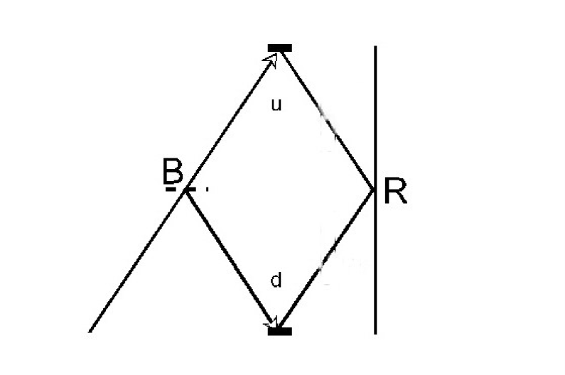
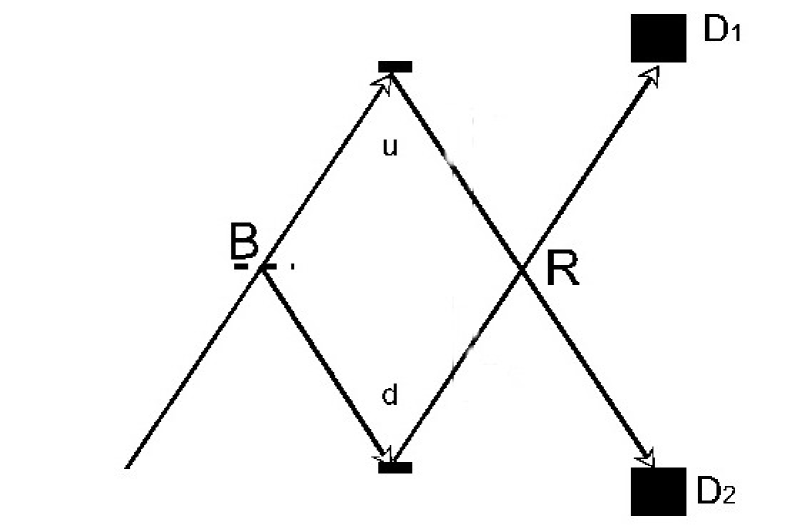
Figure 1: Delayed Choice Interferometer: interference (left); ”which path” (right)

The Bohm trajectories for pure states in this interferometer have been discussed extensively [ESSW92, DHS93, DFGZ93, ESSW93, AV96, Cun98, Scu98, CHM00, Mar02], in the context of the claim in [ESSW92] that the trajectories are ”surrealistic”.

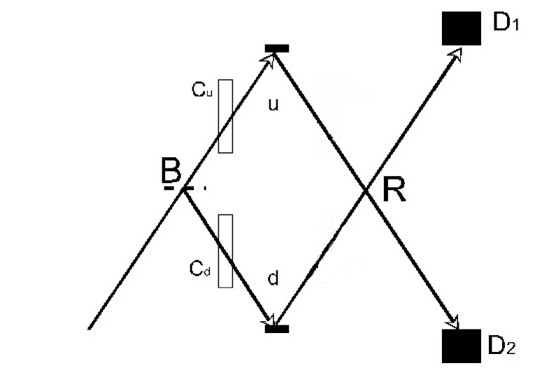
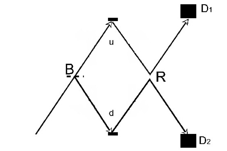
Figure 2: ”Which Path”: measured(left); not measured (right)

We will not revisit these arguments here but simply note that, when a measurement of the path is made while the particle is in the interferometer (by detectors $C_{u}$ and $C_{d}$) the Bohm trajectories follow the paths like Figure 2(left). In the absence of such a measurement, the Bohm trajectories for the particle are deflected in the interference region $R$ (Figure 2(right)) so ’fooling’ the delayed choice of ’which path’ made by detectors at $D_{1}$ and $D_{2}$.

For the density matrix we will be considering the same experimental arrangement, but the atomic state entering the arms of the interferometer (after the beam splitter region $B$) is the mixed state

$$\frac{1}{2}\left(\left|{{\phi_{u}(x,t_{1})}}\right\rangle\left.\left\langle{{\phi_{u}(x,t_{1})}}\right.\right|+\left|{{\phi_{d}(x,t_{1})}}\right\rangle\left.\left\langle{{\phi_{d}(x,t_{1})}}\right.\right|\right)$$ (56)

where $\phi_{u}$ represents a pure state in the upper arm of the interferometer and $\phi_{d}$ is a pure state in the lower arm. No interference effects are expected in the region $R$.

We will describe the Bohm trajectories for this in the cases where:

1. The mixed state is a physically real density matrix $\varrho$;

2. The mixed state is a statistical mixture $\rho$;

3. The mixed state is a physically real density matrix, and a measurement of the atomic location is performed while the atom is in the interferometer.

4.1 Physically real density matrix

While the atom is in the arms of the interferometer, the wavepacket corresponding to $\left|{{\phi_{u}}}\right\rangle$$\left.\left\langle{{\phi_{u}}}\right.\right|$ and that corresponding to $\left|{{\phi_{d}}}\right\rangle$$\left.\left\langle{{\phi_{d}}}\right.\right|$ are superorthogonal. The trajectories in the arms of the interferometer are much as we would expect. However, when the atomic trajectory enters the region $R$, both wavepackets start to overlap. The previously passive information in the wavepacket from the other arm of the interferometer becomes active again.

No interference fringes occur in the region $R$, and if phase shifters are placed in the arms of the interferometer, their settings have no effect upon the trajectories. However, the trajectories do change in $R$. The symmetry of the arrangement, and the ’no-crossing principle’ for the flow lines in a probability current, ensures that no actual trajectories can cross the center of the region $R$. The Bohm trajectories follow the ’surrealistic’ paths similar to those in Figure 2(right), even in the absence of phase coherence between the two arms of the interferometer.

4.2 Statistical Ensemble

We have seen that, even in the absence of phase coherence, the Bohm trajectories for the density matrix show the surrealistic behaviour. Does this represent an unacceptable flaw in the model? To answer this, we now consider the situation where the density matrix is a statistical ensemble of pure states. This situation should more properly be described, for the point of view of the Bohm approach, as a finite assembly of many individual systems.

First consider the assembly

$$\rho_{1} \equiv \left|{{\phi_{a_{1}}}}\right\rangle\left.\left\langle{{\phi_{a_{1}}}}\right.\right|\otimes\left|{{\phi_{a_{2}}}}\right\rangle\left.\left\langle{{\phi_{a_{2}}}}\right.\right|\otimes\left|{{\phi_{a_{3}}}}\right\rangle\left.\left\langle{{\phi_{a_{3}}}}\right.\right|\ldots$$ (57)

$$\equiv \Pi_{i}\left|{{\phi_{a_{i}}}}\right\rangle\left.\left\langle{{\phi_{a_{i}}}}\right.\right|$$

where $a_{i}=u$ or $d$ with a probability of one-half. As the assembly consists entirely of product states, the behaviour in each case is independant of the other cases.

If the state is $\left|{{\phi_{u}}}\right\rangle$$\left.\left\langle{{\phi_{u}}}\right.\right|$, then the trajectories pass down the u-branch, and go through the interference region without deflection. Similarly, systems in the $\left|{{\phi_{d}}}\right\rangle$$\left.\left\langle{{\phi_{d}}}\right.\right|$ state pass down the d-branch and are undeflected at $R$. These trajectories are what we would expect from an incoherent mixture.

However, now let us consider the assembly

$$\rho_{2}\equiv\Pi_{i}\left|{{\phi_{b_{i}}}}\right\rangle\left.\left\langle{{\phi_{b_{i}}}}\right.\right|$$ (58)

where $b_{i}=+$ or $-$ occur with equal probability and

$$\left|\phi_{+}\right\rangle = \frac{1}{\sqrt{2}}\left(\left|\phi_{u}\right\rangle+\left|\phi_{d}\right\rangle\right)$$ (59)

$$\left|\phi_{-}\right\rangle = \frac{1}{\sqrt{2}}\left(\left|\phi_{u}\right\rangle-\left|\phi_{d}\right\rangle\right).$$ (60)

This forms exactly the same statistical ensemble. Now, however, in each individual case there will be interference effects within the region $R$, it is just that the combination of these effects will cancel out over the ensemble. If we were to measure the state in the $(+,-)$ basis, then we would be able to correlate the measurements of this to the location of the atom on the screen and exhibit the interference fringes. The Bohm trajectories for the assembly $\rho_{2}$ all reflect in the region $R$ and display the supposed ’surrealistic’ behaviour.

There are no observable consequences of the choice of the different assemblies to construct the statistical ensemble. Consequently, if we are only given the density matrix of a statistical ensemble, we are unable to say which assembly it is constructed from and cannot simply assume that the underlying Bohm trajectories will follow the pattern in Figure 1. It is only legitimate to assume the trajectories will pass through the interference region undeflected if we know we have an assembly of $\left|\phi_{u}\right\rangle$ and $\left|\phi_{d}\right\rangle$ states, in which case the Bohm trajectories agree. Thus we conclude the behaviour of the trajectories for the physically real density matrix cannot be ruled out as unacceptable on these grounds.

4.3 Measuring the path

Finally, we consider what happens when we have the physically real density matrix

$$\varrho=\frac{1}{2}\left(\left|{{\phi_{u}(x,t_{1})}}\right\rangle\left.\left\langle{{\phi_{u}(x,t_{1})}}\right.\right|+\left|{{\phi_{d}(x,t_{1})}}\right\rangle\left.\left\langle{{\phi_{d}(x,t_{1})}}\right.\right|\right)$$ (61)

and we include a conventional measuring device in the u-path. The measuring device starts in the state $\left|\xi_{0}\right\rangle$. If the atom is in the state $\left|\phi_{u}\right\rangle$, the measuring device moves into the state $\left|\xi_{1}\right\rangle$. The states $\left|\xi_{0}\right\rangle$ and $\left|\xi_{1}\right\rangle$ are superorthogonal.

If we now apply the interaction to the initial state

$$\varrho\otimes\left|{{\xi_{0}}}\right\rangle\left.\left\langle{{\xi_{0}}}\right.\right|$$ (62)

the system becomes the correlated density matrix

$$\frac{1}{2}\left(\left|{{\phi_{u}\xi_{1}}}\right\rangle\left.\left\langle{{\phi_{u}\xi_{1}}}\right.\right|+\left|{{\phi_{d}\xi_{0}}}\right\rangle\left.\left\langle{{\phi_{d}\xi_{0}}}\right.\right|\right).$$ (63)

As we saw above, as the measuring device states are superorthogonal, the system behaves exactly as if it were the statistical ensemble. This is true even when the atomic states enter the region $R$. The Bohm trajectories of the atom pass undeflected through in the manner of Figure 2(left).

We conclude that the Bohm trajectories for the density matrix cannot be considered any more or less acceptable than the trajectories for the pure states.

5 CONCLUSION

By extending the de Broglie-Bohm interpretation to cover density matrices, we showed it was possible to consistently treat the density matrix as a property, not of an ensemble, but of an individual system.

It is worth asking why Bell seemed to suggest that this was not possible. An examination of [Bel80] shows that the density matrix Bell considered arose, not as a fundamental description of an individual system, but through tracing over part of an entangled system in an overall pure state, as in Equation 1.

Bell considers a pure state that interacts with a measuring device, in an arrangement similar to Figure 2(left). After the detectors have interacted with the atomic beam, the full state is:

$$\frac{1}{\sqrt{2}}\left(\left|\phi_{u}\xi_{1}\right\rangle+\left|\phi_{d}\xi_{0}\right\rangle\right).$$ (64)

Tracing over the detector states $\xi_{i}$ leaves the density matrix

$$\rho=\frac{1}{2}\left(\left|{{\phi_{u}}}\right\rangle\left.\left\langle{{\phi_{u}}}\right.\right|+\left|{{\phi_{d}}}\right\rangle\left.\left\langle{{\phi_{d}}}\right.\right|\right).$$ (65)

Bell wishes to construct trajectory solutions which resemble Figure 2(left) based on the density matrix for the atomic beam alone. This fails, as the entangled state trajectories are non-locally dependant upon the location of beable of the measuring device.

The symmetry of Equation 65 and the ’no-crossing’ principle ensure that a trajectory solution based upon the reduced density matrix alone must produce tracks as in Figure 2(right). It is only the superorthogonality of the detector states $\left|\xi_{i}\right\rangle$ that allows the atomic beam states to act as if they are a statistical ensemble of $\left|\phi_{i}\right\rangle$ states and cross over in the interference region.

However, the density matrix we have considered in this paper does not arise either as a reduced density matrix, or as a statistical ensemble of pure states. It is the complete description of an individual system. For this, we have shown that a consistent and coherent trajectory interpretation in the manner of the de Broglie-Bohm interpretation is possible.

References

- [AA98] Y Aharanov and J Anandan. ”Meaning of the density matrix”. 1998. quant-ph/9803018.
- [Alb00] D Z Albert. Time and Chance. 2000.
- [AV96] Y Aharanov and L Vaidman. ”About position measurements which do not show the Bohmian particle position”. In [CFG96], pages 141–154, 1996.
- [Bel80] J S Bell. ”de Broglie-Bohm, delayed-choice double-slit experiment, and density matrix”. International Journal of Quantum Chemistry, pages 155–159, 1980. in [Bel87].
- [Bel87] J S Bell. Speakable and unspeakable in quantum mechanics. Cambridge University Press, 1987.
- [BH93] D Bohm and B J Hiley. The Undivided Universe. Routledge, 1993.
- [BH96] D Bohm and B J Hiley. ”Statistical mechanics and the ontological interpretation”. Foundations of Physics, 26(6):823–846, 1996.
- [BH00] M Brown and B J Hiley. ”Schrödinger revisited: An algebraic approach”. 2000. quant-ph/0005026.
- [Boh52a] D Bohm. ”A suggested interpretation of the quantum theory in terms of ’hidden’ variables I”. Physical Review, 85:166–178, 1952.
- [Boh52b] D Bohm. ”A suggested interpretation of the quantum theory in terms of ’hidden’ variables II”. Physical Review, 85:179–193, 1952.
- [CFG96] J T Cushing, A Fine, and S Goldstein, editors. Bohmian Mechanics and Quantum Theory: An Appraisal. Kluwer, 1996.
- [CHM00] R E Callaghan, B J Hiley, and O J E Maroney. ”Quantum trajectories, real, surreal or an approximation to a deeper process?”. 2000. quant-ph/0010020.
- [CN01] I L Chuang and M A Nielsen. Quantum Computation and Quantum Information. Cambridge, 2001.
- [Cun98] M O T Cunha. ”What is surrealistic about Bohm trajectories?”. 1998. quant-ph/9809006.
- [DFGZ93] D Durr, W Fusseder, S Goldstein, and N Zanghi. ”Comment on surrealistic Bohm trajectories”. Z Naturforsch, 48a:1261–1262, 1993.
- [DHS93] C Dewdney, L Hardy, and E J Squires. ”How late measurements of quantum trajectories can fool a detector”. Phys Lett A, 184(1):6–11, 1993.
- [ESSW92] B G Englert, M O Scully, G Sussmann, and H Walther. ”Surrealistic Bohm trajectories”. Z Naturforsch, 47A:1175–1186, 1992.
- [ESSW93] B G Englert, M O Scully, G Sussmann, and H Walther. ”Reply to comment on surrealistic Bohm trajectories”. Z Naturforsch, 48a:1263–1264, 1993.
- [Hol93] P R Holland. The Quantum Theory of Motion. Cambridge, 1993.
- [HPMZ94] J J Halliwell, J Perez-Mercader, and W H Zurek, editors. Physical Origins of Time Asymmetry. Cambridge, 1994.
- [LR90] H S Leff and A F Rex, editors. Maxwell’s Demon. Entropy, Information, Computing. Adam Hilger, 1990.
- [Mar02] O J E Maroney. Information and Entropy in Quantum Theory. PhD thesis, Birkbeck College, University of London, 2002. www.bbk.ac.uk/tpru/OwenMaroney/thesis/thesis.html.
- [Per93] A Peres. Quantum Theory: Concepts and Methods. Kluwer, 1993.
- [Pop57] K R Popper. ”Irreversibility, or entropy since 1905”. Brit J Phil Sci, 8:151–155, 1957.
- [Scu98] M O Scully. ”Do Bohm trajectories always provide a trustworthy physical picture of particle motion?”. Physica Scripta, T76:41–46, 1998.
- [Uff01] J Uffink. ”Bluff your way in the second law of thermodynamics”. Studies in History and Philosophy of Modern Physics, 32(3):305–394, 2001.