An experimental demonstration of single photon nonlocality

Abstract

In this letter we experimentally implement a single photon Bell test based on the ideas of S. Tan et al. [Phys. Rev. Lett., 66, 252 (1991)] and L. Hardy [Phys. Rev. Lett., 73, 2279 (1994)]. A double heterodyne measurement is used to measure correlations in the Fock space spanned by zero and one photons. Local oscillators used in the correlation measurement are distributed to two observers by co-propagating it in an orthogonal polarization mode. This method eliminates the need for interferometrical stability in the setup, consequently making it a robust and scalable method.

For experimental Bell tests Bell (1964); Clauser et al. (1969) it has been a successful strategy to use polarization entangled photon pairs, either from atomic cascades Freedmann and Clauser (1972); Aspect et al. (1981, 1982a, 1982b), or parametric down-conversion Ou and Mandel (1988); Kwiat et al. (1995); Weihs et al. (1998); Kurtsiefer et al. (2001), or produced by post selecting a photon pair from independent sources Pittman and Franson (2003). In these experiments, it is observed that correlations between the two photons are incompatible with local realism, i.e. Bell’s inequalities are violated.

In 1991, Tan et al. proposed that it would be possible to show a contradiction between local realism and quantum mechanics using only a single particle Tan et al. (1991). The proposal spurred a debate, where the main argument against the feasibility of such an experiment was that detection of the particle at one location would prohibit the measurement of any property associated with that particle at another location. A counter argument was that this would indeed be true if one measured particle-like properties at the two locations, but if one instead chose to measure wave-like properties, the argument fails. Another criticism against Tan’s et al. proposal was that a measurement of wavelike properties requires a reference oscillator. Hence, measurements of wavelike properties of a single particle require additional particles. The notion of single particle non-locality was hence put in doubt Greenberger et al. (1995). Hardy, who had proposed an alternative experiment to demonstrate the non-locality of a single particle, then put forth operational criteria for such a test, where the main ingredient is that the demonstrated non-local properties should be dependent on the presence of a single particle Hardy (1994, 1995). If the quantum state is robbed of this particle, no non-local properties should be observed. That is, all the non-local correlations should be carried by a single-particle state, although the observation of these correlations may contain measurements on auxiliary reference particles. The state of these reference oscillators should be such that the observers can generate them using only classical communication and local operations.

In this letter we experimentally test the behavior of non-local correlations for one single photon using a setup similar to the one proposed by Tan et al. Tan et al. (1991). When a single photon passes a balanced beam splitter it has equal probability amplitudes for reflection and transmission. In the number basis such states have the form

$$\frac{1}{\sqrt{2}}\left[|1\rangle_{\mathrm{T}}|0\rangle_{\mathrm{R}}+|0\rangle_{\mathrm{T}}|1\rangle_{\mathrm{R}}\right],$$ (1)

where T (R) refers to the transmitted (reflected) channel of the beam splitter. This state is mathematically isomorphic to a two-photon Bell state encoded in horizontal (H) and vertical (V) polarization, with the replacements $|0\rangle\leftrightarrow|H\rangle$ and $|1\rangle\leftrightarrow|V\rangle$). Using (1) for a Bell experiment requires that measurements can be made in bases complementary to the number basis $|0\rangle$ and $|1\rangle$ in the two channels. This is not straightforward using photon counters, since quantities complementary to photon number are sought.

In Fig. 1 we illustrate two experimental implementations capable of performing measurements complementary to photon number measurement.

A signal from an experiment is mixed with a local oscillator (LO) on a beam splitter in such a way that a photon detector observing one photon is not capable of telling if the photon came from the experiment or the LO beam. If the photon came from the LO, there was zero photons coming from the experiment. If no photon came from the LO, there was one photon coming from the experiment. If the local oscillator is a coherent state $\left|\alpha\right\rangle$, amplitudes for these two events give projection on the wanted state:

$$\mathcal{N}\left(r\alpha\left|0\right\rangle+\left|1\right\rangle\right),$$ (2)

where $\mathcal{N}$ is a normalization constant, and $r\alpha$ is the complex amplitude for the LO in the counter mode. This is illustrated in Fig. 1(a) where $r\alpha$ is the amplitude for reflection of the local oscillator and in Fig. 1(b) where $r\alpha$ is the amplitude of the LO after the polarizer. The number states in Eq. (2) describe the photon number in the mode arriving from the experiment. For similar implementations where local oscillators are replaced by single photons we refer to the papers by F. Sciarrino et al. Sciarrino et al. (2002) and H. Lee et al. Lee and Kim (2000).

Figure 1: The photon counters are unable to tell if a detected photon came from the local oscillator (LO) or if it was a part of the signal from the experiment. If the two possible origins cannot be told apart, the amplitudes for the two possible events must be added. In a) the local oscillator is mixed with the signal on a beam splitter with high transmission. The polarization of the signal and LO are the same to ensure undistinguishable photons. In b) the polarization of the local oscillator is orthogonal to the signal beam, and the two beams co-propagates. By rotating a polarizer one can adjust the probability for transmitting the signal, or LO-photon. In both cases, interference filters are put before the detectors to erase path information stored in the energy spectrum of the photons.

In Fig. 2 we have a schematic description of the optical setup used for this experiment. The light source is a Ti:Sapphire laser which pumps a frequency doubler (1 mm LBO crystal), marked SHG in the figure, producing fs-pulses at 390 nm. These pulses pump a type-I down-converter (3 mm BBO crystal), yielding photon pairs at 780 nm emitted with a separation of 3 degrees from the pump beam. One of the photons (the idler) is sent through an interference filter and detected by an avalanche photodiode, $\mathrm{D}_{\mathrm{T}}$. Detection of the idler in $\mathrm{D}_{\mathrm{T}}$ indicates that the other photon of the pair (the signal) is present in the experiment. The polarization of the signal photon is made strictly vertical by a wave-plate and a polarizer. Afterwards, the signal photon propagates to one of the beam splitter input ports (BS).

To generate the local oscillator (LO) some light is picked off the main beam of the Ti:Sapphire laser. A delay line is adjusted so that the LO arrives at the beam splitter simultaneously with the single photon. Before the beam splitter the intensity is adjusted so that $r\alpha$ matches the single photon intensity to ensure high visibility in the correlation measurement (See discussion following Eq. 9).

The polarization of the LO is adjusted to be strictly orthogonal to the signal photon polarization with another wave-plate and polarizer. After the beam splitter each arm is equipped with a polarizer oriented so that it transmits a LO photon or a single photon with equal probability. Because the LO has much higher intensity than the single photon beam the polarizer is set around 2 degrees. The single photon and the local oscillator co-propagates after the beam splitter. This eliminates the need to stabilize the relative phase of the local oscillators in the two arms Björk et al. (2002). This is the main difference between our implementation and the setup proposed in Tan et al. (1991). The relative phase between the two local oscillators is adjusted by tilting a thin quartz plate around its optics axis in one arm. The optic axis of the quartz plate is parallel to the single photon polarization.

After the polarizers the light is coupled into single mode optical fibers preceded by interference filters (FWHM 3nm) and followed by silicon avalanche photodiodes. The signals from the APDs are correlated and recorded by a computer.

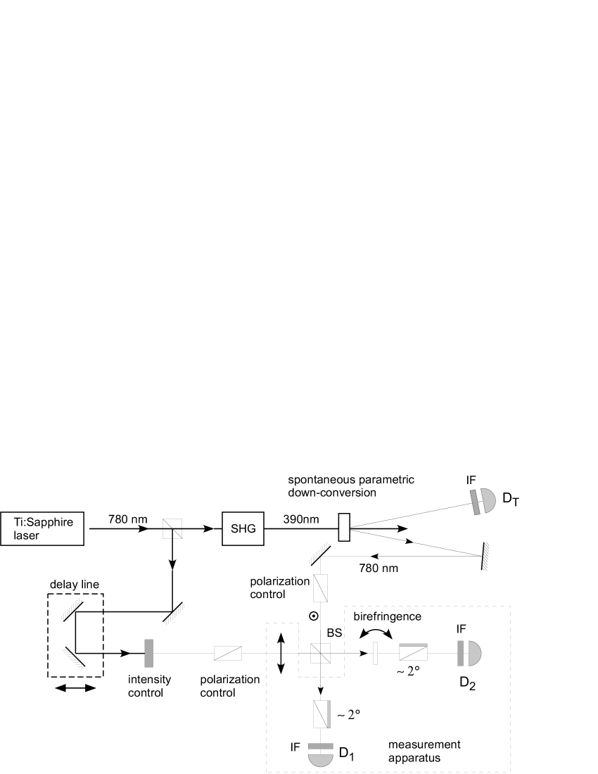
Figure 2: Experimental setup: A single photon produced in spontaneous parametric down-converter is overlapped with a coherent local oscillator on a 50/50 beam splitter. In each output mode of the beam splitter we place the detectors described in Fig. 1. To change the relative phase of the local oscillators we tilt a birefringent quartz plate in one of the arms.

In the optical setup illustrated in Fig. 2 the single photon enters the beam splitter (BS) from above and the LO photon from the left. This state is $\left|1,0\right\rangle_{\mathrm{signal}}\otimes\left|0,\sqrt{2}\alpha\right\rangle_{\mathrm{LO}}$, where the two modes at each location refer to the different polarizations of the single photon channel and the local oscillator, respectively. After the beam splitter the state is (ignoring phase factors obtained upon reflection):

$$\left|\Psi\right\rangle=\frac{1}{\sqrt{2}}(\left|1,\alpha\right\rangle_{\mathrm{T}}\left|0,\alpha^{\prime}\right\rangle_{\mathrm{R}}+\left|0,\alpha\right\rangle_{\mathrm{T}}\left|1,\alpha^{\prime}\right\rangle_{\mathrm{R}}),$$ (3)

where the subscripts $T$ and $R$ refer to the transmitted and reflected output arms, respectively. The coherent states are described by $\alpha=|\alpha|e^{i\theta}$ and $\alpha^{\prime}=|\alpha|e^{i\theta^{\prime}}$. The two modes in each arm refer to polarization. We define creation operators for these modes as:

$$\hat{a}^{{\dagger}}_{\mathrm{k}}\left|0,0\right\rangle_{\mathrm{k}} = \left|1,0\right\rangle_{\mathrm{k}},$$

$$\hat{b}^{{\dagger}}_{\mathrm{k}}\left|0,0\right\rangle_{\mathrm{k}} = \left|0,1\right\rangle_{\mathrm{k}},$$

where the subscript $\mathrm{k}$ refers to the two channels R and T. The state (3) is analyzed using a polarizer described by the transmittance $t$ and the reflectance $r$. The unitary transformation for this device relates the transmitted (reflected) mode $c$ ($d$) to the incoming modes $a$ and $b$ in the following way:

$$\begin{array}[]{cc}\left\{\begin{array}[]{l}c_{\mathrm{k}}^{\dagger}=ta_{\mathrm{k}}^{\dagger}+rb_{\mathrm{k}}^{\dagger}\\ d_{\mathrm{k}}^{\dagger}=-ra_{\mathrm{k}}^{\dagger}+tb_{\mathrm{k}}^{\dagger}\end{array}\right.&\Leftrightarrow\left\{\begin{array}[]{l}a_{\mathrm{k}}^{\dagger}=tc_{\mathrm{k}}^{\dagger}-rd_{\mathrm{k}}^{\dagger}\\ b_{\mathrm{k}}^{\dagger}=rc_{\mathrm{k}}^{\dagger}+td_{\mathrm{k}}^{\dagger}\end{array}\right.\end{array}$$

Later, we will be interested in the transmitted channels $c_{\mathrm{k}}$, where our detectors are placed. Rewriting the state (3) using the above creation operators we have:

$$\left|\Psi\right\rangle = \frac{1}{\sqrt{2}}(\left|1,\alpha\right\rangle_{\mathrm{T}}\left|0,\alpha^{\prime}\right\rangle_{\mathrm{R}}+\left|0,\alpha\right\rangle_{\mathrm{T}}\left|1,\alpha^{\prime}\right\rangle_{2})$$

$$= D_{b_{\mathrm{T}}}(\alpha)D_{b_{\mathrm{R}}}(\alpha^{\prime})\frac{1}{\sqrt{2}}(\hat{a}^{{\dagger}}_{\mathrm{T}}+\hat{a}^{{\dagger}}_{\mathrm{R}})\left|0,0\right\rangle_{\mathrm{T}}\left|0,0\right\rangle_{\mathrm{R}}$$

$$\rightarrow D_{c_{\mathrm{T}}}(r\alpha)D_{d_{\mathrm{T}}}(t\alpha)D_{c_{\mathrm{R}}}(r\alpha^{\prime})D_{d_{\mathrm{R}}}(t\alpha^{\prime})\times$$

$$(t\hat{c}^{{\dagger}}_{\mathrm{T}}-r\hat{d}^{{\dagger}}_{\mathrm{T}}+t\hat{c}^{{\dagger}}_{\mathrm{R}}-r\hat{d}^{{\dagger}}_{\mathrm{T}})\left|0,0\right\rangle_{\mathrm{T}}\left|0,0\right\rangle_{\mathrm{R}}$$

$$= (t\hat{c}^{{\dagger}}_{\mathrm{T}}-r\hat{d}^{{\dagger}}_{\mathrm{T}}+t\hat{c}^{{\dagger}}_{\mathrm{R}}-r\hat{d}^{{\dagger}}_{\mathrm{R}})\left|r\alpha,t\alpha\right\rangle_{\mathrm{T}}\left|r\alpha^{\prime},t\alpha^{\prime}\right\rangle_{\mathrm{R}},$$

where $\left|0,0\right\rangle_{\mathrm{T}}\left|0,0\right\rangle_{\mathrm{R}}$ is the vacuum state of the four modes. The probability for the two detectors to click simultaneously is given by:

$$\mathrm{P_{coincidence}}=1-(D_{1}+D_{2}-D_{12})$$ (7)

where $D_{1}$ ($D_{2}$) is the probability that detector $1$ ($2$) registers nothing irrespective of what happens in the other detectors. The term $D_{12}$ balances for the double count of the event ”nothing in both detectors”. We use this measure instead of photon number correlation because our detectors only register the presence of photons and are unable to resolve the photon number.

To calculate these different probabilities we use the following projection operators:

$$\hat{\mathrm{P}}_{1} = |0\rangle\langle 0|\otimes\mathbf{1}\otimes\mathbf{1}\otimes\mathbf{1}$$

$$\hat{\mathrm{P}}_{2} = \mathbf{1}\otimes\mathbf{1}\otimes|0\rangle\langle 0|\otimes\mathbf{1}$$

$$\hat{\mathrm{P}}_{12} = |0\rangle\langle 0|\otimes\mathbf{1}\otimes|0\rangle\langle 0|\otimes\mathbf{1},$$

where the spaces refer, in order to the modes $c_{\mathrm{T}}$, $d_{\mathrm{T}}$, $c_{\mathrm{R}}$, and $d_{\mathrm{R}}$. Using the above definitions of $\hat{\mathrm{P}}_{i}$ and $\left|\Psi\right\rangle$ one finds:

$$D_{1} = \left\langle\Psi\right|\hat{\mathrm{P}}_{1}\left|\Psi\right\rangle=\frac{1}{2}e^{-|r\alpha|^{2}}(1+r^{2}+r^{2}t^{2}|\alpha|^{2}).$$

$$D_{2} = \left\langle\Psi\right|\hat{\mathrm{P}}_{2}\left|\Psi\right\rangle=\frac{1}{2}e^{-|r\alpha|^{2}}(1+r^{2}+r^{2}t^{2}|\alpha|^{2}).$$

$$D_{12} = \left\langle\Psi\right|\hat{\mathrm{P}}_{12}\left|\Psi\right\rangle=e^{-2|r\alpha|^{2}}(r^{2}+2r^{2}t^{2}|\alpha|^{2}\cos^{2}\frac{\theta-\theta^{\prime}}{2}).$$

This yields the coincidence probability:

$$\mathrm{P_{coincidence}}=1-e^{-|r\alpha|^{2}}(1+r^{2}+r^{2}t^{2}|\alpha|^{2})$$

$$+e^{-2|r\alpha|^{2}}(r^{2}+2r^{2}t^{2}|\alpha|^{2}\cos^{2}\frac{\theta-\theta^{\prime}}{2}).$$ (8)

In addition to these coincidences, we also have the case with zero photons arriving in the single photon channel. Coincidences are registered also in this case when two photons from the LO are detected. The probability for these false coincidence counts is easily calculated in the same way as above:

$$\mathrm{P_{coincidence}^{\mathrm{false}}} = (1-e^{-|r\alpha|^{2}})^{2}$$ (9)

This may also be verified easily through a different reasoning: The probability of having more than zero LO photons in one arm is given by $1-e^{-|r\alpha|^{2}}$. The probability of having photons in both arms is this probability squared.

The total probability for the two detectors to register photons simultaneously is given by

$$\mathrm{P_{coincidence}^{\mathrm{tot}}}=\eta\mathrm{P_{coincidence}}+(1-\eta)\mathrm{P_{coincidence}^{\mathrm{false}}}$$

where $\eta$ is the quantum efficiency of the triggered photon source (For the setup: $\eta\sim 10^{-2}$). To minimize the influence of the false coincidences we choose $r\ll t$ and $|r\alpha|$ small to minimize the influence of $\mathrm{P_{coincidence}^{\mathrm{false}}}$. This choice introduces a trade-off between the implementation of the projectors described by Eq. (2) and the goal to minimize the influence of false coincidences. Practically, the lower bound of $|r\alpha|$ is determined by the detection rate allowed by the laser stability.

In Fig. 3 we plot the measured correlation obtained in the setup illustrated in Fig. 2. The birefringent plate is rotated around the optic axis so that relative phase shifts between -70 and 350 degrees are introduced in the two arms. If either the single photon or the local oscillator is missing, we measure a flat, phase independent correlation curve. Similarly, the signal intensity in each detector is almost constant as the phase shift is varied. Introducing a quarter-wave plate, with the optical axis horizontal or vertical, in either arm shifts the fringe pattern 90 degrees with negligible loss in visibility.

This experiment is limited by multiple down-conversion events since we chose to work at high UV-intensities (350 mW) to reduce measurement times. With the local oscillator blocked, we detect about one triple coincidence per second due to multiple down-conversion pair production. Reduced intensity increases visibility, see Pittman and Franson Pittman and Franson (2003) for details on this topic.

In our experiment we have raw correlation data with a visibility $66\pm 2\%$. This curve consists of three contributions: i) The two photons arriving to detectors $D_{1}$ and $D_{2}$ originate from LO and single photon source (phase shift dependent). ii) The two photons both come from the LO (constant under phase shift:  2.5 $s^{-1}$). iii) The two photons both come from the single photon source (constant under phase shift:  1.0 $s^{-1}$). If the coincidences corresponding to these two backgrounds are subtracted from the signal, the visibility becomes $91\pm 3\%$.

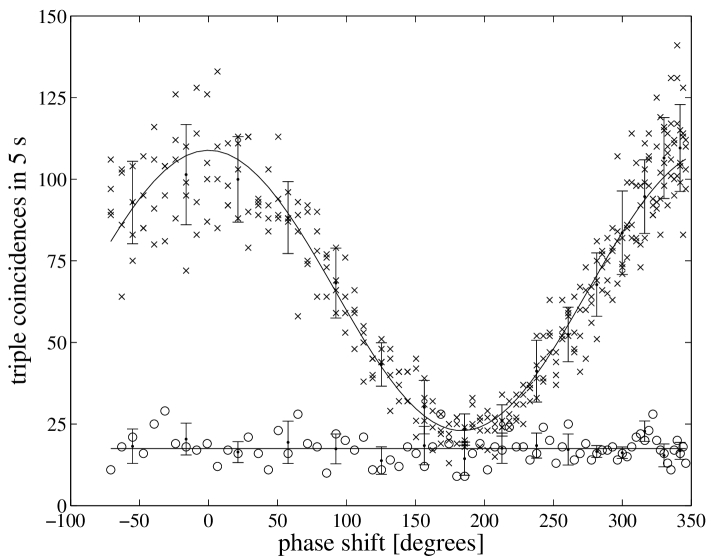
Figure 3: Experimental data and curve fits. The oscillating curve shows the correlation between the two detectors as the phase shift is varied. The flat curve shows the correlation background due to multiple photons from the single photon source and the local oscillator. The visibility for the correlation curve is $91\pm 3\%$ and $66\pm 2\%$ with and without corrections for background correlations. These visibilities should be compared with the 71% limit for violation of Bells inequalities.

It should be noted that it is possible to use different photon states as the input state to the beam splitter (BS in Fig. 2). If the state remains separable after the beam splitter, only classical correlations are expected. We performed such tests using phase modulated coherent light instead of single photons. Theoretically we would expect the correlation to reach the maximally allowed 50 % limit for this classical correlation. Experimentally we create this coherent field by splitting off light from the local oscillator to the polarization control of the single photon channel (See Fig. 2). The phase modulation is provided by another delay line modifying the propagation distance. Using this setup we measured a correlation visibility of $48\pm 2\%$, just below the classical limit. This visibility indicates a well aligned system and that we don’t observe Bell-type correlations in the local oscillator.

The representation of quantum information as a superposition particle number states, $\alpha\left|0\right\rangle+\beta\left|1\right\rangle$ instead of superimposing different modes offers certain advantages. Using this representation makes it is feasible to perform quantum computations with linear operations and feedback from measurements Knill et al. (2001). To perform interesting experiments on these qubits, it is desirable to have access to precise quantum mechanical observables in this space and specifically those with eigenstates that are superpositions of number states ($\left|0\right\rangle+e^{i\theta}\left|1\right\rangle$). Here we have presented a robust non-interferometric method for the implementation of such observables. This experimental scheme may be scaled up to include perform correlation measurements on multiphoton states. Using the criteria for single particle non-locality set up by Hardy Hardy (1995), we have performed an experiment that supports the prediction of Tan et al. of single particle non-locality Tan et al. (1991).

We gratefully acknowledge useful discussions with Drs. Marie Ericsson, Per Jonsson and Phil Marsden. This work was financially supported by Swedish Research Council (VR), STINT and INTAS.

References

- Bell (1964) J. S. Bell, Physics 1, 195 (1964).
- Clauser et al. (1969) J. F. Clauser, M. A. Horne, A. Shimony, and R. A. Holt, Phys. Rev. Lett. 23, 880 (1969).
- Freedmann and Clauser (1972) S. J. Freedmann and J. F. Clauser, Phys. Rev. Lett. 28, 938 (1972).
- Aspect et al. (1981) A. Aspect, P. Grangier, and G. Roger, Phys. Rev. Lett. 47, 460 (1981).
- Aspect et al. (1982a) A. Aspect, P. Grangier, and G. Roger, Phys. Rev. Lett. 49, 91 (1982a).
- Aspect et al. (1982b) A. Aspect, J. Dalibard, and G. Roger, Phys. Rev. Lett. 49, 1804 (1982b).
- Ou and Mandel (1988) Z. Y. Ou and L. Mandel, Phys. Rev. Lett. 61, 50 (1988).
- Kwiat et al. (1995) P. G. Kwiat, K. Mattle, H. Weinfurter, A. Zeilinger, A. V. Sergienko, and Y.Shih, Phys. Rev. Lett. 75, 4337 (1995).
- Weihs et al. (1998) G. Weihs, T. Jennewein, C. Simon, H. Weinfurter, and A. Zeilinger, Phys. Rev. Lett. 81, 5039 (1998).
- Kurtsiefer et al. (2001) C. Kurtsiefer, M. Oberparleiter, and H. Weinfurter, Phys. Rev. A 64, 023802 (2001).
- Pittman and Franson (2003) T. B. Pittman and J. D. Franson, Phys. Rev. Lett. 90, 240401 (2003).
- Tan et al. (1991) S. M. Tan, D. F. Walls, and M. J. Collett, Phys. Rev. Lett. 66, 252 (1991).
- Greenberger et al. (1995) D. Greenberger, M. Horne, and A. Zeilinger, Phys. Rev. Lett. 75, 2064 (1995).
- Hardy (1994) L. Hardy, Phys. Rev. Lett. 73, 2279 (1994).
- Hardy (1995) L. Hardy, Phys. Rev. Lett. 75, 2065 (1995).
- Sciarrino et al. (2002) F. Sciarrino, E. Lombardi, G. Milani, and F. De Martini, Phys. Rev. A66, 024309 (2002).
- Lee and Kim (2000) H.-W. Lee and J. Kim, Phys. Rev. A63, 012305 (2000).
- Björk et al. (2002) G. Björk, P. Jonsson, and L. L. Sánches-Soto, Phys. Rev. A64, 042106 (2002).
- Knill et al. (2001) E. Knill, R. Laflamme, and G. J. Milburn, Nature 409, 46 (2001).