Noise enhancing the classical information capacity of a quantum channel

Abstract

We present a simple model of quantum communication where a noisy quantum channel may benefit from the addition of further noise at the decoding stage. We demonstrate enhancement of the classical information capacity of an amplitude damping channel, with a predetermined detection threshold, by the addition of noise in the decoding measurement.

I Introduction

In common wisdom, randomness and noise are thought to be detrimental to any physical process, especially at a quantum level, and hence also for the ability of the system to encode and process quantum information Nie00 . For classical systems the advent of phenomena such as stochastic resonance, Brownian ratchets, and Parrondo effects, have shown that noise may indeed play a helpful role after all Gam98 ; Par00 . This opens up the intriguing question of whether randomness can play a useful role in quantum systems Man02 , particularly due to the widespread current interest in quantum information schemes Lee02 .

In this paper we consider the quantum communication scenario, and present a toy model where the noise plays a positive role. In particular, given a noisy quantum channel, we shall show that the addition of noise at the decoding stage can improve the channel capacity.

II The model

Let us consider a simple communication model as depicted in Fig.1. At the sending station, classical information is encoded into quantum states, which in turn are sent through a noisy quantum channel. At the receiving station a decoding procedure is performed with the addition of noise to the decoding operation.

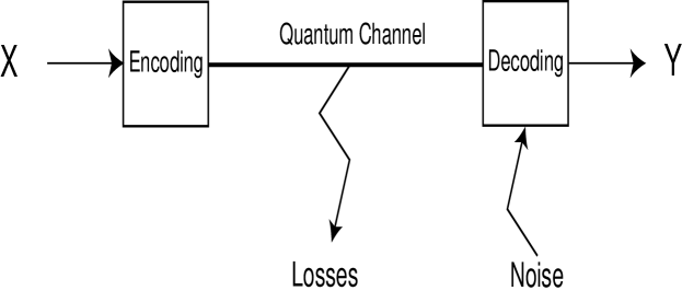
Figure 1: Schematic representation of the channel under study.

In detail, we consider an input random binary variable $X$ taking values $0$, $1$ and we encode it into quantum states according to the following rule,

$$\left\{\begin{array}[]{l}0\longrightarrow{\hat{\rho}}_{0}=|0\rangle\langle 0|\\ 1\longrightarrow{\hat{\rho}}_{1}=e^{-r^{2}}\sum_{n}\frac{r^{2n}}{n!}|n\rangle\langle n|\end{array}\right.\,,$$ (1)

where ${\hat{\rho}}_{1}$ is a completely dephased coherent state of amplitude $r\neq 0$. We then take the noisy quantum channel to be an amplitude damping channel ${\hat{\cal E}}$ Nie00 , the effect of which can be described by the map $r\to re^{-\tau}$, with $\tau$ a parameter determining the amount of amplitude damping. Finally, the output variable $Y$ is determined by a decoding procedure involving a quadrature measurement, through the Probability Operator Measure (POM) $d{\hat{\Pi}}(y)=\delta\left(y-{\hat{y}}\right)dy$ Hel76 ; Dar97 . The binary character of $Y$ comes out from a threshold detection of the type,

$$\left\{\begin{array}[]{l}|y|<\theta\longrightarrow 0\\ |y|>\theta\longrightarrow 1\end{array}\right.\,,$$ (2)

where $\theta$ represents a fixed threshold.

At this point, additional noise may be introduced at the decoding stage, such that we obtain a broadening of the POM Dar97 , that is,

$$d{\hat{\Pi}}(y)=\frac{1}{\sqrt{\pi\sigma^{2}}}\exp\left[-\frac{\left(y-{\hat{y}}\right)^{2}}{\sigma^{2}}\right]dy\,,$$ (3)

where $\sigma$ is the width of the Gaussian noise. For $\sigma\to 0$ the measurement converges to the ideal POM. The above kind of noise may be used to describe detection with non-unit efficiency Dar97 .

The output conditional probability between $Y$ and the input amplitude $r$ can be formally written as,

$$p(y|r) = {\rm Tr}\left\{{\hat{\cal E}}({\hat{\rho}})\int d{\hat{\Pi}}\right\}$$

$$= \int dy^{\prime}\langle y^{\prime}|{\hat{\cal E}}({\hat{\rho}})|y^{\prime}\rangle\frac{1}{\sqrt{\pi\sigma^{2}}}\exp\left[-\frac{\left(y-y^{\prime}\right)^{2}}{\sigma^{2}}\right]\,,$$

with,

$$\langle y^{\prime}|{\hat{\cal E}}({\hat{\rho}})|y^{\prime}\rangle=\left(\frac{1}{\pi}\right)^{1/2}\exp\left[-(y^{\prime})^{2}-r^{2}e^{-2\tau}\right]\sum_{n}\frac{\left(r^{2}e^{-2\tau}/2\right)^{n}}{(n!)^{2}}H_{n}^{2}(y^{\prime})\,,$$ (5)

where $H_{n}(.)$ denotes the Hermite polynomial of degree $n$. Explicitly, one has,

$$p(y|r) = \frac{1}{\sqrt{\pi(1+\sigma^{2})}}\exp\left[-r^{2}e^{-2\tau}-\frac{y^{2}}{1+\sigma^{2}}\right]$$ (6)

$$\times\sum_{n=0}^{\infty}\sum_{k=0}^{n}\frac{\left(r^{2}e^{-2\tau}/2\right)^{n}}{\left[(n-k)!\right]^{2}}\frac{2^{k}}{k!}\left(\frac{1}{1+\sigma^{2}}\right)^{n-k}H_{2n-2k}\left(\frac{y}{\sqrt{1+\sigma^{2}}}\right)\,.$$

By virtue of Eqs.(1) and (2), we obtain the binary transition probabilities for the input-output states,

$$p_{00} = \int_{I}p(y|0)dy\,,$$ (7)

$$p_{01} = \int_{I}p(y|r)dy\,,$$ (8)

$$p_{10} = \int_{{\bf R}-I}p(y|0)dy=1-p_{00}\,,$$ (9)

$$p_{11} = \int_{{\bf R}-I}p(y|r)dy=1-p_{01}\,,$$ (10)

where $I\equiv(-\theta,\theta)$. Expanding the expressions for the transition probabilities leads to,

$$p_{00} = {\rm Erf}\left(\frac{\theta}{\sqrt{1+\sigma^{2}}}\right)\,,$$ (11)

$$p_{01} = \frac{2}{\sqrt{\pi}}\exp\left[-r^{2}e^{-2\tau}\right]\sum_{n=0}^{\infty}\sum_{k=0}^{n}\frac{\left(r^{2}e^{-2\tau}/2\right)^{n}}{\left[(n-k)!\right]^{2}}\frac{2^{k}}{k!}\left(\frac{1}{1+\sigma^{2}}\right)^{n-k}$$ (12)

$$\times\left[H_{2n-2k-1}(0)-e^{-\theta^{2}/(1+\sigma^{2})}H_{2n-2k-1}\left(\frac{\theta}{\sqrt{1+\sigma^{2}}}\right)\right]\,.$$

with the other two transistion probabilities determined according to Eqs.(9) and (10). The maximum rates of information transfer may then be determined by maximizing over the input distribution.

III Channel capacity

Let $p_{0}$ and $p_{1}=1-p_{0}$ the input probabilities for the values $0$ and $1$, respectively. The output entropy of the channel is given by the Shannon entropy of the variable $Y$ Nie00 , that is

$$H(Y)={\cal H}\Big{(}p_{11}p_{1}+(1-p_{00})(1-p_{1})\Big{)}+{\cal H}\Big{(}(1-p_{11})p_{1}+p_{00}(1-p_{1})\Big{)}\,,$$ (13)

with the function ${\cal H}(z)=-z\log(z)$. Furthermore, the conditional entropy for $Y$ given $X$ is determined by Nie00 ,

$$H(Y|X)=(1-p_{1}){\cal H}(p_{00})+(1-p_{1}){\cal H}(1-p_{00})+p_{1}{\cal H}(p_{11})+p_{1}{\cal H}(1-p_{11})\,.$$ (14)

The channel capacity may then be obtained by maximizing the mutual information $H(Y)-H(Y|X)$, over all possible input probabilities Nie00 , explicitly,

$$C=\max_{\{p_{1}\}}\left[H(Y)-H(Y|X)\right]\,.$$ (15)

The input probability maximizing Eq.(15) may be shown to be,

$$p_{1}^{*}=\frac{p_{00}-\wp}{p_{00}+p_{11}-1}\,,$$ (16)

with,

$$\wp^{-1}=1+\exp\left[\ln(2)\;\frac{{\cal H}(p_{00})+{\cal H}(1-p_{00})-{\cal H}(p_{11})-{\cal H}(1-p_{11})}{p_{00}+p_{11}-1}\right]\,.$$ (17)

In Fig.2 we graph the capacity $C$ versus the noise strength $\sigma$ for different values of the threshold $\theta$, when the encoding amplitude and channel damping are fixed to $r=5$ and $\tau=0.5$ respectively. One can see that when the threshold $\theta$ becomes higher than the damped amplitude $re^{-\tau}$, the addition of the noise improves the distinguishability between the two outputs in the decoding stage, thus increasing the capacity. Clearly, there is an optimal strength value for the noise to be added, beyond which the capacity goes to zero.

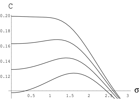
Figure 2: Channel capacity as function of the noise strength $\sigma$. Curves from top to bottom are for threshold values $\theta=3.6$, $3.8$, $4.0$ and $4.2$. The value of amplitude and damping parameters are $r=5$ and $\tau=0.5$.

IV Conclusion

In conclusion, we have shown the noise enhancement of the classical information capacity of a quantum communication channel. Analogous results have previously been found within the classical context Cha97 . The effect can be ascribed to the ability of the noise to induce transitions on the threshold Gam98 , and in our case it results from competition between two differing types of noise Man01 , the noise causing losses in the channel, and the noise broadening the POM.

The noise benefit could be optimized by a suitable tailoring of the POM and of the involved parameters, but this requires large numerical resources. Nonetheless, the present simple model can serve as a proof of principle and as a useful tool for further developments in more realistic schemes. In particular it could be relevant for systems that are constrained to receive signals through a fixed threshold Hel76 .

Our approach paves the way for a thorough study of noise effects in nonlinear quantum channels. Furthermore, the addition of stochastic noise on a channel may be helpful for quantum binary decision, which find applications in a variety of quantum measurement problems Hel76 .

On the other hand, quantum correlations (entanglement) have been exploited to improve both channel capacity Mac02 and quantum binary decision Dar02 . It would be interesting to compare the two approaches and to eventually combine them.

References

- (1) M. A. Nielsen and I. L. Chuang, Quantum computation and Quantum Information, (Cambridge University Press, Cambridge, 2000).
- (2) L. Gammaitoni, P. Hanggi, P. Jung and F. Marchesoni, Rev. Mod. Phys. 70, 223 (1998).
- (3) J. M. R. Parrondo, G. P. Harmer and D. Abbott, Phys. Rev. Lett. 85, 5226 (2000); G. P. Harmer, D. Abbott, P. G. Taylor and J. M. R. Parrondo, Chaos 11, 705 (2001).
- (4) S. Mancini, D. Vitali, P. Tombesi and R. Bonifacio, Europhys. Lett. 60, 498 (2002).
- (5) C. F. Lee and N. F. Johnson, Phys. Lett. A 301, 343 (2002).
- (6) C. W. Helstrom, Quantum Detection and Estimation Theory, (Academic Press, New York, 1976).
- (7) G. M. D’Ariano, Quantum Estimation Theory and Optical Detection, in Quantum Optics and Spectroscopy of Solids, T. Hakioglu and S. Shumovsky Eds. (Kluwer, Amsterdam, 1997), p.139.
- (8) F. Chapeau-Blondeau, Phys. Rev. E 55, 2016 (1997).
- (9) S. Mancini and R. Bonifacio, Phys. Rev. A 64, 032308 (2001).
- (10) C. Macchiavello and M. G. Palma, Phys. Rev. A 65, 050301 (2002).
- (11) G. M. D’Ariano, M. G. A. Paris and P. Perinotti, Phys. Rev. A 65, 062106 (2002).