Non-linear and quantum optics of a type II OPO containing a birefringent element Part 2 : bright entangled beams generation

Abstract

We describe theoretically the quantum properties of a type-II Optical Parametric Oscillator containing a birefringent plate which induces a linear coupling between the orthogonally polarized signal and idler beams and results in phase locking between these two beams. As in a standard OPO, the signal and idler waves show large quantum correlations which can be measured experimentally due to the phase locking between the two beams. We study the influence of the waveplate on the various criteria characterizing quantum correlations. We show in particular that the quantum correlations can be maximized by using optimized quadratures.

1 Introduction

The domain of quantum information with intense light beams is becoming more and more studied as practical applications are developed teleportkimble ; grangier ; leuchs . A large number of experiments rely on so-called EPR beams, that is a pair of fields containing quantum correlations on two different non commuting observables epr . Several methods have been used to date. One way to generate them is to mix two independent squeezed beams produced by two independent OPOs below threshold teleportkimble ; eprbachor , or to use third order non linearity in a fiber leuchs . Another configuration consists in using a non degenerate OPO below threshold eprkimble ; eprtaiyuan ; eprpolzik . We propose here a new method where two bright entangled beams are produced directly at the output of a non degenerate OPO pumped above threshold.

Optical Parametric Oscillators are very efficient sources of non classical light taiyuan ; kimblevidesq ; mertz ; mlynek ; zhang ; mescond . In particular, it has been shown experimentally that the intensities of the signal and idler beams exhibit very large quantum correlations taiyuan ; mertz ; mescond . It is also predicted that the phase of the signal and idler should show quantum anticorrelations reynaud . However, the measurement of these phase anticorrelations is not possible in a standard OPO in which frequency degenerate operation occurs only accidentally and is very sensitive to thermal and mechanical drifts. Thus, in practical experiments, the frequencies of the signal and idler beam are different. This implies that the relative phase between the two fields has a rapidly varying component. Furthermore, even if the device is actively stabilized on the frequency degeneracy working point pfister , this relative phase between signal and idler undergoes a diffusion process courtois , similarly to the phase of a laser field. In order to be able to measure experimentally these phase anticorrelations, one can use a phase locked OPO : one possible technique proposed in wong is to use a birefringent plate inserted inside the OPO cavity and making an angle with the axis of the non-linear crystal which leads to self-phase locking. This phenomenon has been studied in detail in fabre ; part1 at the classical level. It is the purpose of this paper to evaluate the influence of the phase locking mechanism on the quantum properties of the system.

The paper is organized as follows. In section 2, we give the equations describing the quantum fluctuations of the system. We study in section 3 the noise spectra of the amplitude quadratures difference and phase quadratures sum showing quantum noise reduction, i.e that these variances are below what would be observed for independent coherent states. In section 4, various entanglement criteria are discussed, namely EPR correlation properties (section 4.1), inseparability criterion (section 4.2) and teleportation fidelity (section 4.3). Finally, section 5 is devoted to the case of non-orthogonal quadratures which enable us to increase dramatically the violation of the inseparability criterion.

2 Basic equations

In order to calculate the fluctuations for the signal and idler fields when the OPO is pumped above threshold, we apply the input-output linearization technique described e.g. in fabre90 . We first determine the classical stationary solutions of the evolution equations : these solutions are denoted $A_{i}^{(s)}$ where $i=0,1,2$ corresponds to the pump, signal and idler fields. We then linearize the evolution equations around these stationary values by setting : $A_{i}=A_{i}^{(s)}+\delta A_{i},\,i=0,\,1,\,2$. Introducing the input fluctuations in all the modes, we obtain a set of linear coupled equations for the fluctuations of the different fields. By solving these equations in the Fourier domain, one can calculate the individual noise spectra as well as the correlations between the different quadratures.

Let us recall the system under study which has been discussed in detail in part1 . We consider a $\chi^{(2)}$ medium placed inside a ring optical cavity doubly resonant for signal and idler (fig. 1).

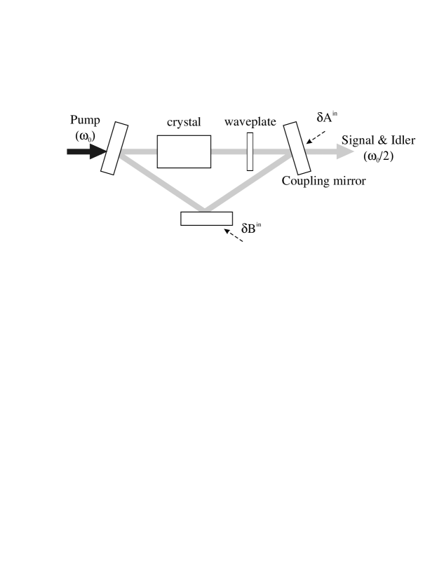
Figure 1: Ring cavity OPO with the fluctuations corresponding to the fluctuations coming through the input mirror ($\delta A_{i}^{in}$) and the fluctuations due to the losses ($\delta B_{i}^{in}$).

Type-II phase-matching results in orthogonally polarized signal and idler fields. The reflection coefficients for signal and idler are assumed to be equal in module : $r_{j}=r\exp(i\zeta_{j}),\,j=1,2$. We assume also that the cavity has a high finesse for these modes so that we can write $r=1-\kappa$ with $\kappa\ll 1$ ; the transmission is thus $t\approx\sqrt{2\kappa}$. Finally, the cavity is characterized by the round-trip losses for the signal and idler waves (crystal absorption, surface scattering), $\mu$, and we define a generalized reflection coefficient : $r^{\prime}=r(1-\mu)\approx 1-(\mu+\kappa)=1-\mu^{\prime}$.

Let us denote $l$ the crystal length and $L$ the free propagation length inside the cavity. The crystal indices of refraction are $n_{1}$ and $n_{2}$ respectively for the signal and idler waves. The waveplate is rotated by an angle $\rho$ with respect to the crystal neutral axes. In contrast to part1 , we assume here that this angle is small.

The crystal is birefringent and can be characterized by its mean index $\bar{n}$, birefringence $\theta$ and effective nonlinear coupling constant $g$ :

$$\bar{n} = \frac{n_{1}+n_{2}}{2}$$ (1)

$$\theta = \frac{\omega_{0}}{2c}(n_{2}-n_{1})l$$ (2)

$$g = l\chi^{(2)}\sqrt{\frac{\hbar\omega_{0}\omega_{1}\omega_{2}}{2c^{3}\varepsilon_{0}n_{0}n_{1}n_{2}}}$$ (3)

where $\omega_{0}/2$ is the common frequency of signal and idler.

The mean round trip phase-shift is $\delta=\frac{\omega_{0}}{2c}(ne+\bar{n}l+L)+\bar{\zeta}$ where $\bar{\zeta}$ is the mean mirror birefringence, $\bar{\zeta}=\frac{\zeta_{1}+\zeta_{2}}{2}$. We assume that the signal and idler modes are close to resonance so that the corresponding round trip phase shifts

$$\delta_{1,2}=\delta\pm\frac{\theta+\zeta_{2}-\zeta_{1}}{2}\mp\psi$$ (4)

where $\psi$ is the birefringence of the waveplate, are close to an integer multiple of $2\pi$ :

$$\delta_{1,2}=2\pi p_{1,2}+\Delta_{1,2}$$ (5)

where $p_{1,2}$ are integers and $\Delta_{1,2}$ are small detunings.

In this case, the classical evolution equations given in part1 become  :

$$\begin{array}[]{>{\displaystyle}c>{\displaystyle}c>{\displaystyle}l}\tau\frac{dA_{1}^{(s)}}{dt}&=&A_{1}^{(s)}(-\mu^{\prime}+i\Delta_{1})+gA_{0}^{(s)}A_{2}^{(s)\ast}+i2\rho e^{i(\theta-\psi)}A_{2}^{(s)}\\ \tau\frac{dA_{2}^{(s)}}{dt}&=&A_{2}^{(s)}(-\mu^{\prime}+i\Delta_{2})+gA_{0}^{(s)}A_{1}^{(s)\ast}+i2\rho e^{-i(\theta-\psi)}A_{1}^{(s)}\\ A_{0}^{(s)}&=&A_{0}^{in}-\frac{g}{2}A_{1}^{(s)}A_{2}^{(s)}\end{array}$$ (6)

where $A_{0}^{in}$ is the input pump amplitude at frequency $\omega_{0}$.

The stationary solution of these equations, corresponding to the phase locked regime, can be found only within a given range of detunings $(\Delta_{1},\,\Delta_{2})$ which has been detailed in part1 .

The evolution equations for the fluctuations then are :

$$\begin{array}[]{>{\displaystyle}c>{\displaystyle}c>{\displaystyle}l}\tau\frac{d\delta A_{1}}{dt}&=&\delta A_{1}(-\mu^{\prime}+i\Delta_{1})+\\ \hfil&\hfil&~{}~{}g\left(A_{0}^{(s)}\delta A_{2}^{\ast}+A_{2}^{(s)\ast}\delta A_{0}\right)+i2\rho e^{i(\theta-\psi)}\delta A_{2}+\\ \hfil&\hfil&~{}~{}\sqrt{2\kappa}\delta A_{1}^{in}+\sqrt{2\mu}\delta B_{1}^{in}\\ \tau\frac{d\delta A_{2}}{dt}&=&\delta A_{2}(-\mu^{\prime}+i\Delta_{2})+\\ \hfil&\hfil&~{}~{}g\left(A_{0}^{(s)}\delta A_{1}^{\ast}+A_{1}^{(s)\ast}\delta A_{0}\right)+i2\rho e^{-i(\theta-\psi)}\delta A_{1}+\\ \hfil&\hfil&~{}~{}\sqrt{2\kappa}\delta A_{2}^{in}+\sqrt{2\mu}\delta B_{2}^{in}\\ \delta A_{0}^{(s)}&=&\delta A_{0}^{in}-\frac{g}{2}\left(A_{2}^{(s)}\delta A_{1}+A_{1}^{(s)}\delta A_{2}\right)\end{array}$$ (7)

where $\delta A_{i}^{in}$ and $\delta B_{i}^{in}$ correspond to the vacuum fluctuations entering the cavity due respectively to the coupling mirror and to the losses. From these equations, one can calculate the Fourier components of the fluctuations and thus the spectra of variances and correlations for different quadratures of the signal and idler fields.

3 Variances

The amplitude quadrature and phase quadrature fluctuations can be written in the Fourier domain as

$$\delta\tilde{x}_{i}(\Omega) = \delta\tilde{A}_{i}(\Omega)e^{-i\varphi_{i}}+\delta\tilde{A}_{i}^{\ast}(-\Omega)e^{i\varphi_{i}},$$ (8)

$$\delta\tilde{p}_{i}(\Omega) = -i\left(\delta\tilde{A}_{i}(\Omega)e^{-i\varphi_{i}}-\delta\tilde{A}_{i}^{\ast}(-\Omega)e^{i\varphi_{i}}\right),$$ (9)

$i=1,\,2$ where $\delta\tilde{A}_{i}$ denotes the Fourier component and $\varphi_{i}$ is the phase of the stationary solution $A_{i}^{(s)}$.

To characterize the entanglement, one can calculate the normalized variances of the sum and difference of the amplitude and phase quadratures eprkimble ; reid

$$\begin{array}[]{>{\displaystyle}c>{\displaystyle}c>{\displaystyle}c}S^{\pm}_{x}(\Omega)&=&\frac{1}{2}\left\langle\left|\delta\tilde{x}_{1}(\Omega)\pm\delta\tilde{x}_{2}(\Omega)\right|^{2}\right\rangle\\ S^{\pm}_{p}(\Omega)&=&\frac{1}{2}\left\langle\left|\delta\tilde{p}_{1}(\Omega)\pm\delta\tilde{p}_{2}(\Omega)\right|^{2}\right\rangle\end{array}$$ (10)

The fact that $S_{x}^{-}$ and $S_{p}^{+}$ are smaller than one is the signature of simultaneous quantum correlations on both phase and amplitude quadratures. This is the case in a standard OPO above threshold with the restriction already mentioned in the introduction that because of the phase diffusion, $S_{p}^{+}$ can not be measured easily.

¿From the above calculated fluctuations, one can obtain the variances for any operating point. For the sake of simplicity, we consider here the case of detunings $\Delta=\pm 2\rho$ which correspond to the minimum threshold for which $\theta-\psi=\frac{\pi}{2}$ and $A_{i}^{(s)}=\sqrt{\frac{2\mu^{\prime}}{g}(\sigma-1)}e^{i\varphi_{i}},\,i=1,2$ where $\sigma$ is the input pump intensity normalized to the threshold of the standard OPO. We now have :

$$S^{-}_{x}(\Omega) = \frac{\left(\Omega^{2}-\frac{4\rho^{2}}{\mu^{\prime 2}}\right)^{2}+\frac{4\rho^{2}}{\mu^{\prime 2}}\frac{\kappa}{\mu^{\prime}}+\frac{\mu}{\mu^{\prime}}\Omega^{2}}{\left(\Omega^{2}-\frac{4\rho^{2}}{\mu^{\prime 2}}\right)^{2}+\Omega^{2}}$$ (11)

$$S^{+}_{p}(\Omega) = 1-\frac{\frac{\kappa}{\mu^{\prime}}}{\Omega^{2}+\sigma^{2}}$$ (12)

where $\Omega=\frac{\omega\tau}{2\mu^{\prime}}=\frac{\omega}{\Omega_{c}}$ is the frequency normalized to the cavity cut-off frequency, $\Omega_{c}$.

The expression for the phase sum variance is identical to the one obtained in the case of a standard (non phase locked) OPO : one obtains very large phase anticorrelations for any waveplate angle. The expression for the intensity difference variance is different from the expression obtained in the case of a standard OPO and does not depend on the pump power $\sigma$. The intensity difference noise reduction is now degraded at low frequencies by the phase locking : inhibition of phase diffusion prevents $S^{-}_{p}$ from going to $+\infty$ as $\Omega$ goes to zero. Thus, in order to verify the corresponding Heisenberg inequality, $S^{+}_{p}$ cannot go to zero but instead takes a finite value.

The corresponding spectra are shown on fig 2 and 3.

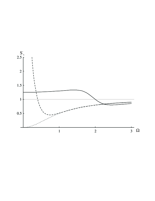
Figure 2: Intensity difference variance spectra as a function of the normalized frequency $\Omega$ for waveplate angles $\rho=0$ (dotted line), $\rho=0.01$, (dashed line) and $\rho=0.05$ (continuous line). Intracavity losses and output coupling coefficient, $(\mu,\,\kappa)=(0,0.05)$. The standard quantum limit is shown in grey. These plots are independent of $\sigma$.

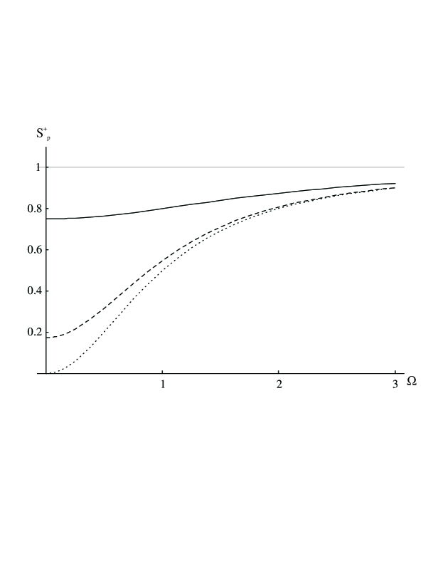
Figure 3: Phase sum variance spectra as a function of the normalized frequency $\Omega$ for normalized pump intensity $\sigma=1$ (dotted line), $\sigma=1.1$ (dashed line), $\sigma=2$ (continuous line). Intracavity losses and output coupling coefficient, $(\mu,\,\kappa)=(0,0.05)$. The standard quantum limit is shown in grey. These plots do not depend on the waveplate angle $\rho$.

These figures show that the amplitude quadrature difference variance goes to zero as $\rho$ goes to zero while the phase quadrature sum goes to zero close to threshold.

An important characteristic of the system is the minimal value obtained for $S^{-}_{x}$ as a function of $\Omega$, $\left(S^{-}_{x}\right)_{min}$ which is plotted in fig. 4 as a function of $\rho$.

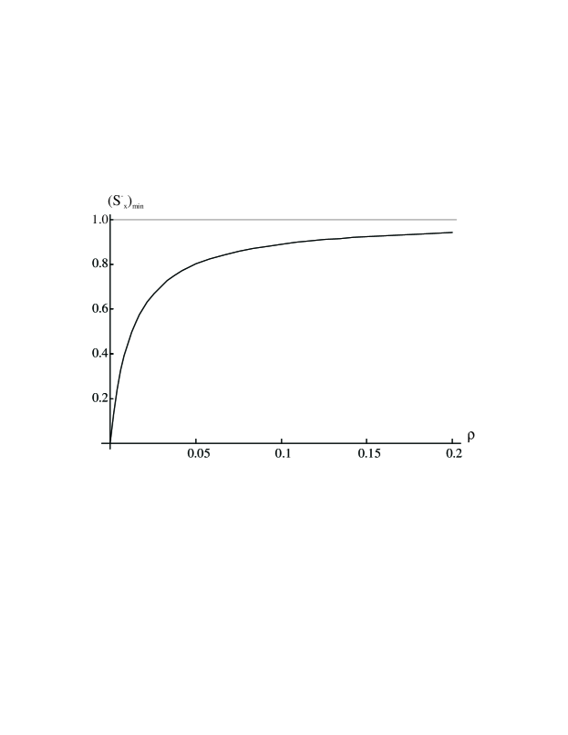
Figure 4: $\left(S^{-}_{x}\right)_{min}$ as a function of waveplate angle $\rho$ for intracavity losses and output coupling coefficient, $(\mu,\,\kappa)=(0,0.05)$. The standard quantum limit is shown in grey.

This plot shows that one obtains a significant noise reduction as long as $\rho$ is small compared to $\kappa$.

4 Entanglement criteria

4.1 EPR correlations criterion

In the Gedanken Experiment discussed in epr , one tries to infer the quantum state of a particle by measurements on a spatially separated particle : the optical equivalent of that scheme is to try to infer the signal beam by measurements on the spatially separated idler beam. In this case, quantum correlations do not suffice to characterize the efficiency of the system and another criterion has to be considered reid . The noise on the measured observable has to be taken into account : a large noise will reduce the precision with which the unmeasured system is known. One is lead to introduce inference errors or conditional variances reid . The conditional variances for amplitude and phase are given by :

$$V_{x} = \min_{g}\langle|\delta\tilde{x}_{1}-g\delta\tilde{x}_{2}|^{2}\rangle=\langle|\delta\tilde{x}_{1}-C_{x}\delta\tilde{x}_{2}|^{2}\rangle$$ (13)

$$V_{p} = \min_{g}\langle|\delta\tilde{p}_{1}-g\delta\tilde{p}_{2}|^{2}\rangle=\langle|\delta\tilde{p}_{1}-C_{p}\delta\tilde{p}_{2}|^{2}\rangle$$ (14)

where

$$C_{x} = \frac{\langle\delta\tilde{x}_{1}(\Omega)\delta\tilde{x}_{2}(-\Omega)\rangle}{\sqrt{\langle\delta\tilde{x}_{1}^{2}\rangle\langle\delta\tilde{x}_{2}^{2}\rangle}}$$ (15)

$$C_{p} = \frac{\langle\delta\tilde{p}_{1}(\Omega)\delta\tilde{p}_{2}(-\Omega)\rangle}{\sqrt{\langle\delta\tilde{p}_{1}^{2}\rangle\langle\delta\tilde{p}_{2}^{2}\rangle}}$$ (16)

are the normalized correlations. Ref. reid shows that one must have $V_{x}V_{p}<1$ in order to have a demonstration of the EPR paradox.

Even with correlations factors close but not equal to unity, the conditional variances can be large if the quantum noise on the individual beams is large as is the case for the amplitude quadrature.

The conditional variances $V_{x}$ and $V_{p}$ are shown on fig. 5 and 6. Due to the large excess noise on the amplitude quadrature at low frequencies, $V_{x}$ is large for low frequencies while $V_{p}$ remains low for all frequencies. This difference between the two conditional variances is one of the main differences between our case and the other devices which have been introduced to generate bright entangled beams eprbachor ; eprkimble ; eprtaiyuan ; eprpolzik : in these cases, one obtains theoretically symmetric behaviors for amplitude and phase which is not the case in our system.

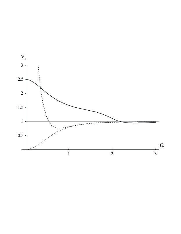
Figure 5: Conditional variance spectra for the amplitude quadrature $V_{x}$ as a function of the normalized frequency $\Omega$ for wave plate angle $\rho=0$ (dotted line), $\rho=0.01$, (dashed line) and $\rho=0.05$ (continuous line). Intracavity losses and output coupling coefficient, $(\mu,\,\kappa)=(0,0.05)$. The standard quantum limit is shown in grey. Normalized pump intensity $\sigma=1$.

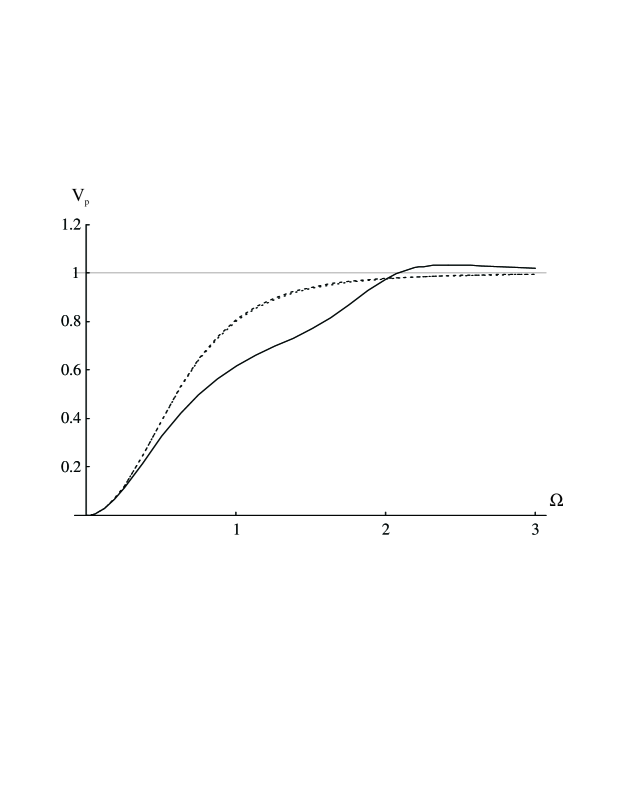
Figure 6: Conditional variance spectra for the phase quadrature $V_{p}$ as a function of the normalized frequency $\Omega$ for wave plate angle $\rho=0$ (dotted line), $\rho=0.01$, (dashed line) and $\rho=0.05$ (continuous line). The first two curves cannot be distinguished on the figure. Intracavity losses and output coupling coefficient, $(\mu,\,\kappa)=(0,0.05)$. The standard quantum limit is shown in grey. Normalized pump intensity $\sigma=1$.

The variation of $V_{x}V_{p}$ with $\Omega$ is plotted on fig. 7. This figure shows that EPR correlations exist in a broad frequency range even for large values of the waveplate angle. The behavior of the criterion is dominated by that of $V_{p}$ which goes to zero as $\Omega$ goes to zero and is independent of the waveplate angle.

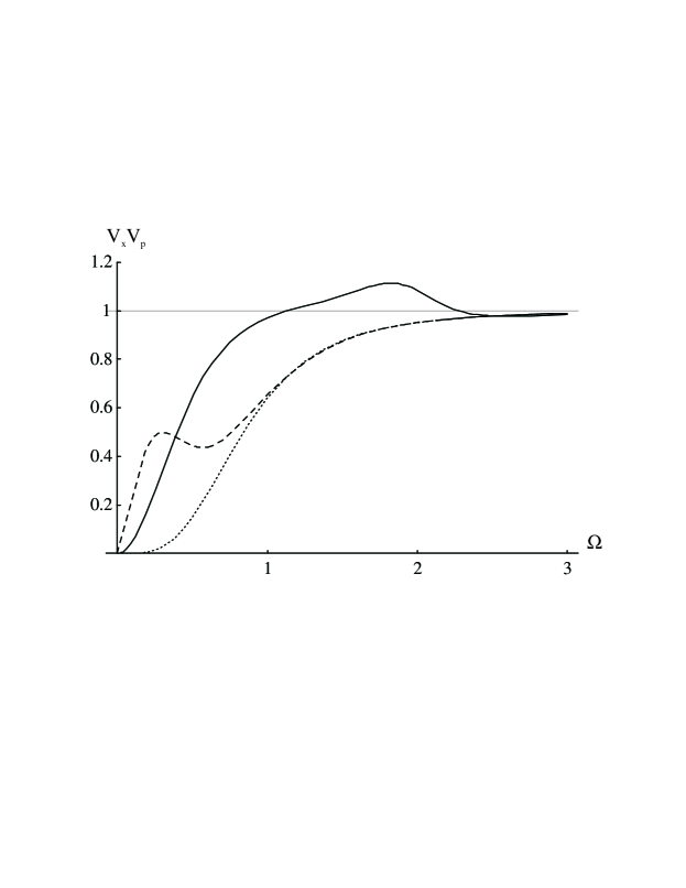
Figure 7: $V_{x}V_{p}$ as a function of $\Omega$ for intracavity losses and output coupling coefficient, $(\mu,\,\kappa)=(0,\,0.05)$ and for wave plate angle $\rho=0$ (dotted line), $\rho=0.01$, (dashed line) and $\rho=0.05$ (continuous line). The EPR correlations limit is shown in grey. Normalized pump intensity $\sigma=1$.

4.2 Inseparability criterion

However, this criterion is not always relevant. In the vast majority of quantum information protocols, what matters is the non-separability of the quantum state that is the impossibility to express it as a product of independent sub-states. In order to evaluate the inseparability of two systems, Peres proposed a necessary criterion which applies to finite dimension systems peres which was latter shown by Horodecki horodecki to be sufficient for dimensions smaller than $2\times 2$ - or $2\times 3$ -. In the particular case of Gaussian states, Duan et al. duan and Simon simon developed a necessary criterion for inseparability which can be written as :

$$S_{x}^{-}+S_{p}^{+}\leq 2$$ (17)

where $S_{x}^{-}$ and $S_{p}^{+}$ are the previously introduced variances spectra. Let us note the entanglement produced by the self-phase locked OPO is not in the so-called standard form (duan , equations 10-11) : in this case, the above criterion is a sufficient but not necessary condition for inseparability.

The value of $S_{x}^{-}+S_{p}^{+}$ as a function of $\Omega$ is plotted in fig 8. At low frequencies, the behavior is dominated by the behavior of $S_{x}^{-}$ which is large. As higher frequencies are considered, the figure shows that the system is indeed entangled over a large range of frequencies. When $\rho\ll\kappa$, the excess noise on the amplitude quadrature makes the sum larger than two meaning that the system is separable. The curves are plotted for a value $\sigma=1$, that is at exact threshold. Increasing $\sigma$ does not increase significantly the variance $S_{x}^{-}$ and does not modify $S_{p}^{+}$ and will thus move all the curves toward the inseparability limit while keeping the sum below two. It is the behavior of the amplitude fluctuations which dominates that of the sum of the variances.

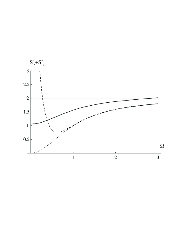
Figure 8: $S_{x}^{-}+S_{p}^{+}$ as a function of $\Omega$ for intracavity losses and output coupling coefficient $(\mu,\,\kappa)=(0,\,0.05)$ and wave plate angle $\rho=0$ (dotted line), $\rho=0.01$ (dashed line), $\rho=0.1$ (continuous line). The inseparability limit is shown in grey.

4.3 Fidelity of teleportation

In teleportation experiments, one tries to transfer quantum states from one point to another with a unity gain. In this case, the successful of the teleportation is characterized by the overlap between the input and output states. This overlap is usually called the fidelity teleportkimble . It can be shown that in order to obtain a fidelity larger than $1\over 2$, quantum correlations must be used, while a fidelity larger than $2\over 3$ denotes the possession by the receiver of the best copy available grangier . In the particular case of gaussian states, one can show that the fidelity is related to the intensity difference and phase sum variances defined in equation 10 by the relation :

$$\mathcal{F}=\frac{1}{\sqrt{(1+S^{-}_{x})(1+S^{+}_{p})}}$$ (18)

The fidelity as a function of the normalized frequency is shown in fig 9 for different angles of the waveplate.

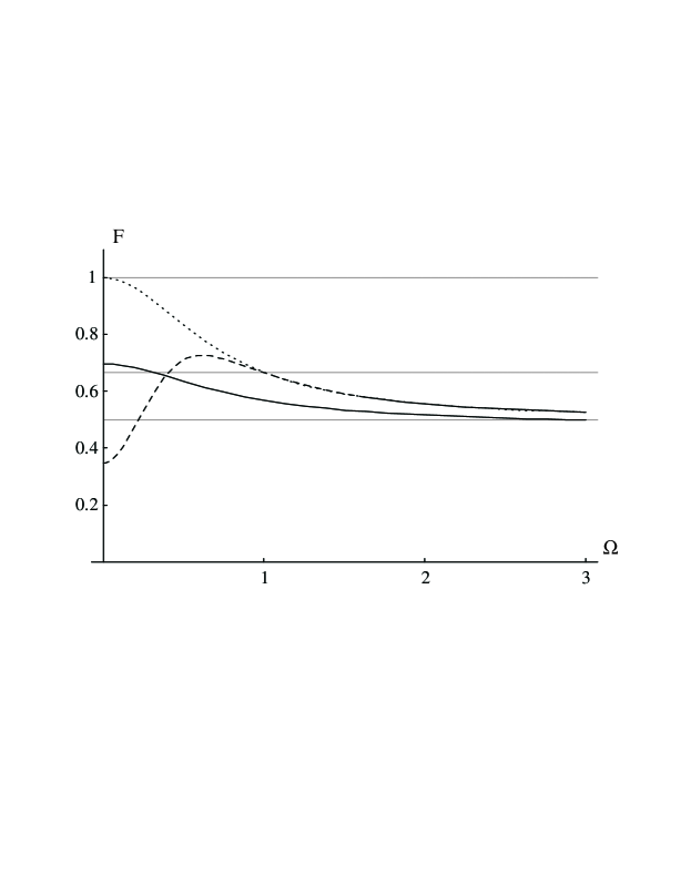
Figure 9: Fidelity, $\mathcal{F}$ as a function of analysis frequency $\Omega$ for intracavity losses and output coupling coefficient $(\mu,\,\kappa)=(0,\,0.05)$ and wave plate angle $\rho=0$ (dotted line), $\rho=0.01$ (dashed line), $\rho=0.1$ (continuous line). The grey lines correspond to perfect teleportation ($\mathcal{F}=1$), ”best copy” limit ($\mathcal{F}=2/3$) and classical limit ($\mathcal{F}=1/2$).

One sees that for small values of the waveplate angle $\rho$, one obtains a fidelity larger that the ”best copy” limit ($\mathcal{F}\geq 2/3$) over a large frequency range.

In order to determine the optimal operating parameters, one can plot the values of waveplate angle $\rho$, normalized intensity $\sigma$ and analysis frequency $\Omega$ for which the fidelity is equal to the ”best-copy” limit, that is $\mathcal{F}=\frac{2}{3}$. The plot consists of two zones : close to threshold, i.e. $\sigma<1.1$, one obtains a fidelity larger than $2\over 3$ for large values of $\rho$ and for $\Omega<0.5$ (dark grey surface) ; for $\sigma>1.1$, a large fidelity is observed over a larger range of frequencies but only for very small values of $\rho$, typically $\rho<0.02$ (light grey surface).

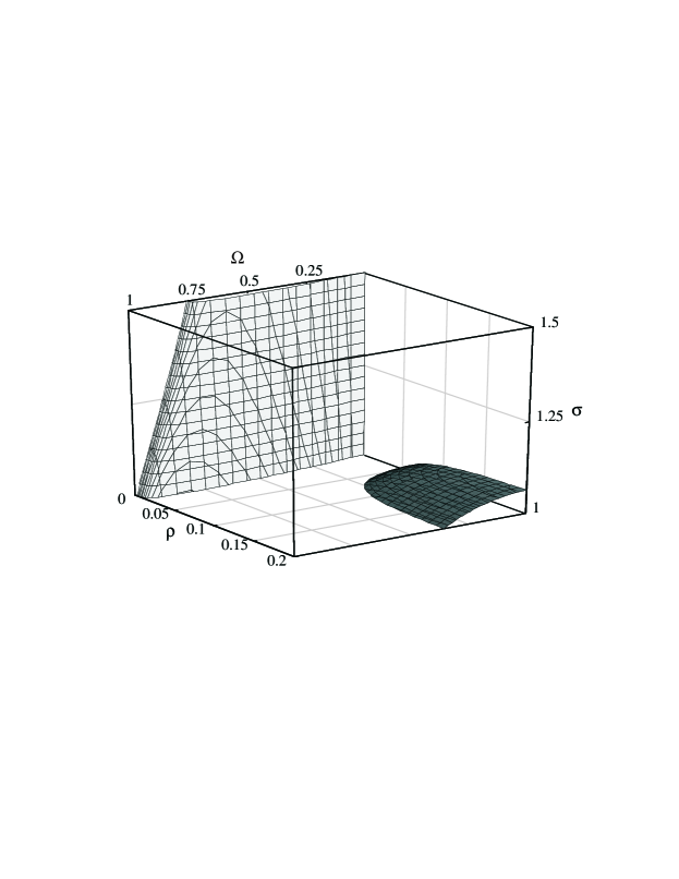
Figure 10: Values of the analysis frequency $\Omega$, wave plate angle $\rho$ and normalized pump intensity $\sigma$ for which $\mathcal{F}=\frac{2}{3}$. Intracavity losses and output coupling coefficient $(\mu,\,\kappa)=(0,\,0.1)$.

One observes that in order to obtain a fidelity significantly larger than $2\over 3$, one can use very small angles, typically less than $1^{\circ}$ (0.015 radians). As mentioned in ref. part1 , this is feasible experimentally, since a small angle does not reduce the range of the crystal temperature and cavity length where the locking is observed but only its total surface : once frequency degeneracy has been obtained, existing active stabilization of the system allows for operation in this zone. However, working very close to threshold will reduce the parameter range where phase locking is observed and may be difficult experimentally.

We have shown in this section that our system produces bright entangled beams which fulfill different entanglement criteria over a large range of frequencies. At low frequencies, the entanglement is observed for $\rho\ll\kappa$, that is for a rotation of the waveplate small compared to the mirror transmission.

5 Use of optimized quadratures

The limitation of the EPR correlations zone to small angle is due to the fact that the intensity correlations are no longer perfect in a phase locked OPO as was the case in the standard OPO. A simple picture shows the origin of this phenomenon. $A_{1}$ and $A_{2}$ having a fixed phase relation, the output beam is in a fixed polarization state which we denote $A_{bright}$. The orthogonal polarization mode has a zero mean value and is denoted $A_{dark}$. One can show that they correspond to the polarization eigenmodes of the ”cold” OPO, that is without the pump beam eigenmodes .

One can also show that their variance spectra are

$$\begin{array}[]{>{\displaystyle}c>{\displaystyle}c>{\displaystyle}c}S_{x}(A_{dark})&=&\left\langle|\delta\tilde{x}_{dark}|^{2}\right\rangle=\frac{1}{2}\left\langle|\delta\tilde{x}_{1}-\delta\tilde{x}_{2}|^{2}\right\rangle=S_{x}^{-}\\ S_{p}(A_{bright})&=&\left\langle|\delta\tilde{p}_{bright}|^{2}\right\rangle=\frac{1}{2}\left\langle|\delta\tilde{p}_{1}+\delta\tilde{p}_{2}|^{2}\right\rangle=S_{p}^{+}\end{array}$$ (19)

The exact expressions of the mean fields $A_{bright}$ and $A_{dark}$ depend on the choice of the operating point. For the minimum threshold point where we have performed our calculations, we have

$$A_{bright} = \frac{A_{1}+A_{2}}{\sqrt{2}}$$ (20)

$$A_{dark} = \frac{A_{1}-A_{2}}{\sqrt{2}}$$ (21)

which are left and right circularly polarized due to the $\pi\over 2$ phase shift between $A_{1}$ and $A_{2}$.

As we have seen previously that $S_{x}^{-}$ and $S_{p}^{+}$ can be smaller than the corresponding standard quantum limit, $A_{bright}$ is phase squeezed while $A_{dark}$ is squeezed on the orthogonal quadrature. This is shown in fig. 11 which represents the Fresnel diagram common to the fields $A_{1}$, $A_{2}$, $A_{bright}$ and $A_{dark}$, the phase reference being the phase of the field $A_{bright}$.

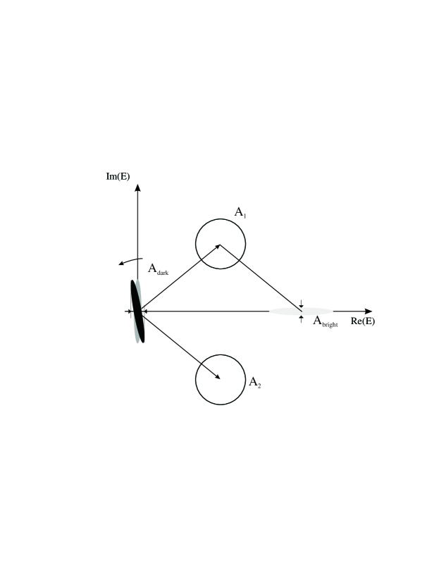
Figure 11: Fresnel picture of the signal and idler (white surfaces), $A_{bright}$ (light grey) and $A_{dark}$ fields in the case of a standard OPO (black) and in the case of a phase locked OPO (dark grey).

The increase in $S_{x}^{-}$ at low frequencies corresponds to to the tilt of the corresponding squeezing ellipse (in black) with respect to the standard OPO situation (vertical ellipse in dark grey). Due to the presence of the waveplate, the amplitude quadrature of $A_{dark}$ (measurement of the width along the horizontal axis) is not the optimal quadrature : it is thus natural to detect this optimal quadrature instead of the amplitude quadraturejosse . It is possible to dephase appropriately $A_{1}$ with respect to $A_{2}$ so that $A_{bright}$ and $A_{dark}$ are now squeezed on orthogonal quadratures. In the simple case of the minimum threshold point, the new entangled are simply obtained by a linear superposition of the original fields along the neutral axis of the crystal. In the simple case of the minimum threshold point, these fields are given by :

$$A^{\prime}_{1} = \frac{1}{\sqrt{2}}\left[\cos\left(\frac{\theta_{opt}}{2}\right)A_{1}-i\sin\left(\frac{\theta_{opt}}{2}\right)A_{2}\right]$$ (22)

$$A^{\prime}_{2} = \frac{1}{\sqrt{2}}\left[\sin\left(\frac{\theta_{opt}}{2}\right)A_{1}+i\cos\left(\frac{\theta_{opt}}{2}\right)A_{2}\right]$$ (23)

where $\theta_{opt}$ is given by :

$$\theta_{opt}=\frac{1}{2}\mathrm{arctan}\left(\frac{2C_{-}\sqrt{S_{x}\left(A_{dark}\right)S_{p}\left(A_{dark}\right)}}{S_{x}\left(A_{dark}\right)-S_{p}\left(A_{dark}\right)}\right)$$ (24)

and

$$C_{-}=\frac{\left\langle\delta\tilde{x}\left(A_{dark}\right)\delta\tilde{p}\left(A_{dark}\right)\right\rangle}{\sqrt{S_{x}\left(A_{dark}\right)S_{p}\left(A_{dark}\right)}}$$ (25)

The inseparability criterion developed by Duan et al. duan is

$$S_{x}^{+}\left(A^{\prime}_{bright}+\right)+S_{p}\left(A^{\prime}_{dark}\right)\leq 2$$ (26)

where $S_{x,p}\left(A_{bright,dark}\right)$ are defined above and $A^{\prime}_{bright,dark}$ are the optimally squeezed states :

$$A^{\prime}_{bright,dark}=\frac{A^{\prime}_{1}\pm A^{\prime}_{2}}{\sqrt{2}}$$ (27)

Setting $\rho$ and $\sigma$, one can plot $S_{p}\left(A^{\prime}_{bright}\right)+S_{x}\left(A^{\prime}_{dark}\right)$ as a function of the frequency (figure 12). This figure shows that one can obtain a much larger violation of the inseparability criterion using optimized quadratures. For $\rho=0.01~{}\mbox{rad}$, the value obtained is very close to the curve obtained for a standard OPO (where frequency non degeneracy and phase diffusion prevent the measurement). Furthermore, the divergence obtained at low frequencies is completely eliminated. For larger values of the waveplate angle, the improvement is still noticeable.

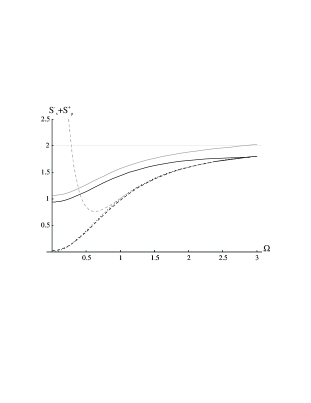
Figure 12: $S_{p}\left(A^{\prime}_{bright}\right)+S_{x}\left(A^{\prime}_{dark}\right)$ as a function of analysis frequency $\Omega$ for intracavity losses and output coupling coefficient $(\mu,\,\kappa)=(0,\,0.05)$ and waveplate angle $\rho=0$ (dotted line), $\rho=0.01$ (dashed line), $\rho=0.05$ (continuous line). Grey lines correspond to the curves obtained on fig. 8 for $S_{p}^{+}+S_{x}^{-}$

6 Conclusion

We have shown that a type II OPO containing a birefringent element can be a very efficient source of intense entangled beams. This entanglement has been characterized by the use of several criteria, namely intensity difference and phase sum variances, inference errors which denote the possibility to make an EPR-type Gedanken Experiment, inseparability criteria which correspond to the quality of the entanglement and fidelity which represent the quality of teleportation with unity gain. These criteria have been shown to be fulfilled for a large range of operating parameters thus showing the quality of the system. The inseparability criterion can be largely improved by the use of optimized quadratures. We are currently setting up an experiment based on this system.

References

- (1) A. Furusawa, J.L. Sorensen, S.L. Braunstein, C.A. Fuchs, H.J. Kimble, E.S. Polzik, Science 282 (1998) 706.
- (2) F. Grosshans and P. Grangier, Phys. Rev. A 64, 010301 (2001)
- (3) Ch. Silberhorn, P.K. Lam, O. Weiß, F. König, N. Korolkova and G. Leuchs, Phys. Rev. Lett. 86, 4267 (2001).
- (4) A. Einstein, B. Podolski and N. Rosen, Phys. Rev 47, (1935) 777.
- (5) W.P. Bowen, N. Treps, B.C. Buchler, R. Schnabel, T.C. Ralph, H. Bachor, T. Symul, and P.K. Lam, Phys. Rev. A 67, 032302 (2003)
- (6) Z.Y Ou, S.F. Pereira, H.J Kimble, K.C. Peng, Phys. Rev. Lett 68, 3663 (1992).
- (7) Zhang, Y. et al., Phys. Rev. A 62, 023813 (2000)
- (8) C. Schori, J.L. Sorensen, E.S. Polzik, Phys. Rev. A 66 033802 (2002)
- (9) Peng, K. C. et al., Appl. Phys. B 66, 755 (1998).
- (10) Ling-An Wu, H.J. Kimble, J. L. Hall, and Huifa Wu, Phys. Rev. Lett 57, 2520 (1986).
- (11) J. Mertz, T. Debuisschert, A. Heidmann, Fabre, E. Giacobino, Opt. Lett. 16, 1234 (1991).
- (12) K. Schneider, R. Bruckmeier, H. Hansen, S. Schiller, J. Mlynek, Opt. lett. 21, 1396 (1996).
- (13) K.S. Zhang, M. Martinelli, T. Coudreau, A. Maître, C. Fabre, J. Opt A : Quant. and Semiclass. Opt. 3 (2001).
- (14) J. Laurat, T. Coudreau, N. Treps, A. Maître, C. Fabre, Phys. Rev. Lett. 91 213601 (2003).
- (15) S. Reynaud, C. Fabre, E. Giacobino, J. Opt. Soc. Am. B 4, 1520 (1987).
- (16) S. Feng and O. Pfister, J. Opt. B:Quantum Semiclass. Opt. 5, 262 (2003).
- (17) J.-Y. Courtois, A. Smith, C. Fabre, S. Reynaud, J. Mod. Opt. 38, 177 (1991).
- (18) E.J. Mason, N.C. Wong, Opt. Lett. 23, 1733 (1998).
- (19) C. Fabre, E.J. Mason, N.C. Wong, Optics Comm. 170, 299 (1999).
- (20) L. Longchambon, J. Laurat, T. Coudreau, C. Fabre, submitted to EPJD, quant/ph 0310036.
- (21) M.D Reid, Phys. Rev. A 40, 913 (1989).
- (22) A. Peres, Phys. Rev. Lett 77, 1413 (1996).
- (23) P. Horodecki, Phys. Lett. A 232, 333 (1997).
- (24) Lu-Ming Duan, G. Giedke, J. I. Cirac, and P. Zoller, Phys. Rev. Lett 84, 2722 (2000).
- (25) R. Simon, Phys. Rev. Lett 84, 2726 (2000).
- (26) C. Fabre, E. Giacobino, A. Heidmann, L. Lugiato, S. Reynaud, M. Vadacchino, Wang Kaige, Quantum Opt. 2, 159 (1990).
- (27) L. Longchambon, J. Laurat, T. Coudreau, C. Fabre, in preparation.
- (28) V. Josse, A. Dantan, A. Bramati, E. Giacobino, accepted in J. Opt. B - Special Issue on Foundations of Quantum Optics, e-print quant-ph/0310139