Quantum and classical correlations between players in game theory

Abstract

Effects of quantum and classical correlations on game theory are studied to clarify the new aspects brought into game theory by the quantum mechanical toolbox. In this study, we compare quantum correlation represented by a maximally entangled state and classical correlation that is generated through phase damping processes on the maximally entangled state. Thus, this also sheds light on the behavior of games under the influence of noisy sources. It is observed that the quantum correlation can always resolve the dilemmas in non-zero sum games and attain the maximum sum of both players’ payoffs, while the classical correlation cannot necessarily resolve the dilemmas.

I Introduction

Recently, there has been a growing interest in game theory within the quantum information community Eisert1 ; Meyer . The concepts of quantum mechanics have been introduced to study quantum versions of classical game theory. This new version, which is referred to as Quantum Game Theory, can exploit quantum superpositions, entanglement, and quantum operations that are absent from classical game theory. So far, researches on the quantum versions of game theory have focused mainly on observing the dynamics and outcomes of games in the quantum domain. One of the motivations of introducing quantum mechanics into game theory is to find a solution resolving the dilemmas in the games, which cannot be achieved in classical game theory. Another one is that the study of quantum versions of game theory might be useful to examine many complicated and open problems in quantum information science.

Most of the studies that have been conducted so far are devoted to resolving the dilemmas inherit in classical games with the help of quantum mechanics. In fact, they have been resolved by using entanglement. In the course of the research, however, we come up with the question: Is entanglement really essential to resolve the dilemmas in the games ? In other words, can classical correlations replace quantum ones (entanglement) to obtain similar results ? If entanglement turns out to be inessential, it is natural to ask what the difference in payoffs depending on the types of correlations is.

Our purpose in this study is to make a comparative analysis of the effects of shared quantum and classical correlations on the strategies of players and on the dynamics of games. In particular, we would like to focus on whether classical correlations can produce the same results as that of quantum correlations. Even if they cannot, it is worth investigating to what extent classical correlations can enhance original classical games. In this study, we consider the following games: Prisoner’s Dilemma (PD), Chicken Game (CG), Stag Hunt (SH), Battle of Sexes (BoS), Matching Penny (MP), Samaritan’s Dilemma (SD), and the Monty Hall game (MH). All of these games have different types of dilemmas and they fall into different classes when they are classified according to their classical payoff matrices. All but MH, which is a sequential game, are 2$\times$2 strategic games (see Ref. Rasmusen for details of these games).

II Classical game theory

In this section we will briefly describe the rules of classical game theory and introduce several games studied in this paper. A strategic game can be denoted by $\Gamma=[N,(S_{i})_{i\in N},(u_{i})_{i\in N}]$ where $N$ is the set of players, $S_{i}$ is the set of strategies for the $i$-th player, and $u_{i}$ is the payoff function for the $i$-th player, which is a map from the set of all possible strategy combinations into real numbers myerson . Then the payoff for the $i$-th player can be denoted as $u_{i}(s)$ where $s$ is a combination of the strategies implemented by all players. In classical game theory, any strategic game is fully described by its payoff matrix. For 2$\times$2 strategic games, the properties of the games are determined by each player’s four possible payoffs. The payoff matrices of the strategic games we discuss are shown in Fig.1(a). 2$\times$2 games can be classified into 78 types, provided that all the four possible payoffs for each player are different Rapop . We will deal with only games that have dilemmas, while most of these 78 different types do not have dilemmas.

According to the above classification into 78 types, there are only four symmetric games with a dilemma which arises from the incentive not to cooperate. These four games are PD, CG, SH, and Deadlock game poundstone . In the last one, players do not face the problem of choosing the strategy because players can decide on a unique Nash equilibria (NE) without hesitation in the sense that they do not have any incentive to deviate from the NE. On the other hand, for PD and SH, there exist incentives to deviate from an NE from mathematical or psychological motivation. For CG, since there exist two equivalent NE’s, players cannot decide on which NE to choose.

Next, we will briefly mention the nature of the dilemma in each game. As it can be seen from the tables, PD has one NE where both players get the payoff $\gamma$ when they both choose to play “defect” (D). On the other hand, when both play “cooperate” (C), they get the payoff $\beta$ corresponding to Pareto optimal. Here the dilemma occurs because Pareto optimal and the NE of the game do not coincide.

The type of the dilemma in CG is different from that in PD. In CG, the dilemma occurs because there exist two NE’s with the payoffs $(\alpha,\gamma)$ and $(\gamma,\alpha)$ at the strategy sets (C,S) and (S,C) where S and C stand for “swerve” and “continue”, respectively. Therefore, the players without communicating with each other cannot decide on which NE to choose.

The type of the dilemma in SH is very different from those in the above two games. SH has two NE’s at which both players go for a “stag” (S) or go for a “rabbit” (R). Obviously, going for a “stag” is the best strategy for both players. For PD and CG, games are discussed on the assumption that players are rational, on which there exists no dilemma in SH. However, in this game, the dilemma can be found in the following sense: If one goes for a stag but the other player goes for a rabbit, then the former get the worst possible payoff $\delta$, while the latter still get the second highest payoff $\beta$. In other words, the dilemma arises from the fear that the other player might not be rational. This type of the dilemma can often be seen in society poundstone .

Having shown the dilemmas in symmetric games, we will explain asymmetric games below. BoS has a dilemma similar to that in CG. The NE’s are at (O,O) and (F,F) where O is the choice of going to “opera” and F is the choice of going to a “football match”. The difference between BoS and CG is that the former has an asymmetric payoff matrix, whereas the latter has a symmetric one. BoS and the three games mentioned above have at least one NE.

MP is different from the above four games, not only because it is a zero sum game, but also because it is a discoordination game Rasmusen , i.e., there is no NE in the original classical game. Since the interests of players conflict, they will never try to coordinate their strategies of playing “head” (H) or “tail” (T).

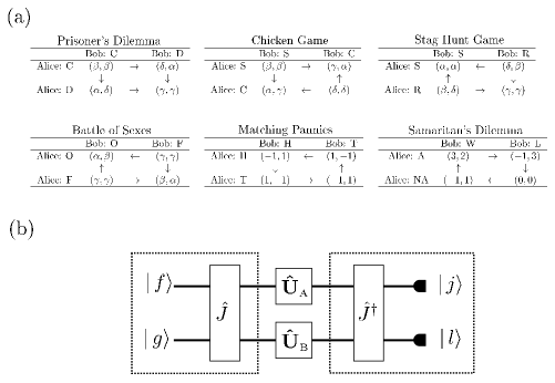
Figure 1: (a) Payoff matrices for games in this study where $\alpha>\beta>\gamma>\delta$ and $2\beta>\alpha+\delta$ for symmetric games. Additional conditions $\alpha+\delta>\beta+\gamma$ for PD, $\alpha+\delta=\beta+\gamma$ for CG, and $\alpha+\delta>\beta+\gamma$ for SH are imposed. Arrows show the best response of a player to a fixed choice of the other player. Any strategy pointed by two arrows is an NE. (b) Schematic configuration of the quantization scheme for $2\times 2$ strategic games. The operations inside the dotted boxes are performed by the referee.

This game is also classified as an asymmetric game.

SD is also a discoordination and asymmetric game but not a zero sum game. It is seen from the table that there is no NE in the pure strategies. When the players adopt classical mixed strategies, a unique NE is realized when Alice chooses “aid” (A) with probability 0.5 and Bob chooses “work” (W) with probability 0.25. Although the classical mixed strategy gives the unique NE, Alice’s payoff is negative. This is the dilemma in the game, which corresponds to the fact that Alice, who likes to help the person in need (Bob) voluntarily, is exploited by the selfish behavior of Bob and she cannot stop this exploitation. In the classical mixed strategies, the payoff of Alice and Bob are -0.25 and 1.5, respectively, where there still remains the dilemma for Alice because her payoff is negative, implying her loss of resources.

MH is classified as a sequential game monty . The scenario is as follows: The participant (Bob) is given the opportunity to select one out of three closed doors, behind one of which there is a prize. There is no prize behind the other two doors. Once he makes his choice, Monty Hall (Alice) will open one of the remaining doors, revealing that it does not contain the prize. She then asks him if he would like to switch his choice to the other unopened door, or stay with his original choice. Can he increase the probability of wining the prize by changing his choice ? MH attracted much interest because the answer is counterintuitive. Classically, the best strategy for Bob is to switch his choice, which doubles the chance of wining the prize.

III Scheme for the quantum version of $2\times 2$ games

III.1 Quantum operations (QO) and quantum correlation (QC)

We will introduce the scheme for a quantum version of these games. A quantum version of a 2$\times$2 classical game with a maximally entangled state shared between the players is played as follows Eisert1 [see Fig.1 (b)]: (a) A referee prepares a maximally entangled state by applying an entangling operator $\hat{J}$ on a product state $|\,f\rangle|\,g\rangle$ where $\hat{J}$ is defined as $\hat{J}|\,f\rangle|\,g\rangle=\frac{1}{\sqrt{2}}\left[|\,f\rangle|\,g\rangle+i(-1)^{(f+g)}|\,(1-f)\rangle|\,(1-g)\rangle\right]$ with $f,g=0,1$. The output of this entangler $\rho_{in}=\hat{J}|\,fg\rangle\langle fg\,|\hat{J}^{\dagger}$ is delivered to the players. (b) The players apply their actions, which are SU(2) operators, locally on their qubits, and return the resultant state $\rho_{out}=(\hat{U}_{A}\otimes\hat{U}_{B})\rho_{in}(\hat{U}^{\dagger}_{A}\otimes\hat{U}^{\dagger}_{B})$ to the referee. Alice’s and Bob’s actions are restricted to the two-parameter SU(2) operators, $\hat{U}_{A}(\theta_{A},\phi_{A})$ and $\hat{U}_{B}(\theta_{B},\phi_{B})$, given as

$$\hat{U}(\theta,\phi)=\left(\begin{array}[]{cc}e^{i\phi}\cos\frac{\theta}{2}&\sin\frac{\theta}{2}\\ \sin\frac{\theta}{2}&e^{-i\phi}\cos\frac{\theta}{2}\end{array}\right),$$ (1)

with $0\leq\phi\leq\pi/2$ and $0\leq\theta\leq\pi$. In particular, the identity operator ($\hat{\sigma}_{0}$) and the bit flip operator ($i\hat{\sigma}_{y}$) correspond to the two classical pure strategies. (c) The referee, upon receiving this state, applies $\hat{J}^{\dagger}$ and then makes a measurement $\{\Pi_{n}=|\,jl\rangle\langle jl\,|\}_{\{{j,l}={0,1}\}}$ with $n=2j+l$. According to the measurement outcome $n$, the referee assigns each player the payoff chosen from the payoff matrix of the original classical game. Then the average payoff of the players can be written as $\$_{A}=\sum_{n}a_{n}\rm{Tr}(\Pi_{n}\it{\hat{J}}^{\dagger}\hat{\rho}_{\rm{out}}\hat{J}),\$_{B}=\sum_{n}b_{n}\rm{Tr}(\Pi_{n}\it{\hat{J}}^{\dagger}\hat{\rho}_{\rm{out}}\hat{J})$ where $a_{n}$ and $b_{n}$ are the payoffs chosen from the classical payoff matrix when the measurement result is $n$.

When an input state is $|\,f\rangle|\,g\rangle=|\,0\rangle|\,0\rangle$, the probabilities of obtaining $n=2j+l$, $P_{jl}$’s, are given by

$$P_{00} = |\,\cos(\theta_{A}/2)\cos(\theta_{B}/2)\cos(\phi_{A}+\phi_{B})\,|^{2},$$

$$P_{01} = |\,x\sin\phi_{B}-y\cos\phi_{A}\,|^{2},$$

$$P_{10} = |\,x\cos\phi_{B}-y\sin\phi_{A}\,|^{2},$$

$$P_{11} = |\,\sin(\theta_{A}/2)\sin(\theta_{B}/2)+\cos(\theta_{A}/2)\cos(\theta_{B}/2)\sin(\phi_{A}+\phi_{B})\,|^{2},$$ (2)

where $x=\sin(\theta_{A}/2)\cos(\theta_{B}/2)$ and $y=\cos(\theta_{A}/2)\sin(\theta_{B}/2)$.

III.2 Quantum operations (QO) and classical correlation (CC)

Here we assume that the players are allowed to use quantum operations as shown in Eq.(1), however, the shared state is a classically correlated state of the form $\rho^{\prime}=\frac{1}{2}[|\,00\rangle\langle 00\,|+|\,11\rangle\langle 11\,|]$. This can occur, for example, when the maximally entangled state generated by the referee undergoes a damping process where the off-diagonal elements of the density operator disappear. Thus the game with a shared classical correlation proceeds as in the preceding subsection with $\rho_{in}$ replaced by a classically correlated state $\rho^{\prime}$.

When $\rho^{\prime}=\frac{1}{2}[|\,00\rangle\langle 00\,|+|\,11\rangle\langle 11\,|]$, the probabilities of obtaining $n=2j+l$, $P_{jl}$’s, are given by

$$P_{00} = \frac{1}{4}[1+\cos\theta_{A}\cos\theta_{B}-\sin\theta_{A}\sin\theta_{B}\sin(\phi_{A}+\phi_{B})],$$

$$P_{01} = \frac{1}{4}[1-\cos\theta_{A}\cos\theta_{B}+\sin\theta_{A}\sin\theta_{B}\sin(\phi_{A}-\phi_{B})],$$

$$P_{10} = \frac{1}{4}[1-\cos\theta_{A}\cos\theta_{B}-\sin\theta_{A}\sin\theta_{B}\sin(\phi_{A}-\phi_{B})],$$

$$P_{11} = \frac{1}{4}[1+\cos\theta_{A}\cos\theta_{B}+\sin\theta_{A}\sin\theta_{B}\sin(\phi_{A}+\phi_{B})].$$ (3)

IV Effects of shared quantum and classical correlations on the dynamics of the strategic games

In this section, we make a comparative analysis of the effects of shared quantum and classical correlations on the various types of games: (i) symmetric, non-zero sum game, (ii) asymmetric, non-zero sum game, (iii) asymmetric, zero sum, discoordination game, and (iv) asymmetric, non-zero sum, discoordination game.

IV.1 Symmetric, Non-zero sum game (PD, CG, SH)

In symmetric games, payoff functions are symmetric, which means Bob’s payoff can be calculated from the payoff function of Alice by interchanging Alice’s and Bob’s strategies. In PD, Alice’s payoff is given by

$$\$_{A} = \alpha P_{10}+\beta P_{00}+\gamma P_{11}+\delta P_{01}$$ (4)

$$= (\alpha-\delta)P_{10}+(\beta-\delta)P_{00}+(\gamma-\delta)P_{11}+\delta.$$

For CG, her payoff can be obtained as in Eq. (4) by interchanging $\gamma$ and $\delta$. For SH, her payoff is given as in Eq. (4) by interchanging $\alpha$ and $\beta$.

QO with QC: When PD is played with a shared quantum correlation, it has already been known that the strategy $(\hat{U}_{A}=i\hat{\sigma}_{z},\hat{U}_{B}=i\hat{\sigma}_{z})$ gives the payoff $(\$_{A},\$_{B})=(3,3)$ which coincides with Pareto optimal Eisert1 . Thus, the dilemma in this game is resolved. In CG, the coefficient of $P_{10}$ in Alice’s payoff is greater than the others and thus the same argument as in PD can be applied. The strategy $(\hat{U}_{A}=i\hat{\sigma}_{z},\hat{U}_{B}=i\hat{\sigma}_{z})$ gives a unique NE and can resolve the dilemma. For SH, there exist two equivalent NE’s with payoffs $(\$_{A},\$_{B})=(\alpha,\alpha)$ where $(\hat{U}_{A}=\hat{\sigma}_{0},\hat{U}_{B}=\hat{\sigma}_{0})$ or $(\hat{U}_{A}=i\hat{\sigma}_{z},\hat{U}_{B}=i\hat{\sigma}_{z})$. The dilemma in SH comes from the fear that if one chases a stag and the other chases a rabbit, the former cannot get anything. The former strategy corresponds to (S,S), however this cannot resolve the fear, i.e., if one player choose $i\hat{\sigma}_{y}$ (R), the other get the worst possible payoff, $\delta$. On the other hand, the latter strategy realizes an NE with the best possible payoffs for both players. Furthermore it guarantees a player choosing the strategy $i\hat{\sigma}_{z}$ at least the second lowest payoff $\gamma$, whatever strategy the other player chooses. It follows that the strategy $(\hat{U}_{A}=i\hat{\sigma}_{z},\hat{U}_{B}=i\hat{\sigma}_{z})$ is the best for the players and it resolves the dilemma in this game. Consequently, it turns out that quantum correlations and quantum operations can resolve the dilemma of “Symmetric, Non-zero sum games” with the same strategy, $\hat{U}_{A}=\hat{U}_{B}=i\hat{\sigma}_{z}$.

QO with CC: We analyze the effects of the classical correlations on the dynamics of the games. Let us begin with PD, in which Alice’s payoff is given by

$$\$_{A} = \frac{1}{4}[(\alpha+\beta+\gamma+\delta)+(-\alpha+\beta+\gamma-\delta)\cos\theta_{A}\cos\theta_{B}$$ (5)

$$+\sin\theta_{A}\sin\theta_{B}\{(-\alpha-\beta+\gamma+\delta)\sin\phi_{A}\cos\phi_{B}$$

$$+(\alpha-\beta+\gamma-\delta)\cos\phi_{A}\sin\phi_{B}\}].$$

Here, we impose the condition $\alpha+\delta>\beta+\gamma$, which is common to the conventional payoff matrices of PD with specific values. The analysis reveals the existence of three NE’s, two of which give the same amount of payoffs while the third NE gives much smaller payoff to the players. The two NE’s with equal payoffs emerge at $(\theta_{A}=0,\forall\phi_{A},\hat{U}_{B}=i\hat{\sigma}_{y})$ and $(\hat{U}_{A}=i\hat{\sigma}_{y},\theta_{B}=0,\forall\phi_{B})$. The other NE with a smaller payoff appears at $(\theta_{A}=\pi/2,\forall\phi_{A},\theta_{B}=\pi/2,\forall\phi_{B})$. In CG, we impose the condition $\alpha+\delta=\beta+\gamma$, which is common to the conventional payoff matrices of CG with specific values. The situation remains the same as PD except for the strategy that realizes the third NE. Thus, the dilemma cannot be resolved in this case as well. In SH, there exist three NE’s which are the same as those in PD; therefore the dilemma cannot be resolved due to the existence of two NE’s giving the same payoffs. Consequently, it follows that classical correlations cannot realize any NE achieved by quantum correlations and thus cannot resolve the dilemma. In the case of classical correlations, the main obstacle is the existence of two NE’s with the same payoff. Therefore, the players cannot decide on which NE to choose.

IV.2 Asymmetric, Non-zero sum game (BoS)

In this game, Alice’s payoff is given as

$$\$_{A} = \alpha P_{00}+\beta P_{11}+\gamma(P_{01}+P_{10})=(\alpha-\gamma)P_{00}+(\beta-\gamma)P_{11}+\gamma,$$ (6)

from which Bob’s payoff can be obtained by interchanging $\alpha$ and $\beta$.

QO with QC: In BoS, classical mixed strategies where Alice and Bob chooses “O” with probabilities $(\frac{\alpha-\gamma}{\alpha+\beta-2\gamma},\frac{\beta-\gamma}{\alpha+\beta-2\gamma})$ or $(\frac{\beta-\gamma}{\alpha+\beta-2\gamma},\frac{\alpha-\gamma}{\alpha+\beta-2\gamma})$ give NE’s with payoff $(\$_{A},\$_{B})=(\frac{\alpha\beta-\gamma}{\alpha+\beta-2\gamma},\frac{\alpha\beta-\gamma}{\alpha+\beta-2\gamma})$. On the other hand, using QO with QC, the players have infinite number of strategies resulting in infinite number of NE’s with the same payoff $(\$_{A},\$_{B})=(\beta-\gamma,\alpha-\gamma)$ where $(\theta_{A}=\theta_{B},\phi_{A}=\frac{\pi}{2}-\phi_{B})$ and $(\hat{U}_{A}=i\hat{\sigma}_{y},\hat{U}_{B}=i\hat{\sigma}_{y})$. Since the payoffs are all equal in the NE’s, the players cannot decide on which one to choose. But the concept of the focal point effect Rasmusen helps the players resolve the dilemma. The strategy $(\hat{U}_{A}=i\hat{\sigma}_{y},\hat{U}_{B}=i\hat{\sigma}_{y})$ is distinguished from other strategies because the players do not have to be concerned with the choice of the phase factor. Bob’s payoff is higher than Alice’s at all of these NE’s. This is an NE with unbalanced payoffs for Alice and Bob. While this unbalanced situation obtained when $|\,f\rangle|\,g\rangle=|\,0\rangle|\,0\rangle$ is favorable for Bob, one can easily show that if they start with $|\,f\rangle|\,g\rangle=|\,1\rangle|\,1\rangle$, this unbalanced situation will be favorable for Alice, that is, her payoff will be higher than Bob’s. This simple example shows the dependence of players’ payoffs on the input state.

QO with CC: In this case, we find two NE’s given by $(\theta_{A}=0,\forall\phi_{A},\theta_{B}=0,\forall\phi_{B})$ and $(\hat{U}_{A}=i\hat{\sigma}_{y},\hat{U}_{B}=i\hat{\sigma}_{y})$ with the same payoffs $(\$_{A},\$_{B})=((\alpha+\beta)/2,(\alpha+\beta)/2)$. The players, however, cannot decide on which NE’s to choose and thus the dilemma cannot be resolved. As a result, one can say that in this type of games, quantum correlations can achieve the unique NE with the help of the concept of the focal point, while classical correlations cannot.

IV.3 Asymmetric, Zero sum, Discoordination game (MP)

For MP, Alice’s payoff is given by

$$\$_{A} = -P_{00}-P_{11}+P_{01}+P_{10}=1-2(P_{00}+P_{11}).$$ (7)

Since this is a zero sum game, Bob’s payoff is obtained as $\$_{B}=-\$_{A}$ . Note that, in zero sum games, it is not the purpose of the players to find an equilibrium point on which they can compromise but rather to win the game and beat the other player. A straightforward calculation reveals that the players cannot find an equilibrium point when they use quantum operations and quantum correlation. On the other hand, when they play the game with quantum operations and classical correlation, there emerge NE’s with equal payoffs $(\$_{A},\$_{B})=(0,0)$ when the players apply the operators $(\theta_{A}=\frac{\pi}{2},\forall\phi_{A},\theta_{B}=\frac{\pi}{2},\forall\phi_{B})$. In this case, there is no winner and loser in the game. The payoffs they receive are equal to those they receive when they play the game with classical mixed strategies without any shared correlation.

IV.4 Asymmetric, Non-zero sum, Discoordination game (SD)

Alice’s and Bob’s payoffs in SD are given by,

$$\$_{A} = 3P_{00}-P_{01}-P_{10},$$

$$\$_{B} = 2P_{00}+3P_{01}+P_{10}.$$ (8)

QO with QC: Our analysis reveals that there is the unique NE with the payoff given as $(3,2)$ where $(\hat{U}_{A}=i\hat{\sigma}_{z},\hat{U}_{B}=i\hat{\sigma}_{z})$. Introducing quantum operations and quantum correlation results in the emergence of the unique NE which cannot be seen in classical strategies. Both players receive higher payoffs than those obtained when a classical mixed strategy is applied. Note that, in classical mixed strategies, payoffs of the players are $(-0.2,1.5)$, which is much smaller than that obtained with QO and QC.

QO with CC: We found that there appears a unique NE with the payoff $(0.25,1.5)$ when the players apply $(\forall\theta_{A},\phi_{A}=0,\hat{U}_{B}=\frac{1}{\sqrt{2}}(\hat{\sigma}_{0}+i\hat{\sigma}_{y}))$. The payoff for Alice becomes greater than that of the classical mixed strategy while Bob’s remains unchanged.

Since Alice’s payoff $\$_{A}$ becomes positive in both cases with quantum and classical correlations, the dilemma in this game is successfully resolved. However, if we impose the further condition, $\$_{A}>\$_{B}$, then it can be achieved only with the quantum correlation. Although the case of the classical correlation gives a unique NE, it cannot provide a solution where the players can get the maximum sum of available payoffs in this game. For the classical correlation, this sum equals to 1.75, which is much smaller than the value of 5 obtained with the quantum correlation.

V The effects of shared quantum and classical correlations on the dynamics of the sequential game

The quantum version of MH is played as follows monty : Three doors are represented by three orthogonal bases of a qutrit, $|\,0\rangle,|\,1\rangle,|\,2\rangle$, respectively. The system is described by three qutrits as $|\,\Psi\rangle=|\,o\rangle_{O}|\,b\rangle_{B}|\,a\rangle_{A}$, where $|\,a\rangle_{A}$ is Alice’s choice of the door, $|\,b\rangle_{B}$ is Bob’s choice of the door, and $|\,o\rangle_{O}$ is the door that has been opened. The sequence of the game is represented by

$$|\,\Psi_{final}\rangle=(\hat{S}\cos{\gamma}+\hat{N}\sin{\gamma})\hat{O}(\hat{I}\otimes\hat{B}\otimes\hat{A})|\,\Psi_{inital}\rangle,$$ (9)

where $\hat{A}$, $\hat{B}\in SU(3)$ are Alice’s and Bob’s operators, respectively, $\hat{O}$ is the opening operator, and $\hat{S},\hat{N}$ are the switching and the no-switching operators, respectively. Bob’s wining probability is $\$_{B}=\sum_{i,j}|\,\langle iij\,|\,\Psi_{final}\rangle\,|^{2}$.

Suppose that the initial state is a maximally entangled state between Alice and Bob, $|\,\Psi_{inital}\rangle=|\,0\rangle_{O}\otimes\frac{1}{\sqrt{3}}(|\,0\rangle_{B}|\,0\rangle_{A}+|\,1\rangle_{B}|\,1\rangle_{A}+|\,2\rangle_{B}|\,2\rangle_{A})$. According to Ref. monty , when Bob’s strategy is limited to a classical one, $\hat{\sigma_{0}}$, Bob’s payoff is given by

$$\$_{B} = \frac{1}{3}{\sin}^{2}\gamma(|\,a_{00}\,|^{2}+|\,a_{11}\,|^{2}+|\,a_{22}\,|^{2})$$ (10)

$$+ \frac{1}{3}{\cos}^{2}\gamma(|\,a_{01}^{2}\,|+|\,a_{02}^{2}\,|+|\,a_{10}^{2}\,|+|\,a_{12}^{2}\,|+|\,a_{20}^{2}\,|+|\,a_{21}^{2}\,|),$$

where $\hat{A}=\{a_{ij}\}$. Alice can make her payoff $\frac{1}{2}$ by choosing some specific strategy $\hat{H}$ in Ref. monty . In fact, Alice can make the game fair with the help of the entangled state. On the other hand, if Alice’s strategy is restricted to $\hat{\sigma}_{0}$, Bob can always win the prize with the choice of no-switch.

In this study, we considered the case where the initial state is the classically correlated state, $\rho_{initial}=|\,0\rangle\langle 0\,|\otimes\frac{1}{3}(|\,00\rangle\langle 00\,|+|\,11\rangle\langle 11\,|+|\,22\rangle\langle 22\,|)$. We computed Bob’s payoff with the classically correlated state $\rho_{initial}$ and considered the case where Bob’s strategy is restricted to $\hat{\sigma}_{0}$. Surprisingly, the same payoff as Eq.(10) is obtained. Consequently, Alice does not need the entangled state to make the game fair.

VI Conclusion and Discussion

We found that QO and QC can help players resolve the dilemmas in the games except MP. In MP with QO and CC, the players cannot find an NE. However, replacing QC with CC creates an NE which gives zero payoff to players as is the case with classical mixed strategy. It is worth investigating whether the fact that an NE disappears in the case of QC is intrinsic to zero sum games.

It is interesting to note that in all the symmetric games, the dilemmas are resolved with the same strategies, $(i\hat{\sigma}_{z},i\hat{\sigma}_{z})$. Another interesting observation here is that the only games in which a unique NE is achieved for QO and CC are SD and MP. However, it must be noted that the payoffs obtained with CC are much smaller than those obtained with QC in all the games except MP. In the analyzed non-zero sum games, QC enables the players to resolve their dilemmas with the highest possible $\$_{A}+\$_{B}$ in these games.

We have shown that the payoffs and the game dynamics are very much affected by the types of correlations. This study revealed the basic effects of correlations in game theory by comparing a specific form of QC and one type of CC that is generated through phase damping processes on the type of QC. An important future direction is to examine to what extent more general form of CC can simulate the results obtained with QC in game theory.

References

- (1) J. Eisert, M. Wilkens, and M. Lewenstein, Phys. Rev. Lett. 83, 3077 (1999).
- (2) D. A. Meyer, Phys. Rev. Lett. 82, 1052 (1999).
- (3) E. Rasmusen, Games and Information: An Introduction to Game Theory (Blackwell Pub, Oxford, 2001).
- (4) R. B. Myerson, Game Theory: Analysis of Conflict (Harvard Univ. Press, Cambridge MA, 1997).
- (5) A. Rapoport, M. J. Guyer, and D. G. Gordon, The 22 Game (Univ. of Michigan press, Michigan, 1976).
- (6) W. Poundstone, Prisoner’s Dilemma; John von Neumann, Game Theory, and the Puzzle of the Bomb (Doubleday, New York, 1995).
- (7) A. P. Flitney and D. Abbott, Phys. Rev. A 65, 62318 (2002).