Coupling Efficiencies in Single Photon On-Demand Sources

Abstract

Many quantum computation and communication schemes require, or would significantly benefit from, true sources of single photon on-demand (SPOD). Unfortunately, such sources do not exist. It is becoming increasingly clear that coupling photons out of a SPOD source will be a limiting factor in many SPOD implementations. In particular, coupling these source outputs into optical fibers (usually single mode fibers) is often the preferred method for handling this light. We investigate the practical limits to this coupling as relates to parametric downconversion, an important starting point for many SPOD schemes. We also explored whether it is possible to optimize the engineering of the downconversion sources to improve on this coupling. We present our latest results in this area.

1 Introduction

The advent of photon-based quantum cryptography, communication, and computation schemes[1, 2, 3, 4, 5, 6, 7, 8, 9, 10] has increased the need for light sources that produce individual photons[11]. An ideal single-photon source would produce completely characterized single photons on demand. Since all of the currently available sources fall far short of this ideal, many new schemes have been proposed for creating single photon on demand sources (SPOD). Many of these schemes[12, 13] rely on optical parametric downconversion (PDC), because it produces photons two at a time, allowing one photon to herald the existence of the other. In a previous work we proposed one such scheme for a multiplexed single photon on-demand source that increases the probability of single photon emission while suppressing the probability of multi-photon generation[13]. Most PDC based schemes (including ours) require that the PDC output be collected into a single spatial mode defined by an optical fiber. In order for these PDC schemes to produce a reliable SPOD source, it is essential that the optical collection system efficiently gathers and detects the herald photon and sends its twin to the output path of the system.

Various theoretical models have been developed to predict how the collection efficiency of PDC light in a “two-photon single mode” can be improved [14, 15, 16], and in many cases these models have been experimentally proven to give a better coupling efficiency. In particular, it has been shown that the position and size of the pump beam focus affect the shape of the PDC output[14] and hence the coupling efficiency of the PDC into a given spatial mode. In addition, a more detailed work[16] recently showed how crystal length and walk-off also affect the coupling efficiency for a pulsed broadband pump. (However, in that recent work the attempts to increase the single mode fiber coupling efficiency were centered on having a thin crystal and a tightly focused pump beam, which is achieved at a cost of overall source brightness.) The work done to date on coupling efficiency gives some guidance for increasing coupling efficiency. However, there is still not a practical “recipe” to quantify and maximize the coupling of PDC light into single mode fibers.

In this paper we present a method for analytically calculating the coupling efficiency of PDC light into single mode fiber. Specifically, we calculate the spatial and angular overlap between type I PDC output and the two single modes defined by optical fibers. The collection efficiency is evaluated in terms of pump waist, collecting mode, crystal length, and the imaging conditions of the optical collection system. To ease the computational difficulties associated with this problem, we make the approximation of near-perfect phase matching. We quantify the limitations introduced by this approximation and then show by example how we can obtain better coupling efficiency by properly shaping the pump beam and collection modes for a given crystal length. Although our approximations limit the length of crystals that can be analyzed using this method, this formalism does allow us to study crystals with lengths beyond what is considered the thin crystal limit. As a next step in this research we plan to use a more exact model with a numerical evaluation that allows us to model the efficiency over a wider range of parameter values (expecially longer crystal cases).

2 Theory

To determine the coupling efficiency between the parametric downconversion output and two single collection modes (defined in our setup by single-mode optical fibers) we must calculate the spatial overlap of the two-photon field of the PDC source with the modes selected by the fibers. The first step in this procedure is to calculate the two-photon field [17] given by

$$A_{12}=\left<0\right|E_{1}^{(+)}E_{2}^{(+)}\left|\psi\right>,$$ (1)

where $\left|0\right>$ is the vacuum state and $E_{1}^{(+)}$ and $E_{2}^{(+)}$ are the positive-frequency portions of the electric field evaluated at positions $\mathbf{r}_{1}$ and $\mathbf{r}_{2}$. The two-photon state at the output surface of a PDC crystal oriented with its face perpendicular to the $z$-axis is given by

$$\left|\psi\right>=\int\textrm{d}^{3}k_{\mathrm{s}}\int\textrm{d}^{3}k_{\mathrm{i}}\int\textrm{d}^{2}\kappa_{\mathrm{p}}\int_{S}\textrm{d}^{2}\rho\int_{0}^{L}\textrm{d}z\;\widetilde{E}_{\mathrm{p}}(\bm{\kappa}_{\mathrm{p}})e^{i(\Delta k_{z}z+\Delta\bm{\kappa}\cdot\bm{\rho})}|1_{\mathbf{k}_{\mathrm{s}}}\rangle|1_{\mathbf{k}_{\mathrm{i}}}\rangle,$$ (2)

where $S$ is the cross sectional area of the crystal illuminated by the pump, $\bm{\rho}$ is the transverse distance from the $z$-axis, and $L$ is the length of the crystal. We designate the component of a wavevector that is parallel to the crystal face by $\bm{\kappa}$, so that $\mathbf{k}_{j}={k_{z}}_{j}\hat{z}+\bm{\kappa}_{j}$. The subscripts $j=s$, $i$, $p$ indicate the signal, idler, and pump. The quantities $\Delta k_{z}={k_{\mathrm{p}}}_{z}-{k_{\mathrm{s}}}_{z}-{k_{\mathrm{i}}}_{z}$ and $\Delta\bm{\kappa}=\bm{\kappa}_{\mathrm{p}}-\bm{\kappa}_{\mathrm{i}}-\bm{\kappa}_{\mathrm{s}}$ are referred to as the longitudinal and transverse wave-vector mismatch, respectively. The pump beam’s angular spectrum defines its transverse distribution via the Fourier transform

$$E_{\mathrm{p}}(\bm{\rho})=\frac{1}{2\pi}\int\textrm{d}^{2}\kappa_{\mathrm{p}}~{}\widetilde{E}_{\mathrm{p}}(\bm{\kappa}_{\mathrm{p}})e^{i\bm{\kappa}_{\mathrm{p}}\cdot\bm{\rho}}.$$ (3)

This analysis assumes that the pump propagates with negligible diffraction effect inside the crystal, so that $E_{\mathrm{p}}(\bm{\rho})$ is independent of $z$.

The electric fields in Eq. (1) are evaluated outside the crystal, while the wavevectors in Eq. (2) are evaluated inside the crystal. To evaluate Eq. (1) it is convenient to write $\Delta k_{z}$ in terms of the angular frequency, $\omega$, and the index of refraction, $n(\omega)$, since the $z$ components of the wavevectors are discontinuous at the crystal surface. Thus, the $z$ component of a wavevector is

$$k_{z}=\sqrt{\left(\frac{n(\omega)\omega}{c}\right)^{2}-\kappa^{2}},$$ (4)

where $c$ is the speed of light. We assume that the pump beam has a narrow angular spectrum (transverse wavevector distribution) and that the signal and idler are observed only at points close to the $z$ axis. In addition, we assume that only a narrow range of frequencies are collected because narrow bandpass filters are placed the signal and idler optical paths. The central frequencies defined be these filters are specified by $\Omega_{\mathrm{s}}$ and $\Omega_{\mathrm{i}}$. (In our notation we denote central frequencies chosen as system parameters by capital $\Omega$ and frequency variables by lower case $\omega$.) We then expand $\Delta k_{z}$ around these central frequencies to obtain [17]

$$\Delta k_{z}\approx\Delta k_{z}^{o}+D\omega-D^{\prime}\omega^{2}+\frac{c}{2~{}n_{\mathrm{s}}(\Omega_{\mathrm{s}})\Omega_{\mathrm{s}}\cos\theta_{1}}\kappa_{\mathrm{s}}^{2}+\frac{c}{2~{}n_{\mathrm{i}}(\Omega_{\mathrm{i}})\Omega_{\mathrm{i}}\cos\theta_{2}}\kappa_{\mathrm{i}}^{2}-\frac{c}{2~{}n_{\mathrm{p}}(\theta_{\mathrm{p}},\Omega_{\mathrm{p}})\Omega_{\mathrm{p}}}\kappa_{\mathrm{p}}^{2},$$ (5)

where we have

$$\Delta k_{z}^{o} = \frac{n_{\mathrm{p}}(\theta_{\mathrm{p}},\Omega_{\mathrm{p}})\Omega_{\mathrm{p}}}{c}-\frac{n_{\mathrm{s}}(\Omega_{\mathrm{s}})\Omega_{\mathrm{s}}\cos\theta_{1}}{c}-\frac{n_{\mathrm{i}}(\Omega_{\mathrm{i}})\Omega_{\mathrm{i}}\cos\theta_{2}}{c}$$ (6)

$$D = \left.\frac{\textrm{d}n_{\mathrm{i}}(\omega_{\mathrm{i}})\omega_{\mathrm{i}}/c}{\textrm{d}\omega_{\mathrm{i}}}\right|_{\Omega_{\mathrm{i}}}-\left.\frac{\textrm{d}n_{\mathrm{s}}(\omega_{\mathrm{s}})\omega_{\mathrm{s}}/c}{\textrm{d}\omega_{\mathrm{s}}}\right|_{\Omega_{\mathrm{s}}}$$

$$D^{\prime} = \left.\frac{\textrm{d}^{2}n_{\mathrm{i}}(\omega_{\mathrm{i}})\omega_{\mathrm{i}}/c}{\textrm{d}\omega_{\mathrm{i}}^{2}}\right|_{\Omega_{\mathrm{i}}}+\left.\frac{\textrm{d}^{2}n_{\mathrm{s}}(\omega_{\mathrm{s}})\omega_{\mathrm{s}}/c}{\textrm{d}\omega_{\mathrm{s}}^{2}}\right|_{\Omega_{\mathrm{s}}}.$$

In obtaining these expressions we have assumed type-I phasematching with perfect frequency matching, i.e. $\Omega_{\mathrm{p}}=\Omega_{\mathrm{i}}+\Omega_{\mathrm{s}}$ where $\Omega_{\mathrm{p}}$ is the pump angular frequency. The angle between the pump propagation direction and the crystal optic axis is specified by $\theta_{\mathrm{p}}$, and the PDC photons emission angles are given by $\theta_{1}$ and $\theta_{2}$. We have developed the angular frequency as $\omega_{\mathrm{s}}=\Omega_{\mathrm{s}}+\omega$ and $\omega_{\mathrm{i}}=\Omega_{\mathrm{i}}+\omega^{\prime}$, with $\omega^{\prime}=-\omega$. Note that in the degenerate case we have $D=0$.

We assume the PDC light is collected into two single-mode fibers using identical lenses (with focal lengths $f$) both placed at a distances $d$ from the fiber tips and $Md$ from the crystal face, where $M$ is the magnification. (We assume that the fibers define single Gaussian modes. See Fig. 1 for a schematic of this setup.) In this situation we can write the biphoton field as

$$A_{12}(\bm{\rho}_{1},\bm{\rho}_{2}) \propto \int\textrm{d}\omega\int\textrm{d}^{2}\kappa_{\mathrm{s}}\int\textrm{d}^{2}\kappa_{\mathrm{i}}\int\textrm{d}^{2}\kappa_{\mathrm{p}}\widetilde{E}_{\mathrm{p}}(\bm{\kappa}_{\mathrm{p}})\int_{S}\textrm{d}^{2}\rho\int_{0}^{L}\textrm{d}z$$

$$\times~{}e^{i(\Delta k_{z}z+\Delta\bm{\kappa}\cdot\bm{\rho})}H_{\mathrm{i}}(\bm{\kappa}_{\mathrm{i}},\bm{\rho}_{1})H_{\mathrm{s}}(\bm{\kappa}_{\mathrm{s}},\bm{\rho_{2}})\tau_{1}(\omega)\tau_{2}(\omega),$$

where $H_{\mathrm{i}}(\bm{\kappa}_{\mathrm{i}},\bm{\rho}_{1})$ and $H_{\mathrm{s}}(\bm{\kappa}_{\mathrm{s}},\bm{\rho}_{2})$ are the transfer functions of the lenses in the optical path of the idler and signal and $\bm{\rho}_{1}$ and $\bm{\rho}_{2}$ are the transverse coordinates measured from the $\hat{z}_{1}$ and $\hat{z}_{2}$ axes, respectively (see Fig. 1), at the imaging plane of the lenses. The functions $\tau_{1}(\omega)$ and $\tau_{2}(\omega)$ define the spectral transmittances of interference filters placed in the two collection paths. To simplify the form of the transfer functions, we use the paraxial approximation and consider an ideal lens with infinite aperture. Under these assumptions the transfer functions are given by

$$H_{\mathrm{i}}(\bm{\kappa}_{\mathrm{i}},\bm{\rho}_{1}) \propto e^{iM\bm{\kappa}_{\mathrm{i}}\cdot\bm{\rho}_{1}}e^{ic\epsilon d^{2}\kappa_{\mathrm{i}}^{2}/(2\Omega_{\mathrm{i}})}$$ (8)

$$H_{\mathrm{s}}(\bm{\kappa}_{\mathrm{s}},\bm{\rho}_{2}) \propto e^{iM\bm{\kappa}_{\mathrm{s}}\cdot\bm{\rho}_{2}}e^{ic\epsilon d^{2}\kappa_{\mathrm{s}}^{2}/(2\Omega_{\mathrm{s}})}$$

where $\epsilon=1/d+1/(Md)-1/f$ provides for non-perfect imaging caused by precision limits in the setting of the lens-fiber-crystal distances.

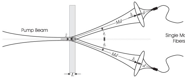
Figure 1: Schematic of collection setup.

The pump field transverse distribution is defined to be Gaussian with a waist of $\mathcal{W}_{\mathrm{p}}$, and we assume that the transverse crystal size is large relative to the pump beam, so we can take the cross section $S$ to be infinite. We also assume perfect transverse phase matching, i.e. $\bm{\kappa}_{\mathrm{p}}=\bm{\kappa}_{\mathrm{s}}+\bm{\kappa}_{\mathrm{i}}$. These assumptions allow the $\bm{\kappa}_{\mathrm{p}}$ and $\bm{\rho}$ integrals in Eq. (2) to be trivially performed

$$\int_{S}\textrm{d}^{2}\rho\left(\int\textrm{d}^{2}\kappa_{\mathrm{p}}~{}\widetilde{E}_{\mathrm{p}}(\bm{\kappa}_{\mathrm{p}})e^{i(\bm{\kappa}_{\mathrm{p}}\cdot\bm{\rho})}\right)e^{-i(\bm{\kappa}_{\mathrm{s}}+\bm{\kappa}_{\mathrm{i}})\cdot\bm{\rho}}~{}\propto~{}\widetilde{E}_{\mathrm{p}}(\bm{\kappa}_{\mathrm{i}}+\bm{\kappa}_{\mathrm{s}}).$$ (9)

We next assume that the longitudinal mismatch is small ($\Delta k_{z}L\ll 1$) and that we have near-perfect imaging ($c\epsilon d^{2}\kappa_{s,i}^{2}/(2\Omega_{s,i})\ll 1$). In this case, we can expand the exponentials in the Eq. (2) and use the result in Eq. (9) to obtain

$$A_{12}(\bm{\rho}_{1},\bm{\rho}_{2}) \propto ~{}\int\textrm{d}\omega\int\textrm{d}^{2}\kappa_{\mathrm{s}}\int\textrm{d}^{2}\kappa_{\mathrm{i}}\widetilde{E}_{\mathrm{p}}(\bm{\kappa}_{\mathrm{i}}+\bm{\kappa}_{\mathrm{s}})e^{iM(\bm{\kappa}_{\mathrm{s}}\cdot\bm{\rho}_{2}+\bm{\kappa}_{\mathrm{i}}\cdot\bm{\rho}_{1})}\tau_{1}(\omega)\tau_{2}(\omega)$$

$$\times~{}\left(1+\frac{i}{2}c\epsilon d^{2}\left(\frac{\kappa_{\mathrm{s}}^{2}}{\Omega_{\mathrm{s}}}+\frac{\kappa_{\mathrm{i}}^{2}}{\Omega_{\mathrm{i}}}\right)+\cdots\right)\left(1+\frac{i}{2}\Delta k_{z}L-\frac{1}{6}\left(\Delta k_{z}L\right)^{2}+\cdots\right)$$

The spectral filters defined by $\tau_{1}$ and $\tau_{2}$ are centered around the wavelengths $\Omega_{\mathrm{s}}$ and $\Omega_{\mathrm{i}}$ are both assumed to have a rectangular bandwidth $B$. We limit the expansions to first order and assume degenerate type-I phase-matching (i.e. $D=0$). The integrals yield

$$A_{12}(\bm{\rho}_{1},\bm{\rho}_{2})\propto BA^{o}_{12}(\bm{\rho}_{1},\bm{\rho}_{2})\left[1+\frac{iL}{2}\left(\alpha+\beta~{}a_{1}+\gamma~{}a_{2}-~{}\nu~{}a_{3}\right)\right]$$ (11)

where the zero order solution for the biphoton field is

$$A^{o}_{12}(\bm{\rho}_{1},\bm{\rho}_{2})\propto\frac{1}{M^{2}}E_{\mathrm{p}}\left(\frac{(\bm{\rho}_{1}+\bm{\rho}_{2})M}{2}\right)\delta(\bm{\rho}_{1}-\bm{\rho}_{2})\int\textrm{d}\omega\;\tau_{1}(\omega)\tau_{2}(\omega).$$ (12)

and the coefficients are

$$\alpha = \Delta k_{z}^{o}-D^{\prime}B^{2}/12$$ (13)

$$\beta = \frac{c}{2~{}n_{\mathrm{i}}(\Omega_{\mathrm{i}})\Omega_{\mathrm{i}}\cos\theta_{2}}+\frac{c\epsilon d^{2}}{\Omega_{\mathrm{i}}L}-\frac{c}{2~{}n_{\mathrm{p}}(\Omega_{\mathrm{p}},\theta_{\mathrm{p}})\Omega_{\mathrm{p}}}$$

$$\gamma = \frac{c}{2~{}n_{\mathrm{s}}(\Omega_{\mathrm{s}})\Omega_{\mathrm{s}}\cos\theta_{1}}+\frac{c\epsilon~{}d^{2}}{\Omega_{\mathrm{s}}L}-\frac{c}{2~{}n_{\mathrm{p}}(\Omega_{\mathrm{p}},\theta_{\mathrm{p}})\Omega_{\mathrm{p}}}$$

$$\nu = \frac{c}{2~{}n_{\mathrm{p}}(\Omega_{\mathrm{p}},\theta_{\mathrm{p}})\Omega_{\mathrm{p}}}$$

$$a_{1} = 4\frac{(1-M^{2}\rho_{1}^{2}/\mathcal{W}_{\mathrm{p}}^{2})}{\mathcal{W}_{\mathrm{p}}^{2}}$$

$$a_{2} = 4\frac{(1-M^{2}\rho_{2}^{2}/\mathcal{W}_{\mathrm{p}}^{2})}{\mathcal{W}_{\mathrm{p}}^{2}}$$

$$a_{3} = 2(\frac{2y_{2}\delta^{\prime}(y_{1}-y_{2})}{\mathcal{W}_{\mathrm{p}}^{2}}+\frac{\delta^{\prime\prime}(y_{1}-y_{2})}{M^{2}}),$$

With Eq. (11) in hand we are prepared to calculate the coupling of the biphoton field into the single mode fibers in our setup. To accomplish this we write $A_{12}$ as a coherent superposition of guided modes in the fiber as suggested in Ref. 16

$$A_{12}(\bm{\rho}_{1},\bm{\rho}_{2})=\sum_{l^{\prime}m^{\prime},lm}{A_{12}}^{l^{\prime}m^{\prime},lm}\varphi^{*}_{l^{\prime}m^{\prime}}(\bm{\rho}_{1})\varphi^{*}_{lm}(\bm{\rho}_{2})$$ (14)

The collection efficiency can then be calculated by

$$\eta_{12}=\frac{C_{12}}{\sqrt{C_{1}C_{2}}},$$ (15)

where $C_{12}$, $C_{1}$, and $C_{2}$ measure the square of the overlap between the biphoton field and the collection modes, and can be used to calculate singles and coincidence counting rates

$$C_{12} = \left|\int\textrm{d}^{2}\rho_{1}\int\textrm{d}^{2}\rho_{2}~{}A_{12}(\bm{\rho}_{1},\bm{\rho}_{2})\varphi^{*}_{l^{\prime}m^{\prime}}(\bm{\rho}_{1})\varphi^{*}_{lm}(\bm{\rho}_{2})\right|^{2}$$ (16)

$$C_{1} = \int\textrm{d}^{2}\rho_{2}\left|\int\textrm{d}^{2}\rho_{1}~{}A_{12}(\bm{\rho}_{1},\bm{\rho}_{2})\varphi^{*}_{l^{\prime}m^{\prime}}(\bm{\rho}_{1})\right|^{2}$$

$$C_{2} = \int\textrm{d}^{2}\rho_{1}\left|\int\textrm{d}^{2}\rho_{2}~{}A_{12}(\bm{\rho}_{1},\bm{\rho}_{2})\varphi^{*}_{lm}(\bm{\rho}_{2})\right|^{2}.$$

We assume the guided mode is a gaussian defined by

$$\varphi^{*}_{10}(\bm{\rho})=\sqrt{\frac{2}{\pi}}\frac{1}{\mathcal{W}_{f}}\exp\left[-\frac{\rho^{2}}{\mathcal{W}_{f}^{2}}\right]$$ (17)

where $\mathcal{W}_{f}$ is the width of the collection fiber. The waist of the collected mode imaged back to the crystal is given by $\mathcal{W}$, where $\mathcal{W}=M\mathcal{W}_{f}$. The collection efficiency is then obtained by using Eq.(11) and (15)

$$\eta_{12}\simeq\eta_{12}^{o}\frac{1+\frac{1}{4}L^{2}\chi_{1}^{2}}{1+\frac{1}{4}L^{2}\chi_{2}}$$ (18)

where the collection efficiency at the zero order of the perturbation theory (very thin crystals) is

$$\eta_{12}^{o}=4\frac{\mathcal{W}^{2}/\mathcal{W}_{\mathrm{p}}^{2}+1}{(\mathcal{W}^{2}/\mathcal{W}_{\mathrm{p}}^{2}+2)^{2}}$$ (19)

and the corrections are

$$\chi_{1} = \frac{\int\textrm{d}^{2}\rho_{2}\int\textrm{d}^{2}\rho_{1}~{}A_{12}^{o}(\bm{\rho}_{1},\bm{\rho}_{2})\varphi^{*}_{10}(\bm{\rho}_{1})\varphi^{*}_{10}(\bm{\rho}_{2})(\alpha+\beta a_{1}+\gamma a_{2}-\nu a_{3})}{\int\textrm{d}^{2}\rho_{2}\int\textrm{d}^{2}\rho_{1}A_{12}^{o}(\bm{\rho}_{1},\bm{\rho}_{2})\varphi^{*}_{10}(\bm{\rho}_{1})\varphi^{*}_{10}(\bm{\rho}_{2})}$$ (20)

$$\chi_{2} = \frac{\int\textrm{d}^{2}\rho_{2}\left|\int\textrm{d}^{2}\rho_{1}~{}A_{12}^{o}(\bm{\rho}_{1},\bm{\rho}_{2})\varphi^{*}_{10}(\bm{\rho}_{1})(\alpha+\beta a_{1}+\gamma a_{2}-\nu a_{3})\right|^{2}}{\int\textrm{d}^{2}\rho_{2}\left|\int\textrm{d}^{2}\rho_{1}A_{12}^{o}(\bm{\rho}_{1},\bm{\rho}_{2})\varphi^{*}_{10}(\bm{\rho}_{1})\right|^{2}}$$

We can perform these integrals using the expressions developed above to obtain

$$\chi_{1} = \alpha+\frac{2\nu}{\mathcal{W}^{2}}+\frac{8\beta-2\nu+8\gamma}{\mathcal{W}^{2}+2~{}\mathcal{W}_{\mathrm{p}}^{2}}$$ (21)

$$\chi_{2} = \alpha^{2}+\frac{12\nu^{2}}{\mathcal{W}^{4}}+\frac{16(\beta+\gamma)\nu}{\mathcal{W}^{2}\mathcal{W}_{\mathrm{p}}^{2}}+(\beta+\gamma)^{2}(\frac{1}{\mathcal{W}_{\mathrm{p}}^{4}}+\frac{1}{(\mathcal{W}^{2}+\mathcal{W}_{\mathrm{p}}^{2})^{2}})+4\alpha(\frac{\nu}{\mathcal{W}^{2}}+(\beta+\gamma)(\frac{1}{\mathcal{W}_{\mathrm{p}}^{2}}+\frac{1}{\mathcal{W}^{2}+\mathcal{W}_{\mathrm{p}}^{2}})).$$

3 Examples

To illustrate the use of Eq. (18) we consider a Lithium Iodate crystal with $L=2~{}\mathrm{mm}$. The crystal is pumped with 458 nm light with $\theta_{\mathrm{p}}=36^{\circ}$ and the collection modes are arranged to collect degenerate PDC emission at $\theta_{1}=\theta_{2}=1.5^{\circ}$ with a bandwidth of $B=2\times 10^{13}~{}\mathrm{s}^{-1}$ (about 10 nm). The magnification is fixed at $M=20$ and we assume that the collection mode waist occurs at the crystal with perfect imaging ($\epsilon=0$). Figure 2a plots the collection efficiency versus the pump waist for different collection mode waists. Figure 2b plots the term $\Delta k_{z}L$, and Figs. 2c and 2d plot the correction factors $\chi_{1}^{2}L^{2}/4$ and $\chi_{2}L^{2}/4$, respectively. Notice that the correction factors become significant for small pump waists (i.e. broad angular spectra of the pump).

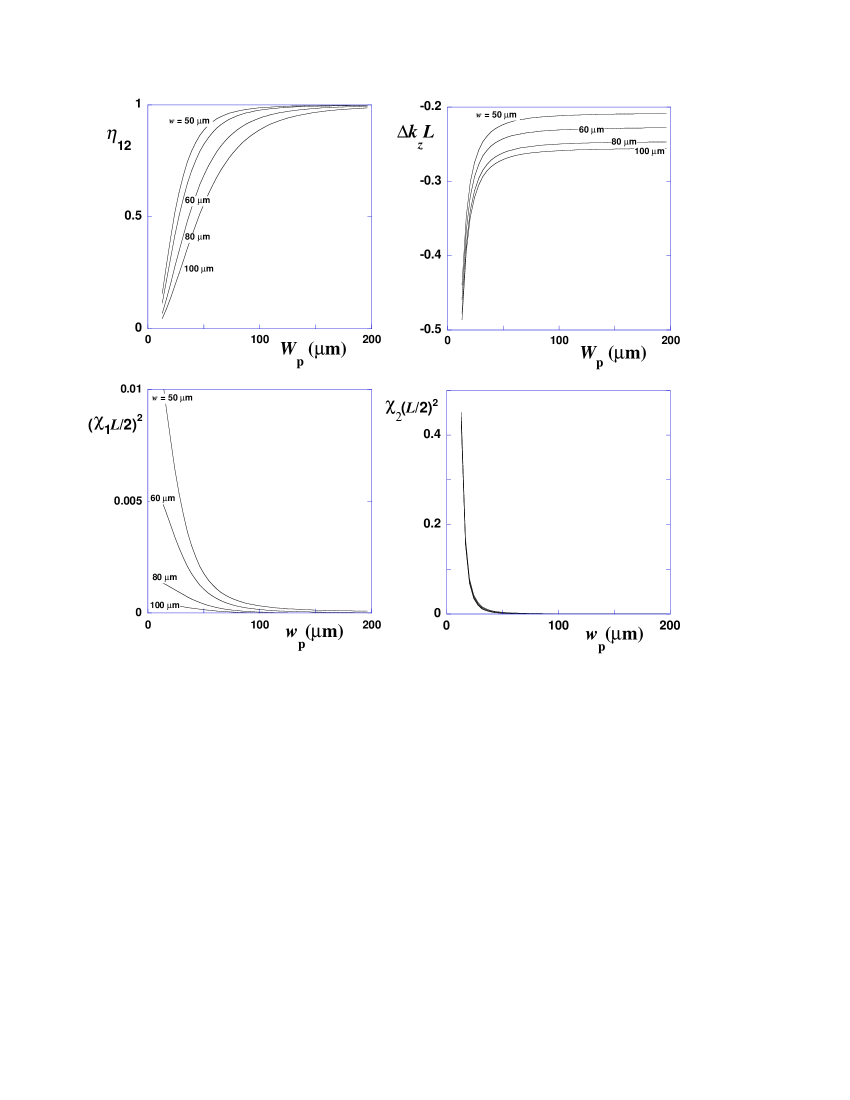
Figure 2: (a)Plot of the collection efficiency $\eta_{12}$ calculated versus the pump waist for various collection waists: $\mathcal{W}=50~{}\mu\mathrm{m}$, 60 $\mu$m, 70 $\mu$m, 80 $\mu$m, and 100 $\mu$m. The crystal length is $L=2~{}\mathrm{mm}$. (b) Plot of the longitudinal mismatch $\Delta k_{z}L$ in the same condition as case (a). (c) Plot of the correction factor $\chi_{1}^{2}L^{2}/4$. (d) Plot of $\chi_{2}L^{2}/4$ — the lines are so close that the individual collection mode waists are not labelled.

Figure 3 plots the collection efficiency versus the pump waist for four different crystal lengths: $L=0.1~{}\mathrm{mm}$, 2 mm, 3.5 mm and 4.5 mm, at various mode waists (all are in the valid range of the approximation). Note that for the case of $L=0.1~{}\mathrm{mm}$ (which satisfies the thin crystal approximation) the optimum collection efficiency can be obtained for all the collection modes by picking a sufficiently large pump waist. However for the longer crystals this is not the case. For example, if the collection mode is defined with $\mathcal{W}=20~{}\mu\mathrm{m}$ in the case of $L=4.5~{}\mathrm{mm}$ then the maximum collection efficiency that can be obtained is $\eta_{12}\approx 0.9$ regardless of how the pump waist is varied. However if we choose a collection mode with $\mathcal{W}=50~{}\mu\mathrm{m}$ the collection efficiency is $\eta_{12}\approx 1$ when $\mathcal{W}_{\mathrm{p}}>100~{}\mu\mathrm{m}$. (We limit the analysis here to crystal length of 4.5 mm because longer crystal push the validity of the approximations made earlier.) From Fig. 3 we conclude that we can take advantage of the higher signal levels from long crystals without sacrificing coupling efficiency provided that the pump waist and collection mode are scaled to appropriate values.

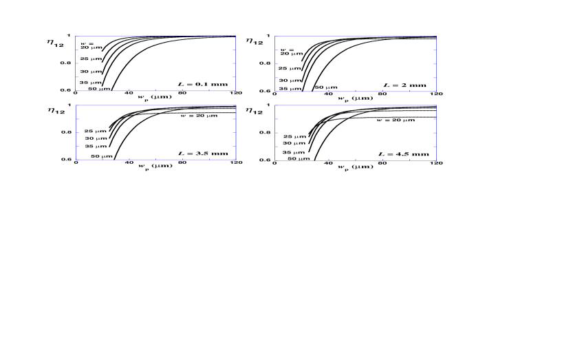
Figure 3: Plot of the collection efficiency $\eta_{12}$ calculated versus the pump waist for various crystal length from left to right $L=$0.1, $L$=2, $L$=3.5 and $L$=4.5 mm. Each graphics is evaluated for collection mode waists $\mathcal{W}=20~{}\mu\mathrm{m}$, 25 $\mu$m, 30 $\mu$m, 35 $\mu$m, 50 $\mu$m.

In Fig. 4a we plot the collection efficiency versus the crystal length for different magnifications (M=15, 20, 25, 30, 40) while maintaining a constant pump waist ($\mathcal{W}_{\mathrm{p}}=50~{}\mu\mathrm{m}$) and fiber size ($\mathcal{W}_{f}=1.5~{}\mu\mathrm{m}$). Figure 4b is the same as Fig. 4a but in the non-perfect imaging condition $\epsilon=0.4\mathrm{m}^{-1}$, which reduces the collection efficiency. Notice that as the crystal gets longer larger collection modes give a better coupling efficiency. Even though a longer crystal length reduces the collection efficiency obtainable for a given pump size, these longer crystals may still be desirable since they produce more overall signal. In addition, if the pump beam size is also be adjusted (as was done in the Fig. 2) it is still possible to get good coupling efficiency with a longer crystal.

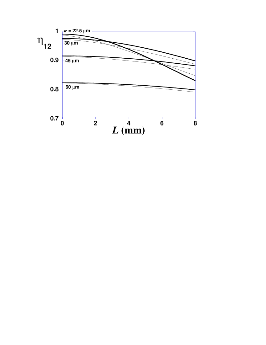
Figure 4: (a)Plot of the collection efficiency $\eta_{12}$ calculated versus the crystal length at $\mathcal{W}_{\mathrm{p}}$=50 $\mu$m for various collection mode waists. Heavy lines are calculated for perfect imaging ($\epsilon=0$) and narrow lines are calculated for the case of $\epsilon=0.4\mathrm{m}^{-1}$.

To verify that Eq. (18) is valid for the parameters that we have chosen, we must consider the numerical values of the corrections and verify that our approximation is in its range of validity. This is shown in Fig. 5 where the correction factors $\chi_{1}^{2}L^{2}/4$ and $\chi_{2}L^{2}/4$ are plotted versus the crystal length for different magnifications (M=15, 20, 25, 30, 40), maintaining the pump waist at $\mathcal{W}_{\mathrm{p}}=$50 $\mu$m and assuming the fiber core of $\mathcal{W}_{f}$=$1.5~{}\mu$m. It is clear that for the chosen parameters for crystals longer than about 8 mm the corrections become non-negligible.

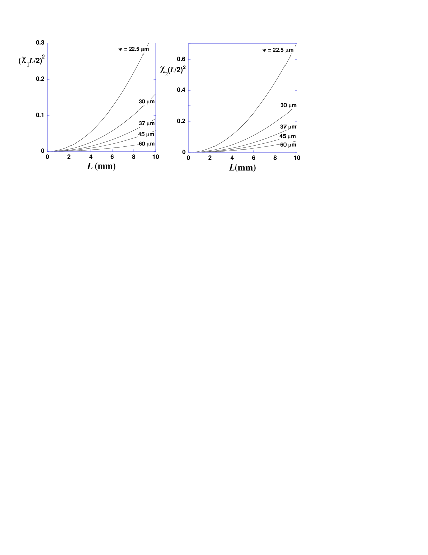
Figure 5: Plot of the correction factors $\chi_{1}^{2}L^{2}/4$ and $\chi_{2}L^{2}/4$ versus the crystal length for different collection mode waists, maintaining the pump waist at $\mathcal{W}_{\mathrm{p}}=$50 $\mu$m.

4 Conclusions

In the interest of optimizing the brightness of two-photon sources for use in emerging applications of quantum information, we have presented an analytical calculation of the collection efficiency of PDC light into single mode fibers. Our calculation was performed for the case of long pump pulse and type I PDC. These experimental conditions are similar to those used in many SPOD sources. We demonstrated that for crystals that are longer than those required by the thin crystal approximation (but still within the approximation made in the model) the maximum collection efficiency can be obtained at larger pump waists. However, as longer crystals are used the maximum achievable collection efficiency decreases. The approximations made in obtaining the expression for coupling efficiency limit the range of parameters that can be studied using this method. It is particularly important to pay close attention to the validity range of the approximations to assure meaningful results, as this has not been emphasized in some other works. Future work will move beyond the simple two-photon efficiency analysis to include an overall signal estimate that accounts for the effect of finite available pump on the total signal received. Experimental tests will be conducted to verify these analytical predictions.

This work was supported in part by DARPA/QUIST.

References

• [1] C. Bennett and G. Brassard, “Quantum cryptography: public key distribution and coin tossing,” in Proceedings of the IEEE International Conference on Computers, Systems and Signal Processing, p. 175, 1984.
• [2] C. Bennett and G. Brassard, “Quantum public key distribution system,” IBM Technical Disclosure Bulletin 28, p. 3153, 1985.
• [3] C. Bennett and G. Brassard, “The dawn of a new era for quantum cryptography: The experimental prototype is working!,” SIGACT NEWS 20, p. 78, 1989.
• [4] C. H. Bennett, F. Bessette, G. Brassard, L. Salvail, and J. Smolin, “Experimental quantum cryptography,” Lecture Notes in Computer Science 473, pp. 253–265, 1991.
• [5] A. Ekert, “Quantum cryptography based on Bell’s theorem,” Phys. Rev. Lett. 67, pp. 661–663, 1991.
• [6] C. Bennett, “Quantum cryptography using any two nonorthogonal states,” Phys. Rev. Lett. 68, pp. 3121–3124, 1992.
• [7] C. H. Bennett, G. Brassard, and N. D. Mermin, “Quantum cryptography without Bell theorem,” Phys. Rev. Lett. 68(5), pp. 557–559, 1992.
• [8] A. K. Ekert, J. G. Rarity, P. R. Tapster, and G. M. Palma, “Practical quantum cryptography based on 2-photon interferometry,” Phys. Rev. Lett. 69(9), pp. 1293–1295, 1992.
• [9] W. Tittel, J. Brendel, H. Zbinden, and N. Gisin, “Quantum cryptography using entangled photons in energy-time Bell states,” Phys. Rev. Lett. 84(20), pp. 4737–4740, 2000.
• [10] E. Knill, R. Laflamme, and G. J. Milburn, “A scheme for efficient quantum computation with linear optics,” Nature 409, pp. 46–52, 2001.
• [11] G. Brassard, N. Lutkenhaus, T. Mor, and B. C. Sanders, “Limitations on practical quantum cryptography,” Phys. Rev. Lett. 85(6), pp. 1330–1333, 2000.
• [12] T. B. Pittman, B. C. Jacobs, and J. D. Franson, “Single photons on pseudo-demand from stored parametric down-conversion,” Phys. Rev. A 66, pp. 042303 1–7, 2002.
• [13] A. Migdall, D. Branning, and S. Castelletto, “Tailoring single-photon and multiphoton probabilities of a single-photon on-demand source,” Phys. Rev. A 66, pp. 053805 1–4, 2002.
• [14] C. H. Monken, P. H. S. Ribeiro, and S. Padua, “Optimizing the photon pair collection effeciency: A step step towards a loophole-free Bell’s inequalities experiment,” Phys. Rev. A 57, pp. R2267–R2269, 1998.
• [15] C. Kurtsiefer, M. Oberparleiter, and H. Weinfurter, “High-efficiency entangled photon pair collection in type-ii parametric fluorescence,” Phys. Rev. A 6402(2), p. 023802, 2001.
• [16] F. A. Bovino, P. Varisco, A. M. Colla, G. Castagnoli, G. D. Giuseppe, and A. V. Sergienko, “Effective fiber coupling of entangled photons for quantum communication,” ArXiv:quant-ph/0303126 , 2003.
• [17] M. H. Rubin, “Transverse correlation in optical spontaneous parametric down-conversion,” Phys. Rev. A 54(6), pp. 5349–5360, 1996.