Iterative maximum-likelihood reconstruction in quantum homodyne tomography

Abstract

I propose an iterative expectation maximization algorithm for reconstructing the density matrix of an optical ensemble from a set of balanced homodyne measurements. The algorithm applies directly to the acquired data, bypassing the intermediate step of calculating marginal distributions. The advantages of the new method are made manifest by comparing it with the traditional inverse Radon transformation technique.

Quantum tomography is a technique of characterizing a state of a quantum system by subjecting it to a large number of quantum measurements, each time preparing the system anew. By varying the configuration of the measurement apparatus, one acquires the quantum statistics associated with different bases from which complete information about the state of the system can be extracted.

The ensemble’s density matrix can be evaluated from the experimental statistical data by a number of techniques. In this paper we are dealing with one such technique, the Maximum Likelihood (MaxLik) estimation. Assuming a particular density matrix $\hat{\rho}$, one can evaluate the likelihood (probability) of acquiring a particular set of measurement results. The ansatz of the MaxLik method is to find, among the variety of all possible density matrices, the one which maximizes the probability of obtaining the given experimental data set. To date, this method has been applied to various quantum and classical problems from quantum phase estimation [1] to reconstruction of entangled optical states [2, 3].

In the present work we discuss applications of likelihood maximization to quantum homodyne tomography - a method of characterizing a quantum state of an optical mode by means of multiple phase-sensitive measurements of its electric field’s quantum noise. Since its proposal [4] and first experimental implementation [5] in the early 1990s, quantum homodyne tomography has become a robust and versatile tool of quantum optics and has been applied in many different experimental settings. As any statistical method, it is compatible with the likelihood maximization approach. Yet so far experimentalists have used a clumsier and less accurate reconstruction algorithms based on the inverse Radon transformation. The goal of this paper is to provide an explicit numerical recipe for the MaxLik reconstruction of a quantum state from homodyne data and to demonstrate its advantages by applying it to bona fide experimental results.

The applications of MaxLik estimation to homodyne tomography have been investigated by Banaszek, who has reconstructed the photon-number distribution (the diagonal density matrix elements which correspond to a phase-randomized optical ensemble) from a Monte-Carlo simulated data set [6, 7]. In a subsequent publication [8], Banaszek et al. discussed the MaxLik estimation of the complete density matrix, but no explicit reconstruction algorithm has been presented.

The iterative scheme outlined here is based on that elaborated by Hradil et al. for discrete-variable states [2, 9, 10, 11] . Here we give its brief overview. Consider a large set of von Neumann measurements, each one projecting the state of the system onto an eigenstate of a measurement apparatus $\left|y_{j}\right\rangle$. The set of all possible outcomes $\{\left|y_{j}\right\rangle\}$ can be associated with either one or several measurement bases. Let $f_{j}$ be the frequency of occurrences for each outcome. Then, with the system being in the quantum state $\hat{\rho}$, the likelihood of a particular data set $\{f_{j}\}$ is

$$\mathcal{L}(\hat{\rho})=\prod_{j}{\rm pr}_{j}^{f_{j}},$$ (1)

where ${\rm pr}_{j}=\left\langle y_{j}\right|\hat{\rho}\left|y_{j}\right\rangle=\Tr[\hat{\Pi}_{j}\hat{\rho}]$ is the probability of the outcome $\left|y_{j}\right\rangle$ and $\hat{\Pi}_{j}=\left|y_{j}\right\rangle\left\langle y_{j}\right|$ denotes the projection operator.

To find the ensemble $\hat{\rho}$ which maximizes the likelihood (1), one introduces the operator

$$\hat{R}(\hat{\rho})=\sum_{j}\frac{f_{j}}{{\rm pr}_{j}}\hat{\Pi}_{j}$$ (2)

and notices that for the ensemble $\rho_{0}$ that is most likely to produce the observed data set, $f_{j}\propto{\rm pr}_{j}$. Furthermore, since the $\sum_{j}\hat{\Pi}_{j}\propto\hat{1}$, we find $\hat{R}(\hat{\rho}_{0})\propto\hat{1}$ and thus

$$\hat{R}(\hat{\rho}_{0})\hat{\rho}_{0}=\hat{\rho}_{0}\hat{R}(\hat{\rho}_{0})\propto\rho_{0}$$ (3)

as well as

$$\hat{R}(\hat{\rho}_{0})\hat{\rho}_{0}\hat{R}(\hat{\rho}_{0})\propto\rho_{0}.$$ (4)

The last relation forms the basis for the iterative algorithm. We choose some initial denstity matrix as, e.g., $\hat{\rho}^{(0)}=\mathcal{N}[\hat{1}]$, and apply repetitive iterations

$$\hat{\rho}^{(k+1)}=\mathcal{N}\left[\hat{R}(\hat{\rho}^{(k)})\hat{\rho}^{(k)}\hat{R}(\hat{\rho}^{(k)})\right],$$ (5)

where $\mathcal{N}$ denotes normalization to a unitary trace. Each step will monotonically increase the likelihood associated with the current density matrix estimate while the latter will asymptotically approach the maximum-likelihood ensemble $\hat{\rho}_{0}$. This iterative scheme can be viewed as a special case of the classical expectation-maximization algorithm [12].

Now we turn to the main subject of the paper and consider a homodyne tomography experiment performed on an optical mode prepared in some quantum state $\hat{\rho}$. In an experimental run one measures the field quadrature at various phases of the local oscillator. Each measurement is associated with the observable $\hat{X}_{\theta}=\hat{X}\cos\theta+\hat{P}\sin\theta$, where $\hat{X}$ and $\hat{P}$ are the canonical position and momentum operators and $\theta$ is the local oscillator phase.

For a given phase $\theta$, the probability to detect a particular quadrature value $x$ is proportional to

$${\rm pr}_{\theta}(x)={\rm Tr}[\hat{\Pi}(\theta,x)\hat{\rho}],$$ (6)

where $\hat{\Pi}(\theta,x)=\left|\theta,x\right\rangle\!\left\langle\theta,x\right|$ is the projector onto this quadrature eigenstate. In the Fock (photon number state) basis, the projection operator is expressed as

$$\Pi_{mn}(\theta,x)=\left\langle m\right|\hat{\Pi}(\theta,x)\left|n\right\rangle=\left\langle m|\theta,x\right\rangle\left\langle\theta,x|n\right\rangle,$$ (7)

where the overlap between the number and quadrature eigenstates is given by the well known stationary solution of the Schrödinger equation for a particle in a harmonic potential:

$$\left\langle n|\theta,x\right\rangle=e^{in\theta}\left(\frac{2}{\pi}\right)^{1/4}\frac{H_{n}(\sqrt{2}x)}{\sqrt{2^{n}n!}}\ \exp(-x^{2}),$$ (8)

with $H_{n}$ denoting the Hermite polynomials.

Because a homodyne measurement generates a continuous value, one cannot apply the iterative scheme (5) directly to the experimental data. One way to deal with this difficulty is to discretize the data by binning it up according to $\theta$ and $x$ and counting the number of events $f_{\theta,x}$ belonging to each bin. In this way, a number of histograms, which represent the marginal distributions of the desired ensemble’s Wigner function, can be constructed. They can then be used to implement the above reconstruction procedure.

However, discretization of continuous experimental data will inevitably lead to a loss of precision. To lower this loss, one needs to reduce the size of a single bin and increase the number of bins. In the limiting case of infinitely small bins, $f_{\theta,x}$ takes on the values of either 0 or 1, so the likelihood of a data set $\{(\theta_{i},x_{i})\}$ is given by

$$\ln\mathcal{L}=\sum_{i}\ln{\rm pr}_{\theta_{i}}(x_{i}),$$ (9)

and the iteration operator (2) becomes

$$\hat{R}(\hat{\rho})=\sum_{i}\frac{\hat{\Pi}(\theta_{i},x_{i})}{{\rm pr}_{\theta_{i}}(x_{i})},$$ (10)

where $i=1\dots N$ enumerates individual measurements. The iterative scheme (5) can now be applied to find the ensemble which maximizes the likelihood (9).

In practice, the iteration algorithm is executed with the density matrix in the photon number (Fock) representation. Since the Hilbert space of optical states is of infinite dimension, the implementation of the algorithm requires its truncation so the Fock terms above a certain threshold are excluded from the analysis. This assumption conforms to many practical experimental situations in which the intensities of fields involved are a priori limited.

It is instructive to compare the maximum likelihood quantum state estimation with the traditional methods employed in homodyne tomography: reconstruction of the Wigner function by means of the inverse Radon transformation [13] and evaluation of the density matrix using quantum state sampling [14, 15]. Fig. 1 shows application of these two techniques to the experimental data from Ref. [16]. The data set consists of 14152 quadrature samples of an ensemble approximating a coherent superposition of the single-photon and vacuum states.

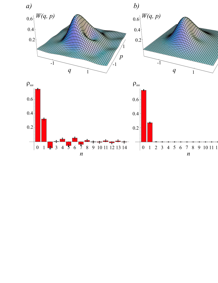
Figure 1: Estimation of an optical ensemble from a set of 14152 experimental homodyne measurements [16] by means of the inverse Radon transformation (a) and the likelihood maximization algorithm (b). The Wigner function and the diagonal elements of the reconstructed density matrix are shown. The inverse Radon transformation in (a) was performed by means of the filtered back-projection algorithm with the cutoff frequency of 6.3. The statistical uncertainties in (b) were determined by means of a Monte-Carlo simulation (see text).

The reconstruction shown in the figure reveals the advantages of the MaxLik technique in comparison with the standard algorithm. First, the finite amount and a discrete character of the data available leads necessarily to statistical noise which prevents one from extracting complete information about a quantum state of infinite dimension. To deal with this issue, both techniques apply certain assumptions on the ensemble to be reconstructed. While the MaxLik algorithm truncates the Fock space, the filtered back-projection imposes low pass filtering onto the Fourier image of the Wigner function, i.e. assumes the ensemble to possess a certain amount of “classicality” [17]. The latter assumption is dictated by mathematical convenience and is much less physically founded than the former. The ripples visible in the Wigner function reconstruction in Fig. 1(a) are a direct consequence of statistical noise and are associated with unphysical high number terms in the density matrix. Such ripples are typical of the inverse Radon transformation [18, 19].

Second, the back-projection algorithm does not impose any a priori restrictions on the reconstructed ensemble. This may lead to unphysical features in the latter, such as negative diagonal elements of the density matrix in Fig. 1(a). The MaxLik technique, on the other hand, allows to incorporate the positivity and unity-trace constraints into the reconstruction procedure, thus always yielding a physically plausible ensemble [6, 7].

A third important advantage of the MaxLik technique is the possibility to incorporate the detector inefficiences. In a practical experiment, the photodiodes in the homodyne detector are not 100% efficient, i.e. they do not transform every incident photon into a photoelectron. This leads to a distortion of the quadrature noise behavior which needs to be adjusted for in the reconstructed ensemble.

A common model for a homodyne detector of non-unitary efficiency $\eta$ is a perfect detector preceded by a fictitious beam splitter of transmission $\eta$. The reflected mode is lost so the incident density matrix undergoes, in transmission through the imaginary beam splitter, a so-called generalized Bernoulli transformation [13]:

$$\left\langle m\right|\hat{\rho}_{\eta}\left|n\right\rangle=\sum_{k=0}^{\infty}B_{m+k,m}(\eta)B_{n+k,n}(\eta)\left\langle m+k\right|\hat{\rho}_{0}\left|n+k\right\rangle,$$ (11)

where $\hat{\rho}_{0}$ and $\hat{\rho}_{\eta}$ are the density matrices of the original and transmitted ensembles, respectively, and $B_{n+k,n}=\sqrt{\left({n+k}\atop{n}\right)\eta^{n}(1-\eta)^{k}}$. Under these circumstances the probability (6) of detecting a quadrature value $x$ becomes

$${\rm pr}_{\theta}^{\eta}(x) = \left\langle\theta,x\right|\hat{\rho}_{\eta}\left|\theta,x\right\rangle$$

$$= \sum_{m,n=0}^{\infty}\sum_{k=0}^{\infty}B_{m+k,m}(\eta)B_{n+k,n}(\eta)\left\langle n|\theta,x\right\rangle\left\langle\theta,x|m\right\rangle\left\langle m+k\right|\hat{\rho}_{0}\left|n+k\right\rangle,$$

so the projection operator $\hat{\Pi}(\theta,x)$ becomes replaced by a POVM element given by

$$\hat{E}_{\eta}(\theta,x)=\sum_{m,n,k}B_{m+k,m}(\eta)B_{n+k,n}(\eta)\left\langle n|\theta,x\right\rangle\left\langle\theta,x|m\right\rangle\left|n+k\right\rangle\left\langle m+k\right|.$$ (13)

Aware of the homodyne detector efficiency $\eta$, one runs the iterative algorithm (5) and reconstructs the original density matrix $\hat{\rho}_{0}$ [8].

Theoretically, it is also possible to correct for the detector inefficiencies by applying the inverted Bernoulli transformation after an efficiency-uncorrected density matrix has been reconstructed [20]. However, this may give rise to unphysically large density matrix elements associated with high photon numbers. With the inefficiency correction incorporated, as described above, into the reconstruction procedure, such terms do not arise [7].

It is interesting to discuss the MaxLik reconsruction of the density matrix in comparison with the point-by-point reconstruction of the Wigner function as proposed in [21]. To determine the value of the Wigner function at a specific point $(p,q)$ in the phase space, Ref. [21] proposes to apply a phase-dependent shift to the experimental data which corresponds to a displacement of the point $(p,q)$ to the phase space origin. Then one reconstructs a phase-averaged ensemble according to Refs. [6, 7], and calculates the value of the Wigner function at the origin of the displaced phase space, which is equal to that at the desired location in the undisplaced phase space.

This scheme may appear more involved than the one proposed here, as one needs to run a separate iteration series for every point in which the Wigner function is to be calculated. However, due to a smaller number of parameters and a simplified iteration step, each iteration takes less time and the series converges faster. The choice of a particular scheme depends on a specific task and on the chosen truncation threshold in the Fock space. It is important to note that the scheme [21] does not impose any a priori restrictions onto the ensemble being reconstructed, and therefore the latter is not guaranteed to be physically meaningful.

Finally, we discuss statistical uncertainties of the reconstructed density matrix. In generic MaxLik algorithms, they are typically estimated as an inverse of the Fisher information matrix [22, 23] $G=\partial^{2}\mathcal{L}(\vec{t})/\partial\vec{t}\partial\vec{t}^{\prime}$, where $\vec{t}$ denotes a set of independent parameters with respect to which the likelihood is evaluated. Because the density matrix elements are not fully independent but bound by the positivity and unity trace constraints, one expresses the density matrix as a product $\hat{\rho}=\hat{T}^{\dagger}\hat{T}/\Tr[\hat{T}^{\dagger}\hat{T}]$. Now the constraints for $\hat{\rho}$ are satisfied for any random $\hat{T}$ and one can regard the elements of the latter as free parameters in evaluating the Fisher information [8, 24].

A sensible alternative is offered by a clumsy, yet simple and robust technique of simulating the quadrature data that would be associated with the estimated ensemble $\hat{\rho}_{ML}$ if it were the true state. One generates a large number of random sets of homodyne data according to Eq. (6), then applies the MaxLik reconstruction scheme to each set and obtains a series of density matrices $\hat{\rho}^{\prime}_{k}$ each of which approximates the original matrix $\hat{\rho}_{ML}$. The average difference $\langle|\hat{\rho}_{ML}-\hat{\rho}^{\prime}_{k}|\rangle_{k}$ evaluates the statistical uncertainty associated with the reconstructed density matrix.

References

References

- [1] Řeháček J, Hradil Z, Zawisky M, Pascazio S, Rauch H, and Peřina J 1999 Phys. Rev. A 60, 473
- [2] Řeháček J, Hradil Z, and Ježek M 2001 Phys. Rev. A 63, 040303
- [3] James D F V, Kwiat P G, Munro W J and White A G 2001 Phys. Rev. A 64, 052312
- [4] Vogel K and Risken H, 1989 Phys. Rev. A 40, 2847
- [5] Smithey D T, Beck M, Raymer M G, and Faridani A 1993 Phys. Rev. Lett. 70, 1244 ;
- [6] Banaszek K 1998 Phys. Rev. A 57, 5013
- [7] Banaszek K 1998 Acta Phys. Slov. 48, 185
- [8] Banaszek K, D’Ariano G M, Paris M G A, and Sacchi M F 2000 Phys Rev A 61, 010304
- [9] Hradil Z 1997 Phys. Rev. A 55, 1561
- [10] Hradil Z, Summhammer J, Rauch H 1999 Phys. Lett A 261 20
- [11] Fiurášek J 2001 Phys. Rev. A 64, 024102
- [12] Vardi Y and Lee D 1993 J. R. Statist. Soc B 55 569
- [13] Leonhardt U, 1997 Measuring the Quantum State of Light (Cambridge University Press)
- [14] D’Ariano G M, Leonhardt U, Paul H 1995 Phys. Rev. A 52, 1801
- [15] Leonhardt U, Raymer M G 1996 Phys. Rev. Lett. 76, 1985
- [16] Lvovsky A I and Mlynek J 2002 Phys. Rev. Lett 88 250401
- [17] Vogel W 2000 Phys. Rev. Lett. 84, 1849 (2000)
- [18] Breitenbach G, Schiller S, and Mlynek J 1997 Nature 387, 471 (1997)
- [19] Hansen H et al., 2001 Opt. Lett. 26, 1714
- [20] Kiss T, Herzog U, and Leonhardt U 1995 Phys. Rev. A 52, 2433
- [21] Banaszek K 1999 Phys. Rev. A 59 4797
- [22] Rao C R 1945 Bull. Calcutta Math. Soc. 37 81;
- [23] Cramér H 1946 Mathematical methods of statistics (Princeton University Press)
- [24] Usami K, Nambu Y, Tsuda Y, Matsumoto K and Nakamura K 2003 Phys. Rev. A 68 022314