Simultaneous Measurement of Non-commuting Observables
and Quantum Fractals on Complex Projective Spaces

Abstract

The simultaneous measurement of several noncommuting observables is modeled by using semigroups of completely positive maps on an algebra with a non-trivial center. The resulting piecewise-deterministic dynamics leads to chaos and to nonlinear iterated function systems (quantum fractals) on complex projective spaces.

I Introduction

From the very beginning quantum mechanics has been formulated in rather abstract mathematical terms: operators, commutators, eigenvalues, eigenvectors, etc. For the most part, the accompanying physical interpretations were discovered as surprises rather than due to any deeper understanding of what all this new theory was about. Much of the axiomatization of quantum theory originated in the works of John von Neumann, culminating in his classic monograph “Mathematical Foundations of Quantum Theory” Neu . But physics is not always as simple as mathematicians would like it to be. Even if the criteria of mathematical elegance and simplicity are often useful in sorting out candidates for possible formal descriptions of reality, Nature herself has proven to have a sense of elegance that quite often goes deeper than what we would naively expect. The unfortunate result of the lack of deeper understanding of the physical foundations of quantum theory (as exemplified by the famous discussions between Einstein and Bohr, with Einstein exclamating: “God does not play dice”, and Bohr responding: “Einstein, stop telling God what to do”) was that the theory has been axiomatized, including the concept of ‘measurement’. In this way for many many years only a few brave physicists dared to notice that the emperor has no clothes and say it aloud. As we have stressed elsewhere jad94c John Bell bell89 ; bell90 deplored the misleading use of the term ‘measurement’ in quantum theory. He opted for banning this word altogether from our quantum vocabulary, together with other vague terms such as ‘macroscopic’, ‘microscopic’, and ‘observable’. (Today he would probably add to his list two other terms of similarly dubious validity: ‘environment’, and ‘environmentally induced decoherence’.) He suggested that we ought to replace the term ‘measurement’ with that of ‘experiment’ bell87a , and also not to even speak of ‘observables’ (the things that seem to call for an ‘observer’) but to introduce, instead, the concept of ‘beables’ bell87b – the things that objectively ‘happen–to–be (or not–to–be)’, independent of whether there is some ‘observer’, even if only in the future wheeler83 , or not. In his scrupulous critical analysis of the quantum measurement problem bell90 , “Against Measurement,” John Bell indicates that to make sense of the usual mumbo jumbo one must assume either that (i) in addition to the wave function $\psi$ of a system one must also have variables describing the classical configuration of the apparatus or (ii) one must abrogate the Schrödinger evolution during measurement, replacing it by some sort of collapse dynamics.

The theory of quantum events (EQT), outlined in Section 2, combines (i) and (ii): there are additional classical variables, commonly referred to as ‘superselection rules’, and because of the coupling between these variables and the quantum degrees of freedom, the evolution is not exactly the unitary Schrödinger evolution, and it leads to collapses, in particular in measurement-like situations.

It is to be noted that Bell criticized both (i) and (ii), because both ascribe a special fundamental role to ‘measurement’, which seems implausible and makes vagueness unavoidable. EQT takes his valid criticism into account. In EQT we make a distinction between a measurement and an experiment. Both have a definite meaning within EQT. According to the general philosophy of EQT, our universe, one that we perceive and are trying to describe and understand, can be considered as being ‘an experiment’ – performed by Nature herself. This is in total agreement with Bell; it is also in agreement with the philosophy of John Wheeler, as outlined in wheeler83 ; wheeler89 . John A. Wheeler stressed repeatedly wheeler83 : “No elementary quantum phenomenon is a phenomenon until it is a registered (‘observed,’ ‘indelibly recorded’) phenomenon.” But, he did not give a definition of ‘being recorded’ (though he stressed that human ‘observers’ are neither primary nor even necessary means by which quantum potentials become ‘real’) – and we now understand why: Because such a definition could not have been given within the orthodox quantum theory. It is given in EQT – see Section $2$ below.

Historically, physicists arrived at the quantum formalism by a formal process known as ‘quantization’. Bohr’s quantization, Sommerfeld’s quantization, geometric quantization, deformation quantization … Today there is a multitude of formal quantization procedures, each leading to the end result that classical quantities are being formally replaced by linear operators that, in general, do not commute. The same components of position and momentum do not commute. Different components of spin do not commute. In each case the quantum commutation relations involve Planck’s constant on the right hand side. It is normally considered that it is not possible to measure simultaneously several noncommuting observables. One usually quotes in this respect the celebrated Heisenberg’s uncertainty relations. One must notice that, in his classic monograph Neu , John von Neumann was very careful in this respect, and he stressed explicitly that formal mathematical relations in no way indicate impossibility of a simultaneous and precise measurements of, say, position and momentum. He relied completely, in his account of the ‘physical interpretation’ of uncertainty relations, on the ‘thought experiments’ of Bohr and Heisenberg. Various textbook authors treat the subject in a different way. A reasonable and modern account of the problem is presented ingarden89 , where the authors present the standard derivation of Robertson’s inequality (2), and then add the following commentary:

“It follows from the Heisenberg’s uncertainty principle, and from the Theorem VII.1, that momentum and position are not commensurable, that is there is no generalized observable A such that

$$A(\Delta\times{\bf R}^{1}) =E^{Q}(\Delta),$$

$$A({\bf R}^{1}\times\Delta) =E^{P}(\Delta),$$

for $\Delta\subset{\cal B}({\bf R}^{1})$. However, that does not mean that quantum mechanics excludes the possibility of a simultaneous measurement of $P$ and $Q$. In experimental technique we are dealing with a simultaneous measurement of the momentum and position. For instance, we observe a particle in a Wilson chamber. From the observation of a particle track we determine its momentum and position. For a charged particle we deduce its momentum by placing the Wilson chamber in a magnetic field, and by measuring the curvature of the track. Even in a situation when we are only measuring the momentum of the particle, we have some knowledge of its position, for instance that the particle is within the volume of the measuring apparatus. The point is that in those situations we are not talking about the simultaneous measurement in the exact sense (description by spectral measures), but only about an approximate measurement, with a given uncertainty - such as a measurement described in example 6, section 12.1. The advantage of the formalism of generalized observables [i.e. using positive operators rather than idempotents ] is a possibility of a mathematical description of such a situation.”

In EQT indeed we are using positive operators and projections, but that is not important for the very modeling of the simultaneous measurement of non-commuting observables. In EQT fuzziness results in self-similarity and fractal patterns, but is not a necessary feature of the chaotic dynamics resulting from noncomeasurabilty. Masanao Ozawa, in a recent series of papers ozawa2001 ; ozawa2002 ; ozawa2003a ; ozawa2003b ; ozawa2003c , reviewed the actual status of theories of state reduction and joint measurement of non-commuting observables. Let us recall that for any pair of observables $A$ and $B$ we have the following relation Rob29 :

$$\Delta_{\rho}A\Delta_{\rho}B\geq\frac{1}{2}|\langle[A,B]\rangle_{\rho}|,$$ (2)

where $\langle\cdots\rangle_{\rho}$ stands for the mean value in the given state $\rho$, $\Delta_{\rho}A$ and $\Delta_{\rho}B$ are the standard deviations of $A$ and $B$, defined by $\Delta_{\rho}X=(\langle X^{2}\rangle_{\rho}-\langle X\rangle^{2}_{\rho})^{1/2}$ for $X=A,B$, and the square bracket stands for the commutator, i.e., $[A,B]=AB-BA$. In particular, for two conjugate observables $Q$ and $P$, which satisfy the canonical commutation relation

$$[Q,P]=i\hbar,$$ (3)

we obtain Kennard’s inequality Ken27

$$\Delta_{\rho}Q\Delta_{\rho}P\geq\frac{\hbar}{2}.$$ (4)

In ozawa2001 Ozawa concludes that

“… the prevailing Heisenberg’s lower bound for the noise-disturbance product is valid for measurements with independent intervention, but can be circumvented by a measurement with dependent intervention. An experimental confirmation of the violation of Heisenberg’s lower bound is proposed for a measurement of optical quadrature with currently available techniques in quantum optics.”

In a recent paper of this series ozawa2003b Ozawa writes

“Robertson’s and Kennard’s relations are naturally interpreted as the limitation of state preparations or the limitation of the ideal independent measurements on identically prepared systems Bal70 ; Per93 . Moreover, the standard deviation, a notion dependent on the state of the system but independent of the apparatus, cannot be identified with the imprecision of the apparatus such as the resolution power of the $\gamma$ ray microscope. Thus, it is still missing to correctly describe the unavoidable imprecisions inherent to joint measurements of noncommuting observables. ”

Although our criticism of the standard treatment of the measurement process and of the interpretation of the uncertainty relations goes much deeper, we do agree with the above conclusions.

I.1 Quantum Events Theory - Duality

EQT starts with the realization that any formal description of Reality must have a dual, partly classical and partly quantum nature. Those who deny this, contradict themselves by the very act of denying. Indeed, as stressed already by Niels Bohr, the sentences that they write, the conclusions they come to, are all classical in nature. In bell87a John Bell writes:

“But we cannot include the whole world in the wavy part. For the wave of the world is no more like the world we know than the extended wave of the single electron is like the tiny flash on the screen. We must always exclude part of the world from the wavy ‘system’, to be described in a ‘classical’ ‘particulate’ way, as involving definite events rather than just wavy possibilities.”

The fact of communicating anything through some channel, in finite time, is an ‘event’ – and as such, it is classical. It happens. However, there are no events in standard quantum theory, they do not belong to quantum dynamics, and the standard quantum theory does not provide us with any understanding of why, how, and when they happen. That is why the standard theory is incomplete. In 1986 John Bell, envisioning a possibility of creating a new, more complete theory wrote bell86 :

“And surely in fundamental theory this merging [of classical and quantum ] should be described not just by vague words but by precise mathematics? This mathematics would allow electrons to enjoy the cloudiness of waves, while allowing tables and chairs, and ourselves, and black marks on photographs, to be rather definitely in one place rather than another, and to be described in ‘classical’ terms. The necessary technical theoretical development involves introducing what is called ‘nonlinearity’, and perhaps what is called ‘stochasticity’, into the basic ‘Schrödinger equation’.”

EQT is a step in this direction, a step involving nonlinearity, non-unitarity, and stochasticity. The new mathematics of EQT, based on piecewise deterministic processes, enables us also to understand why the simultaneous measurement of noncommuting observables leads to chaotic dynamics that could not have been anticipated by the founders of quantum theory.

I.2 Central classical observables

In EQT we assume that, for one reason or another, the important object is a $\star$-algebra of operators $\mathfrak{A}.$ For historical reasons $\mathfrak{A}$ is called an ‘algebra of observables’, even if only normal operators, that is those which commute with their adjoints, are believed to be directly related to observable physical quantities. In EQT the elements of $\mathfrak{A},$ even if they can represent ‘physical quantities’, can neither be observed nor do they represent, as it is assumed within the standard interpretation ‘observational procedures’ – except in a limit that is rather unrealistic. We will see that operators in $\mathfrak{A}$ do exactly what they are supposed to do: they operate on states to produce new states that result from quantum events. They implement quantum jumps that accompany any event and any information gain related to the quantum system. It should be noted that in EQT we do not import any a priori probabilistic interpretation of the standard quantum theory. All interpretation is being derived from the Piecewise Deterministic Process (PDP) described below. Interpretation of eigenvectors, eigenvalues, mean values of observables, etc. should be derived from the dynamics of EQT. Part of the standard wisdom about eigenvalues and eigenvectors can, in fact, be justified within EQT, and so we will use it as a heuristic tool for constructing mathematical models of ‘real world’ situations. The algebra $\mathfrak{A}$ is usually assumed to be a $C^{\star}$ or a von Neumann algebra, but EQT can work also in spaces with indefinite scalar product or within a Clifford algebra framework. A generic algebra $\mathfrak{A}$ will have a nontrivial center ${\mathfrak{Z}}$ – the set of all $A\in{\mathfrak{A}}$ which commute with all the elements of ${\mathfrak{A}}.$ In particular ${\mathfrak{Z}}$ is Abelian – it represents the classical subsystem. Algebras with trivial center (i.e. center consisting of operators that are complex multiples of the identity) are called factors. Physicists insisting on the idea that there are no genuine classical degrees of freedom are, in fact, insisting on the idea that only factors should be used for an algebraic description of quantum systems. While it is true that every algebra can be decomposed, essentially uniquely, into a direct sum (or integral) of factors, restricting to factors alone is like restricting to prime numbers alone. While it is true that any integer can be decomposed into a product of prime numbers, insisting on the idea that only prime numbers should be used would be simply silly. Atoms build molecules. There would be no life without molecules. Similarly factors build more complex non-factors. According to our definition below, there would be no ‘events’ without non-factors! Thus there would be no data (recording a datum is an event) that could be used in experiments.

Each Abelian algebra has only one-dimensional irreducible representations. These are called characters, and the set of all characters of ${\mathfrak{Z}}$ is called the spectrum of ${\mathfrak{Z}}.$ By quite general representation theorems, each Abelian algebra is naturally isomorphic to an algebra of functions over its spectrum (continuous, measurable etc., depending on the type of the algebra). For simplicity we will assume that the spectrum of ${\mathfrak{Z}}$ is discrete – countable, or even finite. With proper care we could consider more general cases – as for instance in the SQUID-tank model, where the spectrum of ${\mathfrak{Z}}$ is a symplectic manifold - the phase space of a radio-frequency oscillator (cf. blaja93c ; olk97 , and also olk99 ; blaolk99a ; blaolk99b for other examples of working EQT models with a continuous spectrum of ${\mathfrak{Z}}$). Heuristically the points of the spectrum of ${\mathfrak{Z}}$ are the ‘pointer positions’ – that is, states of the classical subsystem – we will denote the spectrum of ${\mathfrak{Z}}$ by the letter ${\cal C}.$ Discrete changes of states of ${\cal C}$ are called events . When the set of classical states is discrete, then any change of it is discrete. But, for instance, in models with a continuous spectrum (as, for instance, when ${\cal C}$ is a phase space $\{q,p\}$) we will have a continuous evolution of the state of ${\cal C}$ that is interrupted by events, for instance jumps in the momentum $p$ (instantaneous boosts) in ${\cal C}.$

II An Outline of the formal scheme of Quantum Events Theory (EQT)

II.1 Completely Positive Maps

Historically, EQT started with an attempt at describing time evolution of a system with a non-trivial center, in the simplest case with ${\mathfrak{A}}={\mathfrak{A}}_{q}\otimes{\mathfrak{A}}_{cl},$ and ${\mathfrak{Z}}\approx{\mathfrak{A}}_{cl},$ where there would be a dynamical coupling and mutual exchange of information between the quantum and the classical degrees of freedom. Because algebra automorphisms preserve the center of any algebra, it was clear that automorphisms could not be used to this end. In a private communication with the author, Rudolph Haag, long ago, expressed his doubts as to the physical significance of the algebraic product in the algebra of observables. Even if the product $AB$ is useful in setting up the canonical commutation relations, the product of observables is not itself an observable and, therefore, need not be necessarily preserved by time evolution when irreversible recording is taking place. What seems to have physical meaning is positivity in the algebra, therefore the simplest generalization of the automorphic evolution takes us to semigroups of positive maps. Positivity itself is not a stable condition. Adding spurious degrees of freedom which do not participate in the dynamics can destroy positivity. The more stable condition is called ‘complete positivity’. It is defined as follows:

Let ${\mathfrak{A}},{\mathfrak{B}}$ be $C^{\star}$–algebras. A linear map $\phi:{\mathfrak{A}}\rightarrow{\mathfrak{B}}$ is Hermitian if $\phi(A^{\star})=\phi(A)^{\star}.$ It is positive iff $A\geq 0,$ $A\in{\mathfrak{A}}$ implies $\phi(A)\geq 0.$ Because Hermitian elements of a $C^{\star}$–algebra are differences of two positive ones – each positive map is automatically Hermitian. Let ${\mathfrak{M}}_{n}$ denote the $n$ by $n$ matrix algebra, and let ${\mathfrak{M}}_{n}({\mathfrak{A}})={\mathfrak{M}}_{n}\otimes{\mathfrak{A}}$ be the algebra of $n\times n$ matrices with entries from ${\mathfrak{A}}.$ Then ${\mathfrak{M}}_{n}({\mathfrak{A}})$ carries a natural structure of a $C^{\star}$–algebra. With respect to this structure a matrix ${\bf A}=(A_{ij})$ from ${\mathfrak{M}}_{n}({\mathfrak{A}})$ is positive iff it is a sum of matrices of the form $(A_{ij})=(A_{i}^{\star}A_{j}),\,$ $A_{i}\in{\mathfrak{A}}.$ If ${\mathfrak{A}}$ is an algebra of operators on a Hilbert space ${\mathfrak{H}}$, then ${\mathfrak{M}}_{n}({\mathfrak{A}})$ can be considered as acting on ${\mathfrak{H}}^{n}\doteq{\mathfrak{H}}\otimes{\mathbb{C}}^{n}=\oplus_{i=1}^{n}{\mathfrak{H}}.$ Positivity of ${\bf A}=(A_{ij})$ is then equivalent to $({\bf\Psi},{\bf A}{\bf\Psi})\geq 0\,,\,{\bf\Psi}\in{\mathfrak{H}}^{n},$ or equivalently, to $\sum_{i,j}(\Psi_{i},A_{ij}\Psi_{j})\geq 0$ for all $\Psi_{1},\ldots,\Psi_{n}\in{\mathfrak{H}}.$

A positive map $\phi$ is said to be completely positive or, briefly, CP iff $\phi\otimes id_{n}:{\mathfrak{A}}\otimes{\mathfrak{M}}_{n}\rightarrow{\mathfrak{B}}\otimes{\mathfrak{M}}_{n}$ defined by $(\phi\otimes id_{n})(A\otimes M)=\phi(A)\otimes M,\,M\in{\mathfrak{M}}_{n}$, is positive for all $n=2,3,\ldots.$ When written explicitly, complete positivity is equivalent to

$$\sum_{i,j=1}^{n}B_{i}^{\star}\phi(A_{i}^{\star}A_{j})B_{j}\geq 0$$ (5)

for every $A_{1},\ldots,A_{n}\in{\mathfrak{A}}$ and $B_{1},\ldots,B_{n}\in{\mathfrak{B}}.$ In particular every homomorphism of $C^{\star}$ algebras is completely positive. One can also show that if either ${\mathfrak{A}}$ or ${\mathfrak{B}}$ is Abelian, then positivity implies complete positivity. Another important example: if ${\mathfrak{A}}$ is a $C^{\star}$ algebra of operators on a Hilbert space ${\mathfrak{H}}$, and if $V\in{\mathfrak{B}}({\mathfrak{H}}),$ then $\phi(A)=VAV^{\star}$ is a CP map $\phi:{\mathfrak{A}}\rightarrow\phi({\mathfrak{A}}).$

In the quantum dynamics of open systems the unitary time evolution described by the Schrödinger equation is usually replaced by a semigroup of completely positive maps (also known as a ‘dynamical semigroup’) alicki87 ; alicki02 . Usually such semigroups are being studied on the von Neumann algebra ${\mathfrak{A}}$ of all bounded linear operators ${\mathfrak{A}}=L(\mathfrak{H})$ on a separable Hilbert space ${\mathfrak{H}}.$ In the algebraic framework emch we learn that more general von Neumann algebras can also appear in physical applications, in particular, as discussed above, algebras with a nontrivial center ${\mathfrak{Z}}=\mathfrak{A}\cap\mathfrak{A}^{\prime},$ where $\mathfrak{A}^{\prime}$ is the commutant of $\mathfrak{A}.$ The nontrivial central elements lead to superselection sectors (cf. landsman91 , and references therein), and, due to their commutativity with all observables, they represent the ‘classical observables’ of the theory. Applying open system dynamics to an algebra with a nontrivial center brings in new possibilities, with an interesting new result that there is a one-to-one correspondence between a class of completely positive semigroups and piecewise deterministic random processes (PDP – cf. davis93 ) on the space of pure states of the algebra. It has been shown that, in some cases, the associated piecewise deterministic process can be interpreted as a nonlinear iterated function system (IFS) on a complex projective space of rays in the Hilbert space ${\mathfrak{H}}$, with a fractal attractor, and with a range of Lyapunov’s exponents depending on a particular value of the coupling constant in the semigroup generator blajaol99a

In the present paper the algebra $\mathfrak{A}$ of observables will be assumed to be a von Neumann algebra. The points of the spectrum of its center ${\mathfrak{Z}}$ represent (pure) states of the Abelian subalgebra (superselection sectors). We will denote these states $\alpha=1,\ldots,m$. The algebra $\mathfrak{A}$ is then of the form $\mathfrak{A}=\oplus_{\alpha=1}^{m}\mathfrak{A}_{\alpha}$, where $\mathfrak{A}_{\alpha}$ are factors (that is they have a trivial center). We will be interested in the simplest case, where $\mathfrak{A}_{\alpha}=L({\mathfrak{H}}_{\alpha})$, where ${\mathfrak{H}}_{\alpha}$ is a Hilbert space of dimension (possibly infinite) $n_{\alpha}.$ Thus every element $A\in\mathfrak{A}$ is represented by a family $\{A_{\alpha}\}$ of operators $A_{\alpha}\in L({\mathfrak{H}}_{\alpha})$, or as a block diagonal matrix operator $A=diag(A_{1},\ldots,A_{m})$ on $\mathfrak{H}\doteq\oplus_{\alpha=1}^{m}{\mathfrak{H}}_{\alpha}.$ Every normal state $\rho$ of $\mathfrak{A}$ is represented by a density matrix on $\mathfrak{H}$ , that is by a family $\{\rho_{\alpha}\}$ of positive, trace-class operators on ${\mathfrak{H}}_{\alpha}$, with $\sum_{\alpha=1}^{m}Tr(\rho_{\alpha})=1,$ and $\rho(A)=\sum_{\alpha=1}^{m}Tr(\rho_{\alpha}A_{\alpha}).$

II.2 Dynamical Semigroups on an Algebra with a Center

The most general form of a generator of a completely positive semigroup is then given by the formula of Christensen and Evans chr , which generalizes the classical results of Gorini, Kossakowski and Sudarshan koss and of Lindblad lin to the case of an arbitrary $C^{\star}$–algebra. It is worthwhile to cite, after Lindblad, his original motivation:

The dynamics of a finite closed quantum system is conventionally represented by a one–parameter group of unitary transformations in Hilbert space. This formalism makes it difficult to describe irreversible processes like the decay of unstable particles, approach to thermodynamic equilibrium and measurement processes [$\ldots$]. It seems that the only possibility of introducing an irreversible behavior in a finite system is to avoid the unitary time development altogether by considering non–Hamiltonian systems.

Theorem 1 (Christensen – Evans)

Let $\alpha_{t}=\exp(Lt)$ be a norm–continuous semigroup of CP maps of a $C^{\star}$– algebra of operators ${\mathfrak{A}}\subset L({\mathfrak{H}}).$ Then there exists a CP map $\phi$ of ${\mathfrak{A}}$ into the ultraweak closure ${\bar{\mathfrak{A}}}$ and an operator $K\in{\bar{\mathfrak{A}}}$ such that the generator $L$ is of the form:

$$L(A)=\phi(A)+K^{\star}A+AK\,.$$ (6)

The set of all CP maps $\phi:\mathfrak{A}\rightarrow\mathfrak{A}$ is convex. Of particular interest to us are generators $L$ for which $\phi$ is extremal. Arveson arv , using the celebrated Stinespring theorem stinespring , proved that this is the case if and only if $\phi$ is of the form

$$\phi(A)=V^{\star}\pi(A)V\,,$$ (7)

where $\pi$ is an irreducible representation of ${\mathfrak{A}}$ on a Hilbert space ${\mathfrak{K}},$ and $V:{\cal H}\rightarrow{\mathfrak{K}}$ is a bounded operator (it must be, however, such that $V^{\star}\pi({\mathfrak{A}})V\subset{\mathfrak{A}}$). Then $\phi(I)=V^{\star}V.$ In the following we will assume that all $n_{\alpha}<\infty$, then ${\bar{{\mathfrak{A}}}}={\mathfrak{A}},$ so that $K=\{K_{\alpha}\}\in{\mathfrak{A}}.$ We will always assume that $\alpha_{t}(I)=I$ or, equivalently, that $L(I)=0.$ It is convenient to introduce $H_{\alpha}=i(K_{\alpha}-K_{\alpha}^{\star})/2\in L({\mathfrak{H}}_{\alpha}),$ then from $L(I)=0$ we get $K_{\alpha}+K_{\alpha}^{\star}=-\phi(I)_{\alpha},$ and so $K_{\alpha}=-iH_{\alpha}-\phi(1)_{\alpha}/2.$ Therefore we have

$$L(A)_{\alpha}=i\left[H_{\alpha},A_{\alpha}\right]+\phi(A)_{\alpha}-\{\phi(1)_{\alpha},A_{\alpha}\}/2,$$ (8)

where $\{\,,\,\}$ denotes the anticommutator. Using the Arveson result it is easy to see that, in our case, $\phi$ is a non-zero extremal CP map if and only if $V$ is if of the form $V=\{V_{\alpha\beta}\}$, where only one matrix entry $V_{\alpha_{0}\beta_{0}}:\mathfrak{H}_{\beta_{0}}\rightarrow\mathfrak{H}_{\alpha_{0}}$ is non-zero. Taking for $\phi$ a sum of maps of such a type we end up with a generator $L$ of the form:

$$L(A)_{\alpha}=i[H_{\alpha},A_{\alpha}]+\sum_{\beta}g_{\beta\alpha}^{\star}A_{\beta}\ g_{\beta\alpha}-\frac{1}{2}\{\Lambda_{\alpha},A_{\alpha}\},$$ (9)

where $g_{\alpha\beta}\in L({\mathfrak{H}}_{\beta},{\mathfrak{H}}_{\alpha})$ and

$$\Lambda_{\alpha}=\sum_{\beta}g_{\beta\alpha}^{\star}g_{\beta\alpha}\in L({\mathfrak{H}}_{\alpha}).$$ (10)

II.3 The Liouville Equation for States

Taking into account the duality between observables and states, given by the valuation $<\rho,A>=Tr(\rho A)=\sum_{\alpha=1}^{m}Tr(\rho_{\alpha}A_{\alpha}),$ the evolution equation for the semigroup ${\dot{A}}=L(A)$ can be rewritten in terms of states:

$${\dot{\rho}}_{\alpha}=-i[H_{\alpha},\rho_{\alpha}]+\sum_{\beta}g_{\alpha\beta}\rho_{\beta}g_{\alpha\beta}^{\star}-\frac{1}{2}\{\Lambda_{\alpha},\rho_{\alpha}\}.$$ (11)

Notice that the total trace is automatically conserved:

$$\frac{d}{dt}Tr(\rho)=\sum_{\alpha}Tr({\dot{\rho}}_{\alpha})=0.$$

In problems that are explicitly time-dependent, as it is in most cases where there is an explicit intervention of the ‘experimenter’, who sets up the characteristics of the measuring device according to the needs of the experiment, the maps $\phi$ and $K$, and thus the operators $H_{\alpha}$ and $g_{\alpha\beta}$ will depend on time, and they will generate a family $\alpha_{t}$ of CP maps, which will not have the semigroup property.

II.4 Ensemble and Individual Descriptions

There are two descriptions in EQT: the ensemble description and the individual description. The ensemble description is a deterministic, smooth Liouville evolution of statistical states. The individual description is piecewise deterministic process on the space of pure states, where a continuous, nonunitary, evolution is interrupted by discontinuous catastrophic events. One goes from the individual to the ensemble description by averaging over many sample paths. The averaging process smoothes out discontinuouities and nonlinearities.

The jump probabilities in the process will be computed from the formula:

$$p_{\alpha\rightarrow\beta}(\psi,t)=\|g_{\beta\alpha}(t)\psi\|^{2}/<\psi,\Lambda_{\alpha}(t)\psi>.$$ (12)

It has been shown in jakol95 that when the diagonal terms $g_{\alpha\alpha}$ all vanish, then there is a one-to-one correspondence between the solutions of the Liouville equation (11), and PDP processes on the space of pure states of the algebra $\mathfrak{A}$, where the process realizing the solution of Eq. (11) with the initial pure state $\rho=(0,\ldots,|\psi_{\alpha_{0}}><\psi_{\alpha_{0}}|,\ldots,0)$ is described as follows:
PDP Process: Given on input $t_{0},\alpha_{0},$ and $\psi_{0}\in{\mathfrak{H}}_{\alpha_{0}}$, with $\|\psi_{0}\|=1$, it produces on output $t_{1},\alpha_{1}$ and $\psi_{1}\in{\cal H}_{\alpha_{1}}$, with $\|\psi_{1}\|=1$. $1$) Choose uniform random number $r\in[0,1]$.
$2$) Propagate $\psi_{0}$ in ${\mathfrak{H}}_{\alpha_{0}}$ forward in time by solving:

$${\dot{\psi}}(t)=\left(-iH_{\alpha_{0}}(t)-\frac{1}{2}\Lambda_{\alpha_{0}}(t)\right){\psi}(t)$$ (13)

with initial condition $\psi(t_{0})=\psi_{0}$ until $t=t_{1}$, where $t_{1}$ is defined by

$$\|\psi(t_{1})\|^{2}=r.$$ (14)

$3$) Choose a uniform random number $r^{\prime}\in[0,1].$
$4$) Run through the classical states $\alpha=1,2,\ldots,m$ until you reach $\alpha=\alpha_{1}$ for which

$$\sum_{\alpha=1}^{\alpha_{1}}p_{\alpha_{0}\rightarrow\alpha}(\psi(t_{1}),t_{1})\geq r^{\prime}.$$ (15)

$5$) Set $\psi_{1}=g_{\alpha_{1}\alpha_{0}}(t_{1})\psi(t_{1})/\|g_{\alpha_{1}\alpha_{0}}(t_{1})\psi(t_{1})\|$.
Time evolution of an individual system is described by repeated application of the above algorithm, using its output as the input for each next step. If we want to study time evolution in a given interval $[t_{in},t_{fin}]$, then we apply the algorithm by starting with $t_{0}=t_{in}$, repeating it until we reach $t=t_{fin}$ somewhere in the middle of the propagation in step 2). Then we normalize the resulting state.

According to the theory developed in Ref. davis93 the jump process is an inhomogeneous Poisson process with intensity function $\lambda_{\alpha}(t)=\left(\psi(t),\Lambda_{\alpha}(t)\psi(t)\right)$. One way to simulate such a process is to move forward in time by small time intervals $\Delta t$, and make independent decisions for jumping with probability $\lambda_{\alpha}(t)\Delta t$. This leads to the probability $p$ of a jump to occur in the time interval $(t_{0},t)$ given by

$$p=1-\exp(-\int_{t_{0}}^{t}\lambda_{\alpha}(s)ds).$$ (16)

By using the identity $\log f(t)-\log f(t_{0})=\int_{t_{0}}^{t}{\dot{f}(s)}/f(s)\;ds,$ with $f(s)\doteq||\psi_{\alpha}(t)||^{2},$ it is easy to see that $p=1-\|\psi_{\alpha}(t)\|^{2}$ – which simplifies simulation – as we did in the step 2) above. This observation throws also some new light upon those approaches to the quantum mechanical description of particle decays that were based on non-unitary evolution.

By repeating the above event generating algorithm many times, always starting with the same state at the same initial time $t_{0}$, and ending it at the same final time $t,$ we will arrive at different final states with different probabilities. Let $\alpha_{0},\psi_{\alpha_{0}},t_{0}$ be the initial state, and let $\mu(\alpha_{0},\psi_{\alpha_{0}},t_{0};\alpha,\psi_{\alpha},t)$ be the probability density of arriving at the state $(\alpha,\psi_{\alpha})$ at time $t$. We may associate with this probability distribution a family of density matrices:

$$\rho_{\alpha}(t)=\int\mu(\alpha_{0},\psi_{\alpha_{0}},t_{0};\alpha,\psi_{\alpha},t)|\psi_{\alpha}><\psi_{\alpha}|d\psi_{\alpha},$$ (17)

so that $\sum_{\alpha}{\mbox{T}r}\rho_{\alpha}(t)=1$. This association is many to one. We lose in this way information. Nevertheless, as shown in jakol95 , the following theorem holds:

Theorem 2

The family $\rho_{\alpha}(t)$ satisfies the Liouville linear differential equation (11). Conversely, the PDP process with values in the pure states $\alpha,\psi_{\alpha}$ described above is the unique one leading to (11).

The Liouville equation (11) describes the time evolution of the statistical states of the total system. This is the standard, linear, master equation of statistical quantum physics, an equation that describes infinite statistical ensembles, not individual systems. Although the theorem quoted above tells us that the event generating algorithm follows essentially uniquely from the Liouville equation, we believe that it is the PDP process rather than the statistical description that will lead to future generalizations and extensions of the applicability of the quantum theory. For instance, in the above formalism it is assumed that the operators $g_{\alpha\beta}$ are linear. But they do not have to be. The operators $g_{\alpha\beta}$ represent couplings between the quantum system and a classical ‘detector pointer’, and jumps represents ‘events’ i.e. changes of the pointer state. The formalism has been, in particular, applied to the calculation of arrival times blaja95f and tunneling times for quantum particles tunneling through a potential barrier palao ; muga , to the calculation of relativistic time of arrival rus02a ; rus02b , and also for studying classical interventions in quantum systems peres00b .

II.5 Simple Examples

Physicists have long experience with constructing Hamiltonians ${H_{\alpha}}$ describing the action of external force fields and different known interactions between particles. But how do we construct the transition operators $g_{\alpha\beta}$? As has been noticed by many authors, any ‘measurement’ can be, in principle, reduced to a position measurement. Once we know how to measure the ‘pointer position’, it is argued, it is enough to set up an interaction between the apparatus and the system, both considered as quantum systems, and, when the measurement is ‘done’, read the pointer position. While we do not think that life is that simple, there is certainly some truth in the above, and therefore let us start with a simple model of position measurement. The position variable can be analyzed in terms of yes-no observations as to whether a given region of space is occupied or not. Thus our first example will describe a simple particle detector. In the next section we will describe how a simultaneous monitoring of several non-commuting observables can be modeled within EQT.

II.5.1 A single detector

A detector is a two-state device. It is often assumed that a detector destroys the particle, but, as a typical track in a cloud chamber shows, this need not be the case. There are several ways of building a model of a detector, and we will describe the simplest one, although not quite realistic. We would like to think of a detector as a two-state device, with two meta-stable states, denoted $0$ and $1$, able to jump from one state to another when detecting a signal. We will assume zero relaxation time, so that after detecting a signal, the detector is instantly ready to detect another signal. Heuristically a particle passing close to the detector can trigger its ‘flip’ from $0$ to $1$, or from $1$ to $0.$ We will be interested only in the simplest case, when the detection capability depends only on the particle location, and not on its energy or other characteristics.

Let us now specialize and consider a detector of particle presence at a location $a$ in space (of $n$ dimensions). Our detector has a certain range of detection and a certain efficiency. In a simple model we encode these detector characteristics in a gaussian function:

$$g(x)=\kappa^{1/2}\left(\frac{1}{\sigma\sqrt{\pi}}\right)^{n/2}\exp(-x^{2}/2\sigma^{2}),$$ (18)

where $\kappa$ is the detector sensitivity constant, $\sigma$ is a width parameter, and $n$ stands for the number of space dimensions.
If the detector is moving in space along some trajectory $a(t)$, and if the detector characteristics are constant in time and space, then we put: $g_{t}(x)=g(x-a(t))$. Let us suppose that the detector is in one of its states at $t=t_{0}$ and that the particle wave function is $\psi_{0}(x)$. Then, according to the algorithm described in section II.4, the probability $p$ of detection in the infinitesimal time interval $(t_{0},t_{0}+\Delta t)$ is given by $p\approx\int g_{t_{0}}^{2}(x)|\psi_{0}(x)|^{2}dx\cdot\Delta t$. In the limit $\sigma\rightarrow 0$, when $g^{2}_{t}(x)\rightarrow\kappa\,\delta(x-a(t))$ we get $p\approx\kappa|\psi_{0}(a(t_{0}))|^{2}\cdot\Delta t$. Thus, when $\Delta t<<1/\kappa,$ we approximately recover the usual Born interpretation, with the evident and necessary correction that the probability of detection is proportional to the length of exposure time of the detector.

III Measurement of noncommuting observables

EQT enhances the predictive power of the standard quantum theory, and it does it in a rather simple way. Once enhanced it predicts new facts and straightens old mysteries. The model that we have outlined above has several important advantages. One such advantage is of a practical nature: for example in blaja93c it is shown how to generate pointer readings in a tank radio–circuit coupled to a SQUID. In jad94b ; jad94c the algorithm generating detection events of an arbitrary geometrical configuration of particle position detectors, as for instance in a Wilson chamber, has been derived. As a particular case, in a continuous homogeneous limit we reproduced GRW spontaneous localization model (cf jad94c and references therein). Many other examples come from quantum optics, since the Quantum Monte Carlo model used there is a special case of our approach, namely when events are not fed–back into the system and thus do not really matter.

Another advantage of EQT is of a conceptual nature: in EQT we need only one postulate: that events can be observed . All the rest can and should be derived from this postulate. All probabilistic interpretation, everything that we have learned, or postulated, about eigenvalues, eigenvectors, transition probabilities, etc. can be derived from the formalism of EQT. Thus in blaja93a we have shown that the probability distribution of the eigenvalues of Hermitian observables can be derived from the simplest, measurement-like, coupling. Moreover, in jad94a it was shown that EQT can also give definite predictions for non–standard measurements, which are of particular interest here, namely those involving noncommuting observables, and that is so because in our scheme the contributions $g_{\alpha\beta}$ from different, non-commuting, devices add rather than multiply. In this respect, because the measurement process is dynamical in our approach, it is like adding non-commuting terms in a Hamiltonian – nobody has difficulty with adding a position function $A_{\mu}(x)$ to the momentum $p_{\mu}$ in a Hamiltonian. They act simultaneously and they act together.

Before we describe the model, and the resulting chaotic behavior and strange attractor on the quantum state space, let us first discuss in more detail the very question of the simultaneous measurability of non-commuting observables. As we mentioned in the Introduction, this subject has become quite controversial since the early formulation of Heisenberg’s uncertainty relations. Mathematically these relations are precise and leave no doubt about their validity, but the question of how to interpret them physically and philosophically has become a subject of hot discussions. Various views have been expressed on this subject. Clearly there are different opinions. For instance one of the early reviewers of the present paper wrote: “QM, is a complete theory, with precise, definite operational meanings attached to the terms ‘measurement’, ‘observable’ & c. Within its rules, the simultaneous measurement of non-commuting observables is impossible. This is well known and explained in any serious textbook, which the author should be referred to.” This sentence evidently contradicts the other sentence, from the textbook by Ingarden and Grabowski where, as already quoted in the Introduction, the authors write: “(…) However, that does not mean that quantum mechanics excludes the possibility of a simultaneous measurement of $P$ and $Q$. In experimental technique we are dealing with a simultaneous measurement of the momentum and position.” It seems that the reviewer does not distinguish state preparation procedure from measurements. To quote from Popper’s ‘Unended Quest’ popper :

“The Heisenberg formula do not refer to measurements; which implies that the whole current ‘quantum theory of measurement’ is packed with misinterpretations. Measurements which according to the usual interpretation of the Heisenberg formula are ‘forbidden’ are according to my results not only allowed, but actually required for testing these very formula.”

Hilary Putnam came to a similar conclusion putnam81 :

“Recently I have observed that it follows from just the quantum mechanical criterion for measurement itself that the ‘minority view’ is right to at least the following extent: simultaneous measurements of incompatible observables can be made . That such measurement cannot have ‘predictive value’ is true …”

These words, written more than twenty years ago, suggested that one should expect a chaotic behavior, and that this chaos and its characteristics ought to be studied, both theoretically and experimentally. Yet, for some reason, either no one noticed, or no one got interested in looking into the problem quantitatively. Of course the main theoretical obstacle was the unsolved quantum-mechanical measurement problem. A good , critical, discussion of current issues involved here, can be found in landsman94 . In the abstract of his paper Landsman states:

“We attempt to clarify the main conceptual issues in approaches to ‘objectification’ or ‘measurement’ in quantum mechanics which are based on superselection rules. Such approaches venture to derive the emergence of classical ‘reality’ relative to a class of observers; those believing that the classical world exists intrinsically and absolutely are advised against reading this paper.”

Even if Landsman is guilty of using the undefined, magical, word ‘environment’, as, for instance, in

“The prototype approach (Hepp) where superselection sectors are assumed in the state space of the apparatus is shown to be untenable. Instead, one should couple system and apparatus to an environment, and postulate superselection rules for the latter,”

he does a pretty good job in taking apart different approaches and in analyzing their weaknesses.

III.1 The simplest toy model - space and momentum are each only two-points.

In this example we will describe the simplest possible toy model of a simultaneous measurement of several non-commuting observables. The most celebrated example is, of course, the canonical pair of position and momentum observables. Although in principle easy, technically it is difficult to simulate on a computer, because the Hilbert space is infinite-dimensional. It is also somewhat difficult to analyze analytically, due to its continuous spectra. We will therefore choose here the maximally simplified model - technically easy, almost trivial, and yet demonstrating the whole idea.

The simplest, nontrivial ‘space’ has just two points, we will denote them ‘-1’ and ‘1’. The ‘translation group’ which operates on these two points has two elements: the identity element and the ‘flip’ that exchanges these two points. We realize this simple imprimitivity system in a two-dimensional Hilbert space ${\mathfrak{H}}={\mathbb{C}}^{2}.$ With the standard Pauli matrices $\sigma_{1},\,\sigma_{2},\,\sigma_{3}$ defined by

$$\sigma_{1}\>=\>\left(\begin{array}[]{cc}0&1\\ 1&0\end{array}\right)\quad\sigma_{2}\>=\>\left(\begin{array}[]{cc}0&-i\\ i&0\end{array}\right)\quad\sigma_{3}\>=\>\left(\begin{array}[]{cc}1&0\\ 0&-1\end{array}\right)$$

we represent the ‘position operator’ by $\sigma_{3}$, and the ‘momentum operator’ by $\sigma_{1}.$ Note that in our case $\sigma_{1}$ represents the unitary ‘flip’, while $(I+\sigma_{1})/2$ represents the ‘momentum’. We will need four detectors, two for detecting the position eigenvalues $q=-1$ and $q=+1$, and two for detecting the momentum eigenvalues $p=0$ and $p=+1.$ As, formally, this is a particular case of a more general situation, when we model a monitoring of several non-commuting spin projections, in what follows we will discuss this more general situation. As with the simple choice above, with four detectors, we will consider a simple, highly symmetric geometric pattern, so that the fractal and self-similarity effect are easily recognizable. Our quantum system will be therefore a single spin $1/2,$ with no spatial degrees of freedom. In order to construct a model within the framework of EQT we need to specify the classical system, its states, and the operations implementing transitions between the states. We will have a family of $n$ detectors, each of them can be excited independently of the others, so that the probability of two detectors being excited at the same time is zero. Therefore a state of the classical system will be a sequence of $n$ numbers, each number being $0$ or $1.$ There are $2^{n}$ of such states, and a possible change of state consists of adding $1\,\mbox{mod}\,2$ at $i$-th place. For instance, if we have three detectors, a possible transition between states can be $\alpha=(1,0,1)\longrightarrow\beta=(0,0,1)$ - a flip of the first detector. Only one detector can flip at a time. As for the spin system, we will identify the Hilbert spaces ${\mathfrak{H}}_{\alpha}\equiv{\mathfrak{H}}\equiv{{\mathbb{C}}}^{2},\;\alpha=1,\ldots,2^{n},$ corresponding to different states of the classical subsystems. In this way the total algebra $\mathfrak{A}$ will be represented as a tensor product $\mathfrak{A}=\mathfrak{A}_{q}\otimes\mathfrak{A}_{c}$ of its quantum and classical parts. Because the quantum system is a two-state system, so the quantum algebra $\mathfrak{A}_{q}=L({\mathfrak{H}})$ can be identified with the algebra of $2\times 2$ complex matrices. Pure states of the spin system are uniquely represented by points of the complex projective space ${\bf P}_{1}({{\mathbb{C}}})$, which is isomorphic to the sphere ${\bf S}^{2}$ or, equivalently, by one-dimensional projections of the form $\frac{1}{2}(I\>+\>\vec{n}\cdot\vec{\sigma}),$ where $\vec{n}$ is a unit vector in ${\mathbb{R}}^{3}$ - pointing in the direction of the spin.

To be specific, let us consider a simple and symmetric configuration of detectors, when the measuring apparatus consists of six yes-no polarizers corresponding to $n=6$ spin directions $\vec{n}_{i}$, $i=\,1,...,n$, arranged at the vertices of a regular octahedron along the directions $\vec{n}_{i},\>i=1,\ldots,n$:

$$\{\{\{0,0,1\},\{1,0,0\},\{0,1,0\},\\ \{-1,0,0\},\{0,-1,0\},\{0,0,-1\}\}.$$

Notice that the six vectors sum up to zero

$$\sum_{i=1}^{n}\vec{n}_{i}={\bf 0}.$$ (19)

We may assume that our spin evolves according to the Hamiltonian $H\,=\,\frac{\omega}{2}\sigma_{3}$, $\omega\geq 0.$ The coupling between the spin system and the detectors is specified by choosing six operators $a_{i},$ which correspond to the six vectors $\vec{n}_{i}$

$$a_{i}\;=\;\frac{1}{2}\,(I\>+\>\epsilon\,\vec{n}_{i}\cdot\vec{\sigma}),$$ (20)

where $\epsilon\in(0,\,1)$. These operators correspond to the events in the detectors: whenever the $i-th$ detector changes its state, and irrespective of the actual state of other detectors, the quantum state makes a jump implemented by the operator $a_{i}.$ Thus the $a_{i}$-s play the role of operators $g_{\alpha\beta}$:

$$g_{\alpha\beta}\doteq\sqrt{\kappa}\,a_{i}$$ (21)

whenever the states $\alpha$ and $\beta$ differ just at the $i$-th place, otherwise $g_{\alpha\beta}=0.$ The coupling constant $\kappa$ is introduced here for dimensional reasons. Note that for $\epsilon\,=\,1$ the $a_{i}$ are projection operators. For $\epsilon<1$ Eq. (20) implies that a projection valued measure corresponding to a sharp measurement has been replaced by a fuzzy positive operator valued measure. Because of this, as a result of a jump, not all of the old state is forgotten. The new states depends, to some degree, on the old state. Here EQT differs in an essential way from the naive von Neumann’s projection postulate of quantum theory. The parameter $\epsilon$ becomes important. If $\epsilon=1$ – the case where $P({\bf n},\epsilon)=P({\bf n})$ is a projection operator – the new state, after the jump, is always the same, it does not matter what was the state before the jump. There is no memory of the previous state, no ‘learning’ is possible, no ‘lesson’ is taken. This kind of a ‘projection postulate’ was rightly criticized in the physical literature as being in contradiction with the real world events, contradicting, for instance, the experiments when we take photographs of elementary particles tracks. But when $\epsilon$ is just close to the value $1$, but smaller than $1,$ the contradiction disappears. This has been demonstrated in our cloud chamber model jad94b ; jad94c , where particles leave tracks, in real time, much like in real life, and that happens because the multiplication operator by a Gaussian function (18) does not kill the information about the momentum content of the original wave function. Notice that the fuzzy projections $P({\bf n},\epsilon)$ have properties similar to those of Gaussian functions, namely

$$P({\bf n},\epsilon)^{2}=\frac{1+\epsilon^{2}}{2}P({\bf n},\frac{2\epsilon}{1+\epsilon^{2}}).$$ (22)

We describe now a sample path of the process. Let us first discuss the algebraic operation that is associated with each quantum jump. Suppose before the jump the state of the quantum system is described by a projection operator $P({\bf r})$, ${\bf r}$ being a unit vector on the sphere. That is, suppose, before the detector flip, the spin ‘has’ the direction ${\bf r}$. Now, suppose the detector $P({\bf n},\epsilon)$ flips, and the spin right after the flip has some other direction, ${\bf r}^{\prime}$. What is the relation between ${\bf r}$ and ${\bf r}^{\prime}$? It is easy to see that the action of the operator $P({\bf n},\epsilon)$ on a quantum state vector is given, in terms of operators, by the formula:

$$\lambda(\epsilon,{\bf n},{\bf r})P({\bf r}^{\prime})=P({\bf n},\epsilon)P({\bf r})P({\bf n},\epsilon),$$ (23)

where $\lambda(\epsilon,{\bf n},{\bf r})$ is a positive number. A simple (although somewhat lengthy) matrix computation leads to the following result:

$$\lambda(\epsilon,{\bf n},{\bf r})=\frac{1+\epsilon^{2}+2\epsilon({\bf n}\cdot{\bf r})}{4},$$ (24)

$${\bf r}^{\prime}=\frac{(1-\epsilon^{2}){\bf r}+2\epsilon(1+\epsilon({\bf n}\cdot{\bf r})){\bf n}}{1+\epsilon^{2}+2\epsilon({\bf n}\cdot{\bf r})},$$ (25)

where $({\bf n}\cdot{\bf r})$ denotes the scalar product,

$${\bf n}\cdot{\bf r}=n_{1}r_{1}+n_{2}r_{2}+n_{3}r_{3}.$$ (26)

According to EQT the probabilities $p_{i}$ are computed from the formula (12) which, in our case, translates to

$$p_{i}=const\cdot\mbox{Tr}\left(P({\bf r})P(\vec{n}_{i},\epsilon)^{2}P({\bf r})\right),$$ (27)

where $const$ is the normalizing constant. Using cyclic permutation under the trace, as well as the fact that $P({\bf r})^{2}=P({\bf r}),$ we find, taking the trace of both sides of the formula (23), that the $p_{i}$ are proportional to $\lambda(\epsilon,\vec{n}_{i},{\bf r})$ given by (24), thus

$$p_{i}=\frac{1+\epsilon^{2}+2\epsilon(\vec{n}_{i}\cdot{\bf r})}{N(1+\epsilon^{2})}.$$ (28)

Note that, owing to the fact that $\sum_{k=1}^{N}{\bf n}[k]={\bf 0},$ we have $\sum_{i=1}^{N}p_{i}=1$, as it should be. Assume that at time $t\,=\,0$ the quantum system is in the state $\vec{r}(0)\in S^{2}$ (we identify here the space of pure states of the quantum system with a two-dimensional sphere $S^{2}$ with radius 1). Under time evolution it evolves to the state $\vec{r}(t)$ which is given by the rotation of $\vec{r}(0)$ with respect to the $z$-axis. Then, at time $t_{1}$ a jump occurs. The time rate of jumps is governed by a homogeneous Poisson process with rate constant $\kappa$. When jumping $\vec{r}(t)$ moves to

$$\vec{r}_{i}\;=\;\frac{(1\>-\>\epsilon^{2})\vec{r}(t)\>+\>2\epsilon(1\>+\>\epsilon\vec{r}(t)\cdot\vec{n}_{i})\vec{n}_{i}}{1\>+\>\epsilon^{2}\>+\>2\epsilon\vec{r}(t)\cdot\vec{n}_{i}}$$

with probability

$$p_{i}(\vec{r}(t))\;=\;\frac{1\>+\>\epsilon^{2}\>+\>2\epsilon\vec{r}(t)\cdot\vec{n}_{i}}{4(1\>+\>\epsilon^{2})},$$

and the process starts again. The iterations lead to a self-similar structure with a trajectory showing sensitive dependence on the initial state, but with a clear fractal attractor – we may call it the ‘Quantum Octahedron’.

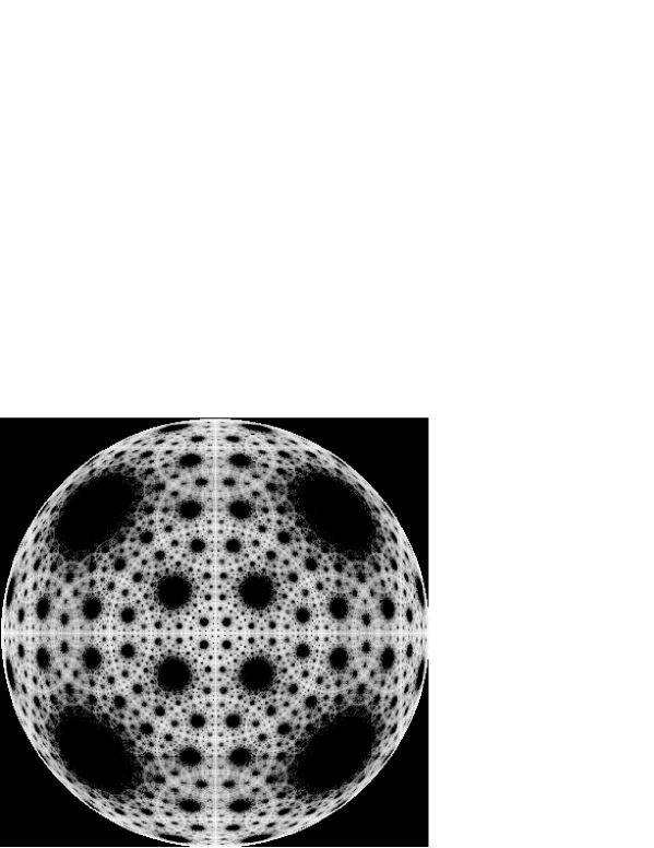
Figure 1: Quantum Octahedron. 100,000,000 jumps on ${\bf P}_{1}({{\mathbb{C}}})$, $\epsilon=0.58$

This fractal figure is in the projective space ${\bf P}_{1}({{\mathbb{C}}})$ and, though impressive, is not what is recorded. What is recorded is a sequence of the detector clicks, together with the times of the clicks $(n_{i},t_{i}).$ The sequence of detector clicks looks pretty much chaotic. Here is an example:

1,1,4,3,1,2,2,1,2,1,5,1,1,5,2,5,2,5,6,6,3,2,2,3,2,5,2,3,1,5,2,5,6,5,6,6,1,2,2,3,
1,3,1,4,4,5,5,5,2,5,5,6,5,6,3,5,3,2,5,4,6,5,5,6,5,4,1,4,6,6,6,3,2,6,6,5,6,5,3,2,
5,2,6,2,2,3,6,2,2,2,2,3,3,2,1,3,4,4,1,1,1,1,4,5,4,4,4,5,4,4,5,5,1,1,1,1,1,4,1,3,
2,2,5,2,2,5,5,6,4,4,3,4,5,4,5,4,4,4,6,5,2,3,2,1,1,3,3,1,5,5,5,6,3,5,6,4,5,2,2,6,
3,2,6,3,1,1,5,4,5,1,4,1,2,5,4,3,3,6,3,3,3,1,4,4,1,5,4,1,5,4,2,5,5,1,4,6,5,4,4,3,
2,3,6,5,5,5,1,5,1,1,5,5,4,6,3,1,1,1,2,2,2,1,2,2,2,5,5,5,2,2,3,6,5,2,5,5,6,4,4,4,
5,4,3,4,6,6,6,3,6,3,3,4,4,6,3,1,1,5,2,5,5,6,3,3,6,1,2,1,2,2,1,1,4,3,3,3,2,1,2,1,
4,3,4,4,4,6,1,3,6,5,1,1,1,2,2,1,1,3,4,4,3,6,2,3,1,2,3,2,5,4,4,1,6,1,1,1,1,4,6,2,
2,5,6,5,1,4,5,6,5,5,6,6,6,6,6,6,6,1,4,4,1,4,3,6,6,2,6,6,4,5,4,4,5,5,4,5,4,6,2,6,
1,5,3,4,5,6,5,6,5,5,6,3,2,3,4,5,1,4,5,4,1,4,1,5,5,6,4,1,1,3,5,1,3,6,6,6,6,6,3,2,
4,6,2,1,5,4,4,4,1,5,5,1,4,5,2,3,2,3,4,5,4,1,4,3,1,3,2,1,3,5,2,2,2,6,6,4,1,5 .

Any information about the initial quantum state seems to be lost rather soon, and is probably irrecoverable from the detectors’ readings due to mixing. There is no general theory yet that would address the problem of recovering probabilistic information about the state of the quantum system and its dynamics from the data recorded by the classical device, except in the limiting cases such as, for instance, when we can take Born’s interpretation limit as discussed above in section II.5.1.

Removing two vertices of the octahedron we get four points that represent our ‘position-momentum’ simultaneous measurement toy model. Since the four remaining vertices are in a plane, which intersects the sphere along a great circle, it is clear that the attractor will be on this circle, and that the fractal pattern will be, in this case, one-dimensional. In Figure 2 we show the path to the attractor, starting with a randomly chosen initial step (left upper corner). The resolution constant $\epsilon$ had to be chosen very small, $\epsilon=0.0045$, since otherwise the state reaches the attractor set on the circle in just few steps. With a much higher resolution ($\epsilon=0.7$) the Cantor set like fractal structure on the circle can be seen. Figure 3 shows one million jumps, first the whole picture, and then $\times 1000$ zoom into the fractal attractor set.

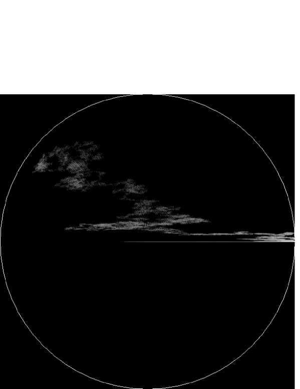
Figure 2: Quantum Square. 200,000 jumps on ${\bf P}_{1}({{\mathbb{C}}})$, $\epsilon=0.0045$

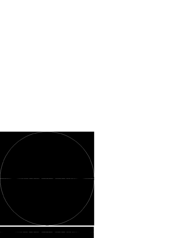
Figure 3: Quantum Square. $10^{6}$ jumps on ${\bf P}_{1}({{\mathbb{C}}})$, $\epsilon=0.7$. The whole picture and $\times 1000$ zoom. The square is located on the plane perpendicular to the viewing plane. One of the four vertices is in the center in front.

Figure 4 shows another self-similar picture, representing quantum jumps on ${\bf P}_{1}({{\mathbb{C}}})$ for twenty detectors arranged at the vertices of a regular dodecahedron.

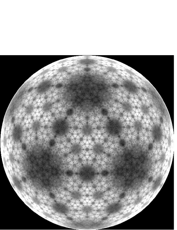
Figure 4: Quantum Dodecahedron. $10^{8}$ jumps on ${\bf P}_{1}({{\mathbb{C}}})$, $\epsilon=0.65$.

IV Quantum Iterated Function Systems

The EQT algorithm generating quantum jumps is similar in its nature to a nonlinear iterated function system (IFS) barnsley (see also peitgen92 and references therein) and, as such, it generically produces a chaotic dynamics for the coupled system. IFS-s are known to produce complex geometrical structures by repeated application of several non-commuting affine maps. The best known example is the Sierpinski triangle

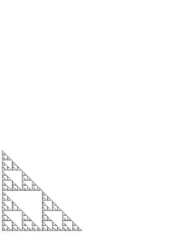
Figure 5: The classical fractal: a Sierpinski Triangle generated by an Iterated Function System.

generated by random application of $3\times 3$ matrices $A[i],i=1,2,3$ to the vector:

$$v_{0}=\left(\begin{array}[]{cc}x_{0}\\ y_{0}\\ 1\end{array}\right),$$ (29)

where $A[i]$ is given by

$$A[i]=\left(\begin{array}[]{ccc}0.5&0&ax_{i}\cr 0&0.5&ay_{i}\cr 0&0&1\end{array}\right)$$ (30)

and $ax_{1}=1.0,ay_{1}=1.0,ax_{2}=1.0,ay_{2}=0.5,ax_{3}=0.5,ay_{3}=1.0.$ (Our $3\times 3$ matrices encode affine transformations – usually separated into a $2\times 2$ matrix and a translation vector.) At each step one of the three transformations $A[i],i=1,2,3$ is selected with probability $p[i]=1/3$. After each transformation the transformed vector is plotted on the $(x,y)$ plane. Theoretical papers on IFSs usually assume that the system is hyperbolic  i.e. that each transformation is a contraction, or, in other words, that the distances between points get smaller and smaller. This assumption is not necessary when the transformations are non-linear and act on a compact space – as is in the case of quantum fractals with which we are dealing. In our case the probabilities assigned to the maps are derived from quantum transition probabilities and thus depend on the actual point, but such generalizations of the IFS’s have been also studied (cf. peigne and references therein). Our algorithm generates quantum fractals, that is self-similar patterns on the complex projective space of pure states of a quantum system.

In a recent paper loslzy Łozinski, Słomczynski and Zyczkowski studied iterated function systems on the space of mixed states, when probabilities that are associated with maps are given independently of the maps, and under assumptions that the maps are invertible. Our maps $g_{\alpha\beta}$ do not have to be invertible, because the probability generating formula (12) assures that probability zero is assigned to a map $\psi\mapsto g_{\alpha\beta}\psi/\|g_{\alpha\beta}\psi\|$ whenever $\|g_{\alpha\beta}\psi\|=0.$

V Open Problems in EQT

There are two kinds of open problems in EQT: those dealing with the developing theory and its applications, and those related to its very foundations. Let us start with questions of the first kind. The original motivation for creating EQT was our dissatisfaction with the rigor of Hawking’s derivation of the black hole radiation formula. The way the classical gravitation field was coupled to a quantum field, with back reaction of the quantum field on classical gravitation, was, in our opinion, highly unsatisfactory. Then there was gravity itself, where the ten components of the metric tensor split naturally into a scalar field $\Phi$ that defines the volume form, and the nine components that define the conformal (i.e. light cone) structure of space-time. A first attempt in quantizing gravity would be quantizing $\Phi$, and leaving the conformal structure at the classical level, yet coupled to the quantized $\Phi$ with a back-action. Although EQT evolved and matured since its birth in 1993, so that we can deal now with infinitely many degrees of freedom and continuous spectra, the two original motivating problems have not yet been modeled within EQT. Also the problem of formulating EQT strictly within the algebraic framework is still waiting for implementation.

Concerning the foundational problems, the number one problem is the derivation of EQT from a set of primitive and easily understandable assumptions. There are several options here and we would like to comment on some of them.

V.1 Environmentally Induced Decoherence

Following the ideas introduced by Gell-Mann, Hartle, Zurek, Zeh and others (see gellhart93 ; zurek91 ; zurek93 ; giulini96 ; zeh01 Blanchard and Olkiewicz blaolk03 tried to rigorously derive the emergence of classical degrees of freedom from particular types of quantum dynamics. The main problem with this kind of an approach is that it uses the undefined, somewhat magical, term ‘environment’. How to split the universe into ‘the system’ and ‘its environment’ is never discussed. If the splitting happens only in the brain of a physicist, the phrase ‘dynamically induced’ is somewhat exaggerated. The point is that the authors start with the assumed open system dynamics and Liouville equation without ever discussing how Schrödinger’s dynamics can ‘dynamically’ deform from an automorphic to a dissipative form. The formal operations, like splitting into a tensor product and taking a conditional expectation value are purely mathematical and have nothing to do with real, physical, dynamical processes. As we mentioned in the introductory part, the very use of the term ‘environment’, without a rigorous definition of the term, is as useless as the use of the term measurement, without being able to provide its formal definition. Any attempt to derive decoherence as a limiting procedure fails to address the problem of events happening in finite time, with the system reacting to the events that happen.

V.2 Bohmian Mechanics

Bohmian mechanics (see bohmhiley ; duerr ) assumes that the classical degrees of freedom – positions and momenta of the particles evolve in a modified potential, determined by the quantum wave function. This theory needs a preferred basis, like, for instance, the coordinate basis. But in the case of pure spin no such preferred basis exists and there is no way in which it can be dynamically selected in a generic case. One can try to argue that the eigenvalue decomposition of a given density matrix provides such a basis, but even this reasoning fails when the density matrix eigenvalues are degenerate.

V.3 Infrared Sectors

If we believe in quantum field theory and if we are ready to take a lesson from it, then we must admit that one Hilbert space is not enough, that there are inequivalent representations of the canonical commutation relations, that there are superselection sectors associated to different phases. In particular there are inequivalent infrared representations associated to massless particles (cf. roep70 and references therein). Then classical events would be, for instance, soft photon creation and annihilation events. That idea has been suggested by Stapp stapp85a ; stapp85b some twenty years ago, and was analyzed in a rigorous, algebraic framework by D. Buchholz buch94a .

Another possibility is that not only photons, but also long range gravitational forces may take part in the transition from the potential to the actual. That hypothesis has been expressed by several authors (see e.g. contributions of F. Károlyházy et al., and R. Penrose in penr85 ; also L. Diosi diosi89 ).

V.4 Deformation Quantization

A large part of our understanding of quantum theory comes through the idea of ‘quantization’. For instance, we take a classical Hamiltonian system on a phase space $M$, typically $M\approx{\mathbb{R}}^{2n}$, and we deform the product $fg$ on the space of $C^{\infty}$ functions on $M$ into a new, non-commutative product $f\star_{\lambda}g$, so that we recover the classical structure for $\lambda\rightarrow 0$ (see bffls1 ; bffls2 for a review). It is in this way that we are able to interpret algebraic objects of quantum theory, by relating them to the well understood objects of classical Hamiltonian dynamics. Flato and Sternheimer suggested fs97 that EQT may be, perhaps, derived in a similar way, via deformation quantization of a classical dissipative (and thus non-Hamiltonian) non-Hamiltonian structure, so that the transition operators $g_{\alpha\beta}$ of EQT can be traced back to well understood classical objects. Deformation quantizations of generalizations of standard Poisson structures and of Hamiltonian dynamics has indeed been developed, mainly with applications based on Nambu mechanics df97 ; fds97 , and quantization of classical dissipative structures has been studied via generalized canonical quantization enz94 ; tarasov01a ; tarasov01b . Yet, until now, the program of quantizing only a part of the system, while the other part remains classical, and relating the result to the formal scheme of EQT remains open.

V.5 Natural Mathematical Constructions

Temporal evolution of a non-dissipative quantum system is described by a one-parameter group of automorphisms of its algebra of observables. It was a surprising discovery when Tomita-Takesaki theory allowed us to naturally associate such a group with each faithful normal state (or, more generally, weight) of the algebra. Connes and Rowelli conrov94 speculated that the modular group of automorphisms of the equilibrium thermal state of the universe provides a quantum dynamics at a fundamental level, a dynamics that defines, by itself the very ‘rate of flow of time’. It is quite possible that by a generalization of the Tomita-Takesaki scheme natural semigroups of completely positive maps can be associated to certain states of von Neumann algebras. If so, then natural examples of EQT dynamics can be produced via pure algebraic means. Some of these example may have a physical interpretation and application to fundamental structures of physics.

V.6 Concluding Remarks

One of the reviewers of the early version of this paper wrote:

“…it is not clear why this approach is more well-founded than ordinary non-relativistic quantum mechanics, nor does the author take account of the fact that most shortcomings of that theory disappear in relativistic quantum field theory.”

In my view this is a typical misunderstanding, shared by many of those physicists who work on difficult technical problems of relativistic quantum fields, and do not follow the discussion about the foundations of quantum theory and its philosophical and interpretational problems. Relativistic quantum field theory not only is of no help in resolving the measurement problem, but, instead, makes it even more profound. R. D. Sorkin discussed some the issues involved in sorkin , where he argues that the standard Hilbert space approach leaves relativistic quantum fields “with no definite measurement theory, removing whatever advantages it may have seemed to possess vis a vis the sum-over-histories approach, and reinforcing the view that a sum-over-histories framework is the most promising one for quantum gravity.” Algebraic quantum field theory is not better in this respect, as measurements are there never defined, and no event ever happens in a finite time. In blaja98a we wrote:

Meaningless infinities of relativistic quantum field theory tell us that something is seriously wrong with our theoretical assumptions. In our opinion, the value of a theory consists not in that it can explain the technique by which the fabric is woven on the loom of Nature, but that it can explain the patterns of the weaving, the Weaver and perhaps the motivations behind the weaving.

Facts cannot be understood by being crafted into a summary or a formula - they can only be understood by being explained. And, understanding is not the same as ‘knowing.’ Quantum Theory, as any other theory, has a finite region of validity - when attempts are made to apply it beyond these limits - we get either nonsense or no answer at all. Quantum theory, in its orthodox version, cannot even be applied to an individual system - like the Universe we live in and experience. We want to discover ‘why’ in addition to ‘what’ regarding the order of the universe in which we find ourselves. We wish to discover why ‘this’ MUST be so, rather than ‘that;’ why Nature does what she does and how. We want to uncover and understand the Laws of Nature, not just the ‘rules of thumb’.”

A typical application of EQT would be, for instance, a dynamical phase transition in the early universe. Recently a hypothesis has been advanced that the universe should be described by a KMS state at the Planck scale (cf. ibog02 and references therein) and that there is a signature fluctuation at this scale. Such a phenomenon can not be described within the standard quantum theory, as it involves ‘events’ and it applies to ‘time itself’. Moreover, KMS condition on a state implies automatically stationarity, therefore the universe would always persist in its original thermodynamic equilibrium. The only way out of an equilibrium is via a quantum jump, using a mechanism analogous to the one described above. Such a jump, or a sequence of jumps, could lead not only to a new phase, but also to self-similarity that is nowadays being observed in the Universe dalpino95 .

In EQT all the probablistic interpretations of quantum theory are derived from the dynamics. In particular, it makes no sense to ask the question ‘what would be a distribution of observed values of an observable’ without adding the appropriate terms to the evolution equation. It is because of the dynamical treatment of the measurement that leads to events and information transfer in finite time, with a feedback, that EQT allows us to answer more questions and to analyze experimental situations that the Standard Quantum Theory seems to exclude from its consideration – like the simultaneous measurement of several noncommuting observables. In this case, as has been explained in this paper, measurement results exhibit chaotic and fractal behaviour.

VI Acknowledgments

The author thanks QFS, Inc for support, and to Eric Leichtnam and Oscar Garcia-Prada for invitation to the workshop Géométrie et Physique, CIRM, Marseille. Thanks are also due to Palle Jorgensen for his encouragement and helpful comments, and to my wife Laura for reading the manuscript.

References

- (1) J. von Neumann, Mathematische Grundlagen der Quantenmechanik (Springer, Berlin, 1932).
- (2) A. Jadczyk, On Quantum Jumps, Events and Spontaneous Localization Models, Found. Phys. 25, 743–762 1995)
- (3) J. Bell, Towards an exact quantum mechanics, in S. Deser and R. J. Finkelstein (eds)Themes in Contemporary Physics II. Essays in honor of Julian Schwinger’s 70th birthday, (World Scientific, Singapore 1989)
- (4) J. Bell, Against measurement, in Sixty-Two Years of Uncertainty. Historical, Philosophical and Physical Inquiries into the Foundations of Quantum Mechanics, Proceedings of a NATO Advanced Study Institute, August 5-15, Erice, Ed. Arthur I. Miller, NATO ASI Series B vol. 226 , (Plenum Press, New York 1990)
- (5) J. Bell, On the impossible pilot wave, in bell86
- (6) J. Bell, Six possible worlds of quantum mechanics, in Speakable and unspeakable in quantum mechanics, (Cambridge University Press, 1987)
- (7) J. Bell, Beables for quantum theory, in bell86
- (8) John A. Wheeler, Delayed–Choice Experiments and Bohr’s Elementary Quantum Phenomenon in Proc. Int. Symp. Found. of Quantum Mechanics, (Tokyo 1983), pp. 140–152
- (9) John A. Wheeler, It From Bit, in Proceedings 3rd International Symposium on Foundations of Quantum Mechanics, (Tokyo, 1989)
- (10) R. Ingarden and M. Grabowski, Mechanika Kwantowa, in Polish, (PWN, Warszawa, 1989)
- (11) M. Ozawa, Controlling Quantum State Reduction, Phys. Lett. A 282, 336 (2001).
- (12) M. Ozawa, Position measuring interactions and the Heisenberg uncertainty principle, Phys. Lett. A 299, 1 (2002).
- (13) M. Ozawa, Universally valid reformulation of the Heisenberg uncertainty principle on noise and disturbance in measurement, Phys. Rev. A 67, 042105 (2003).
- (14) M. Ozawa, Uncertainty Relations for Joint Measurements of non-commuting Observables, eprint archive quant-ph/0310070
- (15) Ozawa, M.: Uncertainty principle for conservative measurement and computing, eprint archive quant-ph/0310071
- (16) H. P. Robertson, The uncertainty principle Phys. Rev. 34, 163-164 (1929).
- (17) E. H. Kennard, Zur Quantenmechanik einfacher Bewegungstypen Z. Phys. 44, 326-352 (1927)
- (18) L. E. Ballentine, The Statistical Interpretation of Quantum Mechanics. Rev. Mod. Phys. 42, 358-381 (1970).
- (19) A. Peres, Quantum Theory: Concepts and Methods (Kluwer Academic, Dordrecht, 1993)
- (20) Ph. Blanchard, and A. Jadczyk, How and When Quantum Phenomena Become Real, in Z. Haba et all. (eds) Proc. Third Max Born Symp., Stochasticity and Quantum Chaos, Sobotka 1993, pp. 13–31, (Kluwer Publ. 1994)
- (21) R. Olkiewicz, Some mathematical problems related to classical-quantum interactions, Rev. Math. Phys. 9 (1997), 719
- (22) Ph. Blanchard, R. Olkiewicz, Interacting quantum and classical continuous systems I. The piecewise deterministic dynamics, J. Stat. Phys. 94, 913 (1999)
- (23) Ph. Blanchard, R. Olkiewicz, Interacting quantum and classical continuous systems II. Asymptotic behavior of the quantum system, J. Stat. Phys. 94, 933 (1999)
- (24) R. Olkiewicz, Dynamical semigroups for interacting quantum and classical systems, J. Math. Phys. 40, 1300 (1999)
- (25) R. Alicki and K. Lendi, Quantum Dynamical Semigroups and Applications, Lect. Notes Phys. 286, 1987
- (26) R. Alicki, Invitation to quantum dynamical semigroups, Lecture given at the 38 Winter School of Theoretical Physics, Ladek, Poland, Feb. 2002, eprint no arXiv:quant-ph/0205188
- (27) G. G. Emch, Algebraic methods in Statistical Mechanics and Quantum Field Theory, (Wiley - Interscience, New York 1972)
- (28) N. P. Landsman, Algebraic Theory of Superselection Sectors and the Measurement Problem in Quantum Mechanics, Int. J. Mod. Phys. A 6 (1991), 5349-5371
- (29) M. H. Davis, Markov models and optimization, Monographs on Statistics and Applied Probability, (Chapman and Hall, London 1993)
- (30) Ph. Blanchard, A. Jadczyk and R. Olkiewicz, Completely Mixing Quantum Open Systems and Quantum Fractals, Physica D: Nonlinear Phenomena, 148 (3-4), 227–241 (2001)
- (31) E. Christensen and D. Evans, Cohomology of operator algebras and quantum dynamical semigroups, J. London. Math. Soc. 20, 358–368 (1978)
- (32) V. Gorini, A. Kossakowski and E. C. G. Sudarshan, Completely positive dynamical semigroups of N–level systems, J. Math. Phys. 17, 821–825 (1976)
- (33) G. Lindblad, On the Generators of Quantum Mechanical Semigroups, Comm. Math. Phys. 48, 119–130 (1976)
- (34) W. B. Arveson, Subalgebras of –algebras, Acta Math. 123, 141–224 (1969)
- (35) W. F. Stinespring, Positive functions on -algebras, Proc. Amer. Math. Soc. 6, 211-216 (1955)
- (36) A. Jadczyk, G. Kondrat and R. Olkiewicz, On uniqueness of the jump process in quantum measurement theory, J. Phys. A 30, 1-18 (1996)
- (37) Ph. Blanchard, and A. Jadczyk, Time of Events in Quantum Theory, Helv. Phys. Acta 69, 613–635 (1996) , also available as quant-ph/9602010
- (38) J. G. Muga, I. L. Egusquiza, J. A. Damborenea, and F. Delgado, Bounds and enhancements for the negative scattering-time delays, Phys. Rev. A 66, 042115 (2002)
- (39) J. P. Palao, J. G. Muga and A. Jadczyk, Barrier traversal times using a phenomenological track formation model, Phys. Lett. A 233, 227-232 (1997)
- (40) A. Ruschhaupt, A Relativistic Extension of Event-Enhanced Quantum Theory, J. Phys. A: Math. Gen. 35, 9227-9243 (2002)
- (41) A. Ruschhaupt, Relativistic Time-of-Arrival and Traversal Time, J. Phys. A: Math. Gen. 35, 10429-10443 (2002)
- (42) A. Peres, Classical interventions in quantum systems, Phys. Rev. A 61, 022117 (2000)
-
(43)
A. Jadczyk, Particle Tracks, Events and Quantum
Theory, Progr. Theor. Phys. 93, 631–646 (1995)
(A model of particle tracks using a continuous medium of detectors. Gives GRW ‘spontaneous localization’ model as a particular case.) - (44) Ph. Blanchard and A. Jadczyk, On the Interaction Between Classical and Quantum Systems, Phys. Lett. A175, 157-164 (1993) (The very first paper, describing the method of coupling of a quantum and of a classical system via dynamical semigroup. At that time we didn’t yet know about piecewise deterministic processes.)
- (45) A. Jadczyk, Topics in Quantum Dynamics, in Proc. First Caribb. School of Math. and Theor. Phys., Saint–Francois–Guadeloupe 1993, Infinite Dimensional Geometry, Noncommutative Geometry, Operator Algebras and Fundamental Interactions, ed. R.Coquereaux et al., (World Scientific, Singapore 1995) ( A review paper. Describes the PDP process. States the problem: “How to determine state of an individual quantum system?” Describes a process on which later was adapted for generation of quantum fractals.)
- (46) K. Popper, Unended Quest. An intellectual Autobiography, (Routledge, London 1993)
- (47) H. Putnam, Quantum Mechanics and the Observer, Erkenntnis 16, 193 (1981)
- (48) N. P. Landsman, Observation and superselection in quantum mechanics, Stud. Hist. Phil. Mod. Phys. 26, 45-73 (1995)
- (49) G. W. Mackey, Unitary Group Representations in Physics, Probability, and Number Theory, (Benjamin, New York 1978)
- (50) V. S. Varadarajan, Geometry of Quantum Theory, (Springer 1985)
- (51) A. Jadczyk and R. Öberg, Quantum Jumps, EEQT and the Five Platonic Fractals, Preprint http://arXiv.org/abs/quant-ph/0204056
- (52) M. F. Barnsley, Fractals everywhere, (Academic Press, San Diego 1988)
- (53) H-O. Peitgen, J. Hartmut and D. Saupe, Chaos and Fractals. New Frontiers of Science, (Springer, New York, 1992)
- (54) Marc Peigné, Iterated Function Systems and spectral decomposition of the associated Markov operator, Preprint U.R.A. C.N.R.S. 305, Prépublication 93 -24, Novembre 1993
- (55) G. Casati, Quantum mechanics and chaos, in: M. J. Gianoni, A. Voros and J. Zinn-Justin (eds), Chaos and Quantum Physics, (North Holland, 1991)
- (56) G. Casati, G. Maspero and D. L. Shepelyansky, Quantum fractal eigenstates, Physica D 131 (1999), 311-316
- (57) A. Lozinski, K. Zyczkowski and W. Slomczynski, Quantum Iterated Function Systems, Phys. Rev. E 68 (2003), 046110 Preprint quant-ph/0210029
- (58) M. Gell-Mann and J. B. Hartle, Classical Equations for Quantum Systems, Phys. Rev. D 47, 3345 (1993),
- (59) D. Giulini et al. (Eds.), Decoherence and The Appearance of a Classical World in Quantum Theory, (Springer, Berlin, 1996)
- (60) H. D. Zeh, The Physical Basis of The Direction of Time, 4th ed., (Springer, Berlin, 2001)
- (61) W. H. Zurek, Decoherence and the transition from quantum to classical, Physics Today 44, 36 (1991).
- (62) W. H. Zurek, Preferred states, predictability, classicality and the environment-induced decoherence, Progress of Theoretical Physics 89, 281-312 (1993).
- (63) Ph. Blanchard, R. Olkiewicz, Decoherence Induced Transition from Quantum to Classical Dynamics, Rev. Math. Phys. 15, 217-243 (2003)
- (64) K. Berndl, M. Daumer, D. D rr, S. Goldstein, N. Zanghi, A Survey on Bohmian Mechanics, Nuovo Cim. B110 (1995) 737-750
- (65) D. Bohm and B. J. Hiley, The Undivided Universe, (Routledge, London, 1993)
- (66) G. Roepstorf, Coherent Photon States and Spectral Condition, Commun. Math. Phys 19 301–314 (1970)
- (67) H. P. Stapp, On the Unification of Quantum Theory and Classical Physics, in Lahti, P., and Mittelstaedt, P. (eds), Symposium on The Foundations of Modern Physics, (World Scientific, 1985)
- (68) H. P. Stapp, Einstein Time and Process Time, in Griffin, D.R. (ed.): Physics and the Ultimate Significance of Time, (State University of New York Press, 1986)
- (69) D. Buchholz, Gauss’ law and the infraparticle problem, Phys. Lett. B 174 331–334 (1986)
- (70) R. Penrose and C. J. Isham,(eds) Quantum Concepts in Space and Time, (Clarendon Press, Oxford 1986)
- (71) L. Diosi, Models for universal reduction of macroscopic quantum fluctuations, Phys. Rev. A 40,1165–1174 (1989)
- (72) F. Bayen, M. Flato, c. Fronsdal, A. Lichnerowicz and D. Sternheimer, Deformation Theory and Quantization. I. Deformation of Symplectic Structures, Ann. Phys. 111, 61-110 (1978)
- (73) F. Bayen, M. Flato, c. Fronsdal, A. Lichnerowicz and D. Sternheimer, Deformation Theory and Quantization. II. Physical Applications, Ann. Phys. 111, 111-151 (1978).
- (74) M. Flato and D. Sternheimer, Private communication
- (75) G. Dito and M. Flato, Generalized Abelian Deformations: Application to Nambu Mechanics, Lett.Math.Phys. 39, 107-125 (1997).
- (76) M. Flato, G. Dito and D. Sternheimer, Nambu Mechanics, -ary Operations and their Quantization, in D. Sternheimer, J. Rawnsley and S. Gutt (eds), Proceedings of the Ascona Meeting, Deformation Theory and Symplectic Geometry, June 1996, Mathematical Physics Studies, vol 20 (1997) (Kluwer, 1997).
- (77) C. P. Enz, Hamiltonian Description and Quantization of Dissipative Systems, Found. Phys. 24, 1281-1292 (1994).
- (78) V. E. Tarasov, Quantization of non-Hamiltonian Systems, Theoretical Physics 2., 150-160 (2001) .
- (79) V. E. Tarasov, Quantization of non-Hamiltonian and Dissipative Systems, Physics Letters A 288. No.3/4. (2001) pp.173-182.
- (80) A. Connes, C. Rovelli, Von Neumann Algebra Automorphisms and Time-Thermodynamics Relation in General Covariant Quantum Theories, Class.Quant.Grav. 11, 2899-2918 (1994).
- (81) R. D. Sorkin, Impossible Measurements on Quantum Fields, in Directions in General Relativity: Proceedings of the 1993 International Symposium, Maryland, Vol. 2: Papers in honor of Dieter Brill, pages 293-305, Bei-Lok Hu and T.A. Jacobson editors, (Cambridge University Press, 1993)
-
(82)
Ph. Blanchard, and A. Jadczyk,
A Way Out of the Quantum Trap,
in it Open Systems and Measurement in
Relativistic Quantum Theory , H. P. Breuer and F. Petruccione
(Eds.), (Lecture Notes in Physics, Springer-Verlag, 1999)
(A review paper. With FAQ on EQT.) Preprint quant-ph/9812081 - (83) I. Bogdanoff, The KMS State of Spacetime at the Planck Scale, Chin. J. Phys. 40, 149–158 (2002).
- (84) E. M. de Gouveia Dal Pino, A. Hetem, J.E. Horvath, C. A. W. de Souza, T. Villela, J. C. N. de Araujo, Evidence for a Very Large-Scale Fractal Structure in the Universe from Cobe Measurements, Astrophysical Journal Lett. 442, L-45-L48 (1995).