Collapsing the Wavefunction of a Baseball

Abstract

The transition from microscopic to macroscopic in quantum mechanics can be seen from various points of view. It is often not merely a transition from quantum to classical mechanics in the sense of the Correspondence Principle. The fact that real macroscopic objects like baseballs are composites of an extremely large number of microscopic particles (electrons, protons etc.) is a complicating factor. Here such composite objects are studied in some detail and the Copenhagen interpretation is applied to them. A computer game model for a simplified composite object is used to illustrate some of the issues.

1 Introduction

Since the advent of quantum physics about a century ago, physicists have valiantly tried to understand it at an intuitive level. However, our normal intuition is developed and exercised almost exclusively in the classical world of macroscopic objects. So any attempt at understanding quantum mechanics intuitively is predisposed to fail. Nonetheless, we keep trying in the hope of at least partial success.

I remember one such attempt in my first quantum physics course in college. We learnt that the longer the wavelength of a wave, the easier it is to detect its wave nature (using diffraction experiments). Diffracting sound waves is almost trivial, but for light waves we need one or more extremely narrow slits (gratings with spacing of the order of 10^-6 m). For X-rays and electrons the grating pattern has to be finer still (of the order 10^-10 m as found in crystals). Now, what about the diffraction of a “beam” of baseballs? Using the de Broglie formula, for a nominal baseball momentum, one computes slit widths needed to diffract such a beam to be of the order of 10^-34 m! The impossibility of such a grating is given as the reason why baseballs are not seen to diffract.

However, a closer look at such reasoning shows serious flaws. If slit widths of the order of 10^-34 m were actually possible, there is still no way one can imagine baseballs getting through them (baseballs are simply too big!). The transition from an electron to a baseball is not merely a change in mass. An electron is a structureless fundamental particle whereas a baseball is a composite of an enormous number of fundamental particles bound together. This means that an electron has no measure of spatial extent or size but the baseball has a well defined measure of size based on equilibrium distances between component particles. For the baseball to squeeze through a narrow slit, the distances between its component particles must be decreased dramatically. This would require ridiculously high energies. The electron being structureless will have no problems squeezing through any slit. Hence, the composite nature makes the baseball qualitatively very different. A proton is a composite of only three objects and already it shows a magnetic moment and scattering cross sections (Bjorken scaling) that are very different from structureless particles.

So, here I shall take a closer look at the quantum mechanics of composite objects. In particular, the process of position observation and the resulting collapse of wavefunctions of composites like baseballs will be studied. For this purpose, a sharpened form of the Copenhagen interpretation will be used. Also, a computer game based on these ideas will be used to provide some of that illusive “intuitive” understanding.

2 Observing a baseball

When the catcher observes the position of a baseball, it is not a direct measurement of the center of mass (CM). Hence, the baseball wavefunction does not collapse to an eigenstate of CM position. Consequently, the momentum does not become particularly uncertain. To verify these statements, let us look at this process of baseball position observation in some detail.

When the catcher “sees” the baseball, he/she makes myriads of observations – mostly energies and momenta of photons scattered from the surface of the ball. Photon energies are determined by the colors observed. The colors also help distinguish the ball from its background thus allowing the catcher to gaze in the direction of the ball. This direction gives the directions of the photon momenta. The magnitudes of photon momenta are known from the colors. Hence, the photon momenta are known both in magnitude and direction. The momentum of a specific photon locates the position of the surface electron that scattered it. This kind of position measurement of different components of the surface of the ball allows the estimation of the CM position without actually measuring it. Thus total momentum does not become unduly uncertain.

The above explanation is significantly different from that offered in standard introductory courses where the uncertainty in CM position is estimated to be the diameter of the ball. Then the uncertainty in total momentum is computed using the uncertainty principle. This also shows that total momentum uncertainty is not alarmingly large.

3 Keeping up with Copenhagen

In the last section it was argued that CM position is estimated from position measurements of surface particles (mostly electrons). However, even surface electron positions are not being measured directly. They are measured through the photons they scatter. So, should the wavefunction of such a surface electron collapse?

There may be some controversy about this question. Some (following Wigner) give the Copenhagen interpretation a somewhat anthrocentric tilt. They say that wavefunction collapse is achieved only by an observation made by a conscious observer[1, 2, 3] and as no conscious observer observes those surface electrons directly, their wavefunctions do not collapse. However, this understanding can quickly drag physics into metaphysics. The contentious definition of consciousness becomes central to the argument.

On the other hand, if we were to consider an observer to be just a large collection of particles capable of recording data by selecting particle states (brain chemistry)[1, 4], our understanding can be based on known physics. So, the observer is a macroscopic recorder that stores information in multiple particle states (often redundantly) as a consequence of an observation. The photon scattered from an electron is a microscopic analog of the same thing[1, 5]. It changes its own state due to the scattering and hence, records information about the scattering agent (the electron). Thus the scattering of the photon is a measurement of electron position and must result in the collapse of the electron wavefunction.

Getting back to the baseball, we see that the indirect estimation of the baseball position requires the collapse of wavefunctions of a negligibly small number of surface electrons. Hence, for all practical purposes, the baseball is unaffected by the measurement. This justifies the classical model of the baseball. The few electrons that suffer wavefunction collapse develop high momentum uncertainties and may even escape the binding forces that attach them to the ball. The computer model discussed later shows this effect.

4 Dynamics of composite objects

Macroscopic objects like baseballs have a very large number of degrees of freedom due to their large number of component particles. When the position of one of these particles (say an electron) is measured, the whole baseball wavefunction collapses to an eigenstate of position of just that one electron for a specific position eigenvalue. However, such a baseball eigenstate must be highly degenerate as its dependence on all other particle positions can be anything. The collapsing process needs to select one of these many degenerate states. To understand this we need to study the dynamics of a composite object with a large number of component particles.

The simplest composite would be a bound system of two particles. This system has been studied extensively both classically and quantum mechanically as seen in introductory texts[6, 7, 8]. However, the two-particle case is a special one. For most realistic interaction potentials, this can be separated into two independent one-particle problems – one a free particle (CM position) and the other a particle interacting with a background potential.

A similar separation for three or more interacting particles is unknown. This makes analytical solutions for such systems difficult. However, numerical solutions are quite straightforward (although time consuming). Hence, I shall outline such a numerical approach for the non-relativistic quantum case. It can be implemented on a PC with some approximations. This implementation, in spite of the approximations, provides physical insight into the wavefunction collapse process. It can simulate component particle detection by mouse clicks (turning the simulation into a game).

Let the composite object consist of $N$ mutually interacting distinguishable particles with positions ${\bf q}_{i}$ and momenta ${\bf p}_{i}$ ($i$=1, 2, …, $N$). Let the hamiltonian for this object be $H(\{{\bf q}_{i}\},\{{\bf p}_{i}\})$ and its wavefunction at time $t$ be $\psi(\{{\bf q}_{i}\},t)$. Then the integral form of the time dependent Schrödinger equation gives the time development of the wavefunction to be

$$\psi(\{{\bf q}_{i}\},t)=e^{-iHt/\hbar}\psi(\{{\bf q}_{i}\},0).$$ (1)

While no observations are made on the object, the above equation provides the wavefunction at anytime. It can also be written as

$$\psi(\{{\bf q}_{i}\},t)=\lim_{\Delta t\rightarrow 0}(1-iH\Delta t/\hbar)^{n}\psi(\{{\bf q}_{i}\},0),$$ (2)

where $n$ is an integer and $n\Delta t=t$. For a numerical evaluation, $\Delta t$ can be chosen to be small but finite. Then the time development of $\psi$ can be computed in time steps of $\Delta t$. Using equation (2), it can be seen that the values of $\psi$ at successive time steps are related as follows.

$$\psi(\{{\bf q}_{i}\},t)=(1-iH\Delta t/\hbar)\psi(\{{\bf q}_{i}\},t-\Delta t).$$ (3)

This can be used for an iterative computation of $\psi$ if the initial value is known. Although this method becomes unstable for large numbers of time steps[12], it is adequate for the present application. Here, after every few steps, the wavefunction will be collapsed. This prevents the solution from becoming unstable.

An iterative computation using short time steps also allows computer animation of the time development. The wavefunction, at each time step, provides a frame for animation.

If a particle detector detects the $k^{\mbox{th}}$ particle in a small region $R$, it will be with a probability $P_{k}$ given by

$$P_{k}=\int_{R}d^{3}{\bf q}_{k}\int_{-\infty}^{\infty}\int_{-\infty}^{\infty}\cdots\int_{-\infty}^{\infty}\prod_{j\neq k}d^{3}{\bf q}_{j}\psi^{*}(\{{\bf q}_{i}\},t)\psi(\{{\bf q}_{i}\},t).$$ (4)

If the particle is actually detected, the wavefunction must collapse to

$$\psi_{c}(\{{\bf q}_{i}\},t)=A\Delta_{R}({\bf q}_{k}-{\bf q}_{0})\psi(\{{\bf q}_{i}\},t),$$ (5)

where $\Delta_{R}({\bf q}_{k}-{\bf q}_{0})$ is a sharply peaked function that is nonzero only in the region of detection $R$ centered about the position ${\bf q}_{0}$. The detailed form of this function depends on the detector sensitivity in the region $R$. In the limit $R\rightarrow 0$, it is the Dirac delta function:

$$\lim_{R\rightarrow 0}\Delta_{R}({\bf q}_{k}-{\bf q}_{0})=\delta^{3}({\bf q}_{k}-{\bf q}_{0}).$$ (6)

The constant $A$ is needed to renormalize $\psi$ after the collapse. It is to be noted that the collapsed wavefunction is highly degenerate because only one particle position is measured and the other particles could be in many different states without changing this measurement. So one needs to select a linear combination of these degenerate states to be $\psi_{c}$. This is done by setting the amplitudes of the members of the degenerate set in the same proportion as before the collapse. Equation (5) does this effectively by keeping the dependence on all ${\bf q}_{i}$ other than ${\bf q}_{k}$ the same as before the collapse.

After the collapse, $\psi$ is replaced by $\psi_{c}$ and the time development continued as given by equation (1) until the next collapse.

When this process of time development of the wavefunction and its occasional collapse is computer animated and displayed on screen, many interesting effects are observed. But the overall visual effect is what one looks for. It brings us a little closer to that much desired “intuitive understanding”.

5 The binding potential

The algorithm of the previous section is general for any arbitrary hamiltonian $H$. For a specific composite object, the interparticle binding potential needs to be specified. Clearly, we cannot use the binding potential of a real baseball. Even if we actually knew what it is, it would not be a practical choice for numerical computation. So, I choose a potential that is simple but realistic. As all bound particles near equilibrium can be approximated to be in a harmonic (“spring”) potential, I choose a multiparticle harmonic potential for the present computation. Each particle of the composite is assumed to be attached by a spring to a common center. The unextended lengths of the springs are assumed to be zero. This results in the following hamiltonian.

$$H=\sum_{i=1}^{N}\frac{{\bf p}_{i}^{2}}{2m_{i}}+\sum_{i=1}^{N}\frac{k_{i}}{2}({\bf q}_{i}-{\bf q}_{c})^{2},$$ (7)

where $m_{i}$ is the mass and $k_{i}$ the spring constant for the $i^{\mbox{th}}$ particle. ${\bf q}_{c}$ is the position of the common center.

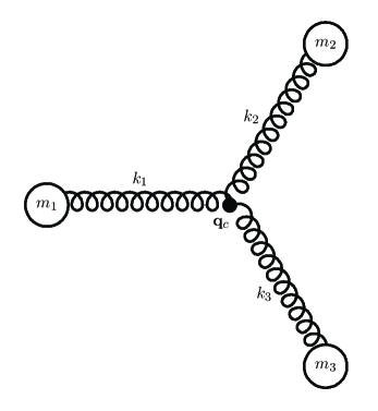
Figure 1: Three particles attached by “springs”

The $N=3$ case of this system can be visualized as in figure 1. As the sum of the internal forces must be zero, the following condition must be satisfied.

$$\sum_{i=1}^{N}k_{i}({\bf q}_{i}-{\bf q}_{c})=0,$$ (8)

which gives

$${\bf q}_{c}=\frac{\sum_{j=1}^{N}k_{j}{\bf q}_{j}}{\sum_{j=1}^{N}k_{j}}.$$ (9)

Hence,

$$H=\sum_{i=1}^{N}\frac{{\bf p}_{i}^{2}}{2m_{i}}+\sum_{i=1}^{N}\frac{k_{i}}{2}\left({\bf q}_{i}-\frac{\sum_{j=1}^{N}k_{j}{\bf q}_{j}}{K}\right)^{2},$$ (10)

where $K=\sum_{j=1}^{N}k_{j}$.

6 Outline of a numerical approach

The computer screen being 2-dimensional, I shall simulate the above N-particle composite in two dimensions. To use standard finite difference methods, the screen space is divided into a matrix of $m$ columns and $n$ rows to produce a total of $m\times n$ points. Although $m$ and $n$ need to be large for accuracy, practical animation on a PC requires that they be small (less than 10 each). Hence, if this method is used to build an animated computer game, $m$ and $n$ must be given small values. This is not a problem as, for the purposes of a game, only qualitative aspects need be displayed.

To solve the Schrödinger equation, boundary conditions must be specified. There are several possible natural choices:

1. Perfectly reflecting boundary conditions.

2. Perfectly absorbing boundary conditions.

3. Periodic boundary conditions.

The perfectly reflecting boundary produces a discontinuity at the boundary that interferes with visualization. The perfectly absorbing boundary allows particles to go off screen, thus making them useless for visualization. The periodic condition seems to be the best for visualization. It identifies the left edge to the right and the bottom edge to the top (toroidal topology). Hence, particle current that disappears on one edge reappears on the opposite edge.

The discrete forms for the $x$ and $y$ components of each coordinate ${\bf q}_{i}$ may be written as

$$q_{ix}=a_{ix}\Delta x,\;\;\;\;q_{iy}=a_{iy}\Delta y,$$ (11)

where $i=1,2,\ldots,N$, $a_{ix}=1,2,\ldots,m$, and $a_{iy}=1,2,\ldots,n$. $\Delta x$ is the mesh width in the $x$ direction and $\Delta y$ is the mesh width in the $y$ direction.

The wavefunction $\psi$, at one instant of time, is a function of all coordinates ${\bf q}_{i}$. So, its discretized form must depend on all $a_{ix}$ and $a_{iy}$. Thus, for numerical computation, $\psi$ is represented by an array of $2N$ dimensions (one for each $a_{ix}$ and $a_{iy}$). In the notation of the C language it would be: $\psi[a_{1x}][a_{1y}][a_{2x}][a_{2y}]\ldots[a_{Nx}][a_{Ny}]$. For the special case of three particles this would be: $\psi[a_{1x}][a_{1y}][a_{2x}][a_{2y}][a_{3x}][a_{3y}]$. For compactness of notation I can write this as: $\psi[a][b][c][d][e][f]$ or $\psi_{a,b,c,d,e,f}$. Then the finite difference form of the operation by the hamiltonian $H$ is found from equation (7) using equation (11) and the following finite difference forms of the ${\bf p}_{i}^{2}$ operators.

$${\bf p}_{1}^{2}\psi_{a,b,c,d,e,f} = -\hbar^{2}\left(\frac{\psi_{a+1,b,c,d,e,f}-2\psi_{a,b,c,d,e,f}+\psi_{a-1,b,c,d,e,f}}{(\Delta x)^{2}}+\right.$$

$$+\left.\frac{\psi_{a,b+1,c,d,e,f}-2\psi_{a,b,c,d,e,f}+\psi_{a,b-1,c,d,e,f}}{(\Delta y)^{2}}\right),$$

$${\bf p}_{2}^{2}\psi_{a,b,c,d,e,f} = -\hbar^{2}\left(\frac{\psi_{a,b,c+1,d,e,f}-2\psi_{a,b,c,d,e,f}+\psi_{a,b,c-1,d,e,f}}{(\Delta x)^{2}}+\right.$$

$$+\left.\frac{\psi_{a,b,c,d+1,e,f}-2\psi_{a,b,c,d,e,f}+\psi_{a,b,c,d-1,e,f}}{(\Delta y)^{2}}\right),$$

$${\bf p}_{3}^{2}\psi_{a,b,c,d,e,f} = -\hbar^{2}\left(\frac{\psi_{a,b,c,d,e+1,f}-2\psi_{a,b,c,d,e,f}+\psi_{a,b,c,d,e-1,f}}{(\Delta x)^{2}}+\right.$$ (12)

$$+\left.\frac{\psi_{a,b,c,d,e,f+1}-2\psi_{a,b,c,d,e,f}+\psi_{a,b,c,d,e,f-1}}{(\Delta y)^{2}}\right).$$

Here the most common finite difference form for second derivatives is used. Generalizing this formula for arbitrary $N$ is tedious but straightforward. Using equations (7), (11), and (12) in equation (3), the wavefunction for successive time steps can be computed. The numerical method chosen here does not maintain normalization of $\psi$. Hence, after each time step computation, $\psi$ must be normalized[12].

Also after each time step computation, the screen image must be updated to provide an animated visual effect. A visually intuitive way of doing this for $N=3$ is to represent each particle by a primary color (red, green and blue). Then, each position on screen (a box of size $\Delta x\times\Delta y$) is colored by a mix of primary colors in proportion to the probabilities of finding the corresponding particles at that position. These probabilities are given by the finite difference form of equation (4):

$$P_{1} = \sum_{c,d,e,f}\psi^{*}_{a,b,c,d,e,f}\psi_{a,b,c,d,e,f},$$

$$P_{2} = \sum_{a,b,e,f}\psi^{*}_{a,b,c,d,e,f}\psi_{a,b,c,d,e,f},$$

$$P_{3} = \sum_{a,b,c,d}\psi^{*}_{a,b,c,d,e,f}\psi_{a,b,c,d,e,f}.$$ (13)

To produce the effect of wavefunction collapse, one uses the mouse button click message to trigger a collapse at the point of clicking. However, clicking the mouse button will collapse the wavefunction for the position of just one of the particles and that too only with a probability given by equation (13). This probabilistic effect can be produced using a random number generator. The wavefunction after the collapse is given by equation (5). The function $\Delta_{R}({\bf q}_{k}-{\bf q}_{0})$ in its discrete form can be chosen as the discrete form of the Dirac delta function:

$$\Delta_{R}({\bf q}_{k}-{\bf q}_{0})=\left\{\begin{array}[]{ll}1,&\mbox{if $a_{kx}=a_{0x}$ and $a_{ky}=a_{0y}$}\\ 0,&\mbox{otherwise},\end{array}\right.$$ (14)

where the integer values $a_{kx}$, $a_{0x}$, $a_{ky}$ and $a_{0y}$ are defined as in equation (11).

7 Some results

It has been demonstrated in an earlier publication[13] that displaying quantum effects in the form of a computer game can provide a useful visual tool for the understanding of quantum mechanics. The formulation of the three particle case of the present problem has inspired another such game[14]. This game illustrates some obvious and some not-so-obvious aspects of composite object quantum mechanics.

As expected, the wavefunction collapse leaves the undetected particles unaffected. Also as expected, the probability profile of each particle spreads with time. What is not-so-obvious is as follows. If we start with one particle in a collapsed state (with no velocity), with time its probability peak moves away from those of the other particles! As the potential function used here is attractive, this is somewhat surprising. However, closer scrutiny can explain this phenomenon.

Consider the standard one-particle harmonic oscillator. Higher energy eigenstates have probability peaks farther away from the origin. This means that particles that start off with higher momenta are likely to have their probability peaks farther away. For the present case, a particle collapsed to its position eigenstate has high probabilities for large momenta and hence, large energy. This makes its probability peak move away from the other particles.

This brings us back to the baseball problem. When the position of a single component particle (electron) is detected, it is likely to escape due to large momentum uncertainty. But the momentum uncertainties of the remaining particles are virtually unaffected by this detection process.

8 Conclusion

For the purpose of quantum mechanical analysis of observation, macroscopic objects like baseballs cannot be treated as just scaled up versions of microscopic objects. Macroscopic objects are made of a large number of microscopic objects tied together by some forces. This composite nature of macroscopic objects gives them properties qualitatively different from microscopic ones. The quantum description of composite objects is in principle straightforward but computationally time consuming. However, some qualitative properties of composites can be observed in a simplified and approximate model implemented as a computer game. In particular, it shows why position observations do not make the total momentum of the composite unduly uncertain.

References

- [1] Griffiths D J 1995 Introduction to Quantum Mechanics, (Prentice Hall) pp 3-5, pp 374-385
- [2] Jammer M 1974 The Philosophy of Quantum Mechanics, (J. Wiley & Sons, New York)
- [3] Wigner E P 1962 The Scientist Speculates (ed. Good I J, Heinemann, London)
- [4] Schrödinger E 1935 Proc. Camb. Phil. Soc. 31 555
- [5] Heisenberg W 1960 Physics and Beyond (Harper & Rowe, New York) pp 60-62
- [6] Goldstein H, Poole C P Jr. and Safko J L 2002 Classical Mechanics (third edition, Addison Wesley)
- [7] Shankar R 1994 Principles of Quantum Mechanics (second edition, Plenum Press)
- [8] Biswas T Quantum Mechanics – Concepts and Applications (available at the URL: www.engr.newpaltz.edu/biswast)
- [9] Whittaker E T 1937 A Treatise on the Analytical Dynamics of Particles and Rigid Bodies (Dover, New York).
- [10] Biswas T 1994 Nuovo Cimento A 107 863
- [11] Biswas T and Rohrlich F 1985 Nuovo Cimento A 88 125
- [12] Press W H, Teukolsky S A, Vetterling W T and Flannery B P 1992 Numerical Recipes in C (second edition, Cambridge University Press) pp 851-853
- [13] Biswas T 2001 Computing in Science and Engineering 3 84. The related game is called “Quantum Duck Hunt” (Microsoft Windows software). It is available at the URL: www.engr.newpaltz.edu/biswast.
- [14] The game discussed here is called “Quantum Focus” (Microsoft Windows software). It is available at the URL: www.engr.newpaltz.edu/biswast.