Electronic address: ]tsujino@es.hokudai.ac.jp Electronic address: ]h.hofmann@osa.org Also at ]PRESTO project, Japan Science and Technology Agency. Electronic address: ]takeuchi@es.hokudai.ac.jp Also at ]CREST project, Japan Science and Technology Agency. Electronic address: ]sasaki@es.hokudai.ac.jp

Distinguishing genuine entangled two–photon–polarization states
from independently generated pairs of entangled photons

Abstract

A scheme to distinguish entangled two–photon–polarization states ($ETP$) from two independent entangled one–photon–polarization states ($EOP$) is proposed. Using this scheme, the experimental generation of $ETP$ by parametric down–conversion is confirmed through the anti–correlations between three orthogonal two–photon–polarization states. The estimated fraction of $ETP$ among the correlated photon pairs is 37$\%$ in the present experimental setup.

Entanglement is one of the key features of quantum theory, and the generation of entangled one–photon–polarization states ($EOP$) by parametric down–conversion has been the focus of much experimental research Mandel88 ; Kwiat95 ; Kwiat99 . Such entangled photon pairs have also been employed in several experiments on quantum information processing and quantum communication ZeilingerBook . At present, there appear to be two ways to expand the concept of entangled photons: increase the number of local systems, or increase the number of photons in the local system. In the former case of multi–party entanglement, single photons are distributed to multiple parties. This case has been realized through the generation of three–party entangled states such as GHZ states GHZ_1 ; GHZ_2 ; GHZ_3 , and various four–party entangled states FourPhotonEntangle . In the latter case, $n$ photons conformed to the same spatiotemporal mode are distributed to each party. The first step in this direction is the generation of entangled two–photon–polarization states ($ETP$).

The two–photon–polarization states can be expressed using a basis of three orthogonal states ThreeStates , exploiting the indistinguishability or bosonic nature of the two photons. Thus, two–photon–polarization states may be used as physical representations of three–level systems. Howell et al. Howell02 recently reported the violation of a Bell’s inequality for spin–1 systems (three–level systems) proposed by Gisin and Peres GisinPeres92 using $ETP$. The quantum mechanical prediction of the maximum value of the conclusion for the $ETP$ is 2.55, whereas the classically predicted maximum is 2. Howell et al. experimentally confirmed the violation of this inequality, obtaining an experimental value of 2.27 $\pm$ 0.02, attributing the result to $ETP$. However, the present authors have found that two independent EOPs, which may have been generated in the same experimental setup, can also violate the Bell’s inequality used by Howell et al., with a value of up to 2.41 for the correlations. This is possible because the correlations in Bell’s inequalities are not a measure of indistinguishability, but rather of non–locality. Thus, the violation of a Bell’s inequality reported by Howell et al. in Howell02 does not require the generation of $ETP$ and an alternative method for obtaining direct evidence of the generation of $ETP$ is desirable.

In this letter, we therefore propose a novel method to distinguish $ETP$ from two independent $EOP$s. In the proposed method, the orthogonality of three two–photon–polarization basis states is checked via the correlations between the two local systems. The experimental generation of $ETP$ using parametric down–conversion can then be evaluated using the proposed method. The results clealy reveal an anti–correlation between the corresponding basis states, indicating the successful generation of $ETP$.

$EOP$ can be generated by pulsed type–II parametric down–conversion Kwiat95 . When one pair of photons is emitted into two modes A and B, the quantum state of the pair is ideally given by

$$|EOP\rangle=(|H\rangle_{A}|V\rangle_{B}-|V\rangle_{A}|H\rangle_{B})/\sqrt{2},$$ (1)

where $H$ and $V$ represent horizontal and vertical polarization. This state has been used in many experiments on quantum information using photons ZeilingerBook . However, in general, multi–pair states are also generated in higher–order processes LamasLinares01 . When two pairs are emitted simultaneously, the quantum state of the pairs is ideally given by

$$|ETP\rangle = \frac{1}{\sqrt{3}}(|HH\rangle_{A}|VV\rangle_{B}$$ (2)

$$- |HV\rangle_{A}|HV\rangle_{B}+|VV\rangle_{A}|HH\rangle_{B}),$$

where $|HH\rangle$, $|HV\rangle$ and $|VV\rangle$ are the three orthogonal basis states of two–photon–polarization states, corresponding to two $H$–polarized photons, one photon $H$–polarized and $V$–polarized each, and two $V$–polarized photons, respectively. Note that these states differ from the simple direct products of two photons, $|H\rangle_{1}\otimes|V\rangle_{2}$, where 1 and 2 denote spatially or temporally independent modes.

The proposed method for distinguishing $ETP$ from two independent $EOP$s is as follows. The basis states of Eq. (2) can be transformed into three orthogonal unpolarized photon states, i.e.,

$$|ETP\rangle = \frac{-1}{\sqrt{3}}(|HV\rangle_{A}|HV\rangle_{B}$$ (3)

$$+ |PM\rangle_{A}|PM\rangle_{B}+|RL\rangle_{A}|RL\rangle_{B}),$$

where

$$|PM\rangle=\frac{1}{\sqrt{2}}(|HH\rangle-|VV\rangle),$$ (4)

$$|RL\rangle=\frac{i}{\sqrt{2}}(|HH\rangle+|VV\rangle).$$ (5)

Here, $P$, $M$, $R$ and $L$ represent plus–diagonal ($|P\rangle=[|H\rangle+|V\rangle]/\sqrt{2}$), minus–diagonal ($|M\rangle=[|H\rangle-|V\rangle]/\sqrt{2}$), right–circular ($|R\rangle=[|H\rangle+i|V\rangle]/\sqrt{2}$) and left–circular ($|L\rangle=[|H\rangle-i|V\rangle]/\sqrt{2}$) polarizations. Thus, $|PM\rangle$ represents a $P$–polarized photon and an $M$–polarized photon generated in the same mode, and $|RL\rangle$ denotes an $R$–polarized photon and an $L$–polarized photon. Note that these three states also form a set of orthogonal basis states ThreeStates .

Consider the case that one of the two photons of Eq. (3), say that in path A, is detected in the $H$–polarized state, and the other photon also in path A is detected in the $V$–polarized state. In this situation, the two–photon–polarization states in mode A would be projected into the $|HV\rangle$ state, and the two–photon–polarization state in mode B would also be projected automatically into the $|HV\rangle$ state due to the entanglement between paths A and B. Consequently, the probability of detecting two photons in mode B in $|RL\rangle$ or $|PM\rangle$ states will be zero. Therefore, in actual experiments, a four–fold coincidence event in which the two photons in either mode are detected with different polarization ($H$ and $V$ in mode A, $P$ ($R$) and $M$ ($L$) in mode B) will never occur for pure state $ETP$. In the following, the number of coincidence events given the same measurement bases is defined as $C_{\parallel}$, and that for different measurement bases is defined as $C_{\perp}$. In the case of ideal pure state $ETP$, the ratio $r=C_{\perp}/C_{\parallel}$ is obviously 0.

Next, consider the case in which two independent $EOP$s described by Eq. (1) are emitted into spatially or temporally separable modes. The state of these two pairs is given by

$$|EOP\otimes EOP\rangle$$ (6)

$$= \frac{1}{\sqrt{2}}(|H\rangle_{A1}|V\rangle_{B1}-|V\rangle_{A1}|H\rangle_{B1})$$

$$\otimes \frac{1}{\sqrt{2}}(|H\rangle_{A2}|V\rangle_{B2}-|V\rangle_{A2}|H\rangle_{B2}),$$

where modes A1 and A2 (B1 and B2) are in the same optical path A (B) but are spatially or temporally distinguishable. For example, when two photons of Eq. (6) in path A are measured in the $H/V$ basis, $|V\rangle_{A1}\otimes|H\rangle_{A2}$, the state in path B will be $|H\rangle_{B1}\otimes|V\rangle_{B2}$ due to the polarization entanglement. Suppose the two photons in modes B1 and B2 are detected in the $R/L$ basis, i.e. $|R\rangle_{B1}\otimes|L\rangle_{B2}$ or $|L\rangle_{B1}\otimes|R\rangle_{B2}$. Since the two photons are independent, the conditional probability for detecting two photons with polarization $|R\rangle$ and $|L\rangle$ when the other two photons in path A are detected with polarization $|H\rangle$ and $|V\rangle$ is $|{}_{B1}\langle R|H\rangle_{B1}{}_{B2}\langle L|V\rangle_{B2}|^{2}+|{}_{B1}\langle L|H\rangle_{B1}{}_{B2}\langle R|V\rangle_{B2}|^{2}=1/2$. Therefore, the ratio $r$ for two independent $EOP$s should be 1/2 even in the ideal case of pure state emission.

Since the correlations between the polarizations in A and B should be maximal for the ideal pure state, it is reasonable to assume that r will be greater or equal to 1/2 in the more general case of mixed state $EOP$s. Specifically, depolarization effects due to experimental imperfections in the alignment of the optical setup will typically increase the value of $r$. For realistic mixed state $EOP$s, we can therefore assume that $r\geq 1/2$ footnote .

These results suggest that the $ETP$ can be distinguished from two independent $EOP$s by measuring the correlation of the three orthogonal polarization basis states. According to the results given above, the following condition indicates the presence of $ETP$ among emitted photons,

$$r<\frac{1}{2}.$$ (7)

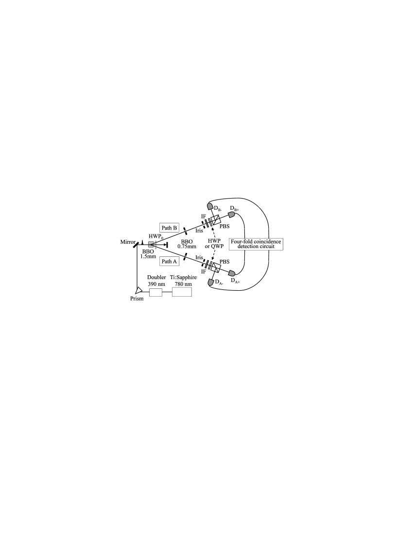
Figure 1: Experimental setup for generation of entangled photon pairs and measurement of polarization correlation between paths A and B. Entangled pairs are generated in a beta–barium borate (BBO) crystal by pulsed parametric down–conversion. $|HV\rangle$, $|RL\rangle$ and $|PM\rangle$ states are measured using combinations of a polarizing beam splitter (PBS), a quarter–wave plate (QWP) at 45^∘ and a half–wave plate (HWP) at 22.5^∘ in each path. The events are counted when the photon detectors $D_{A+}$, $D_{A-}$, $D_{B+}$ and $D_{B-}$ are fired simultaneously.

The proposed method was used to evaulate the generation of $ETP$ using the experimental setup shown in Fig. 1. The pump laser was a 100 fs–pulsed, frequency–doubled Ti:sapphire laser (82 MHz repetition rate, $\lambda$ = 390 nm). The pump laser was focused onto a beta–barium borate (BBO, 1.5 mm) crystal using a convex lens ($f$ = 45 cm) in order to collect emitted photons efficiently Kurtsiefer01 . The pump laser pulses were incident on the BBO crystal, which was cut appropriately for type–II phase matching. The Kwiat ’95 source condition Kwiat95 was adopted for the generation of $EOP$. A half–wave plate (HWP₀) and 0.75 mm BBO crystal were inserted in each path for compensation of spatiotemporal walk–off. In each of the paths, the generated photons pass through an interference filter IF (bandwidth 3.6 nm, centered at 780 nm) and a 5 mm iris set 1 m from the crystal.

The three basis states of two–photon–polarization were measured in each path using a half–wave plate (HWP), a quarter–wave plate (QWP), a polarizing beam splitter (PBS) and a pair of photon detectors (SPCM AQ/AQR series, PerkinElmer). For example, in path A, the PBS was inserted, and the HWP and QWP removed in order to measure the coincidence events associated with the basis state $|HV\rangle$ in path A. For measuring $|RL\rangle$, a PBS and QWP rotated by 45^∘ from the vertical were inserted. Similarly, a combination of a HWP rotated by 22.5^∘ and a PBS was used to detect the $|PM\rangle$ states. Continuous transfer of the measurement basis from one to the next among the three orthogonal basis states of Eq. (3) was achieved by rotating the wave plate continuously. In order to measure correlation between path A and B in terms of polarization, four–fold coincidence events were counted using a electronic circuit and photon counter (SR400, Stanford Research Systems). To evaluate the experimental setup itself, two–fold coincidence events between all pairs of the four photon–detectors setup on paths A and B were measured. Coincidence fringes were observed according to the state $|EOP\rangle$ given by Eq. (1), with fringe visibility of more than 90$\%$ for all combinations of detector pairs.

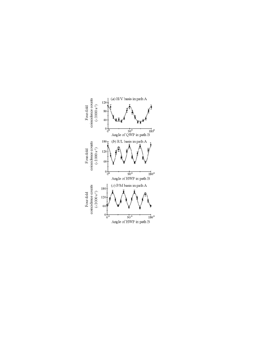
Figure 2: Four–fold coincidence counts for ($a$) fixed $H/V$ polarization measurement basis in path A while rotating QWP in path B, ($b$) fixed $R/L$ basis in path A while rotating HWP in path B, and ($c$) fixed $P/M$ basis in path A while rotating HWP in path B. Note that in Fig. 2($b$), a QWP at 45^∘ was inserted in path B. Maximum and minimum counts were obtained with similar and different polarization settings in each path, respectively. The error bars represent the statistical errors estimated for a Poisson distribution of the measurement results. Pumping power was ($a$) 380 mW, ($b$) 410 mW and ($c$) 420 mW. Solid lines represent the fitted theoretical prediction.

Fig. 2 shows an example of the experimental data. The error bars represent the statistical errors estimated for a Poisson distribution of the measurement results. Fig. 2($a$) shows the results for four–fold coincidence events while rotating the QWP in path B, with the polarization in path A fixed at the $H/V$ basis. The four–fold coincidence counts were maximal at QWP angles of 0^∘, 90^∘ and 180^∘, corresponding to the $H/V$ basis measurement in path B, whereas minimal counts were recorded at 45^∘ and 135^∘ ($R/L$ basis). Taking the averages of these values for $C_{\parallel}$ and $C_{\perp}$ over five experiments, the ratio $r$ was obtained as 0.36 $\pm$ 0.06. As this result satisfies the condition given in Eq. (7), we find that this correlation indicates the successful generation of $ETP$.

Similarly, Fig. 2($b$) (Fig. 2($c$)) shows the results of four–fold coincidence counts with the HWP rotated in path B and $R/L$ ($P/M$) basis measurement setup in path A. In this case, the polarization basis was transformed from the $R/L$ ($H/V$) basis to the $P/M$ ($P/M$) basis, allowing different and similar polarization settings between paths A and B to be measured. Note that in order to transform from the $R/L$ basis to the $P/M$ basis, we set a QWP rotated by 45^∘ before the HWP in path B. The obtained values of the ratio $r$ are 0.38 $\pm$ 0.05 for $R/L$, and 0.36 $\pm$ 0.02 for $P/M$, which also satisfy condition (7) and are consistent with the result in Fig. 2($a$). Figs. 2($a$)–($c$) show a correlation between the same measurement outcomes ($|HV\rangle$, $|RL\rangle$ and $|PM\rangle$), and anti–correlation between different measurement outcomes ($|HV\rangle$–$|RL\rangle$, $|RL\rangle$–$|PM\rangle$ and $|PM\rangle$–$|HV\rangle$). Based on these results, specifically the correlation/anti–correlation ratios $r$ satisfying Eq. (7), it appears that the present system successfully generated $ETP$.

Perfect anti–correlation, which should have been obtained for ideal pure state $ETP$, was not achieved in these experiments. One of the reasons for this may have been the presence of $EOP$ due to a lack of coherence between the two emitted pairs. In the present experimental setup, temporal and spatial coherence was implemented using irises and interference filters. This may not have been sufficient to obtain single mode.

The ratio of $ETP$ among the generated states can be estimated by calculating the four–fold coincidence rates for a mixture of pure state $ETP$ (Eq. (3)) and two independent pure state $EOP$s (Eq. (6)). If we define $\alpha$ as the probability of the generation of pure state $ETP$ given by Eq. (3) and $\beta$ as the probability of generating two independent pure state $EOP$s given by Eq. (6), the four–fold coincidence rates are given by

$$C_{0}\left[\frac{\alpha}{3}\cos^{4}(2\theta_{\lambda/4})+\frac{\beta}{2}\left(\frac{\cos^{4}(2\theta_{\lambda/4})+1}{2}\right)\right],$$ (8)

$$C_{0}\left[\frac{\alpha}{3}\cos^{2}(4\theta_{\lambda/2})+\frac{\beta}{2}\left(\frac{\cos^{2}(4\theta_{\lambda/2})+1}{2}\right)\right],$$ (9)

and

$$C_{0}\left[\frac{\alpha}{3}\sin^{2}(4\theta_{\lambda/2})+\frac{\beta}{2}\left(\frac{\sin^{2}(4\theta_{\lambda/2})+1}{2}\right)\right],$$ (10)

where, Eqs. (8)–(10) correspond to Fig. 2($a$), 2($b$) and 2($c$), respectively. $C_{0}$ is the total rate of four–fold coincidence counts and $\theta_{\lambda/4}$ and $\theta_{\lambda/2}$ are the angle of the QWP and HWP in path B, respectively (solid lines in Figs. 2($a$)–($c$)). Defining $r=C_{\perp}/C_{\parallel}$ as the ratio of the minima and maxima in Eqs. (8)–(10), we obtain the relation between $\alpha$ and $r$ as follows.

$$\alpha=\frac{1-2r}{1-2r/3}.$$ (11)

Therefore, for the ratio of $r$ = 0.36 obtained in our experiments, we obtain an $ETP$ fraction of $\alpha$ = 0.37.

The analysis given above is based on the assumption that the polarization states are the maximally coherent pure states given by Eq. (3) and (6) and that the only source of coincidences between $H/V$ and $R/L$ is the multi-mode component given by the $EOP$ state in Eq. (6). However, decoherence resulting in mixed state outputs may also contribute to such coincidences.

In the present setup, the visibility of the coincidence counts observed for individual $EOP$ emission was about 0.9 at a count rate of 3000 s^-1. In principle, complete quantum tomography would be needed to identify the effects of this decoherence on the two–photon–polarization states. In order to obtain a rough estimate of the effects of decoherence, it may be useful to consider the coincidence counts caused by white noise in the mixed state $EOP$ emission. In this case, the rate of coincidence counts is equal to $1/4$ of the total rate of two pair coincidences, regardless of the polarizations measured. A white noise fraction of $\gamma$ added to the total density matrix therefore adds a constant background coincidence rate of $C_{0}\gamma/4$ to the polarization dependence given by Eqs. (8)–(10).

Since the visibility of 0.9 observed in our experiment suggests a noise background of about 0.1 for one pair, we estimate that the two pair noise may be about $\gamma=0.2$. With this assumption, the single mode component $\alpha$ is raised to 0.46, while the coherent multimode component $\beta$ drops to 0.34. Thus the single mode contribution is increased because the value of $r>0$ observed in the experiment is now partially attributed to the effects of decoherence, reducing the multi–mode contribution necessary to explain the experimentally observed correlations.

A more precise investigation of decoherence effects will be presented elsewhere. Here, it should only be noted that decoherence effects generally increase the ratio $r$, since decoherence reduces the polarization correlations that are responsible for the differences between $C_{\parallel}$ and $C_{\perp}$. The minimal fraction of $ETP$ emission required to explain the observed value of $r<1/2$ is therefore obtained by assuming the emission of pure state $ETP$ and $EOP$, as given in Eqs. (8)–(11). Our method has thus successfully verified the presence of a significant single mode component in the emission footnote2 .

In conclusion, a scheme to distinguish $ETP$ from two independent $EOP$s based on four–fold coincidence has been proposed and demonstrated experimentally. The experimental results indicate the generation of two photons in the same spatiotemporal mode in each path, strongly suggesting the formation of $ETP$. Specifically, we have been able to confirm a minimum of 37$\%$ single mode emission among the entangled four photon states generated in our experimental setup.

We would like to thank J. Hotta, H. Fujiwara, H. Oka, A. G. White and F. Morikoshi for their useful discussions. We also thank D. Kawase, K. Ushizaka and T. Tsujioka for technical support. This work was supported by Core Research for Evolutional Science and Technology, Japan Science and Technology Agency. Part of this work was also supported by the International Communication Foundation.

References

- (1) Z. Y. Ou and L. Mandel, Phys. Rev. Lett. 61, 50 (1988).
- (2) P. G. Kwiat, K. Mattle, H. Weinfurter, A. Zeilinger, A. V. Sergienko and Y. Shih, Phys. Rev. Lett. 75, 4337 (1995).
- (3) P. G. Kwiat, E. Waks, A. G. White, I. Appelbaum, and P. H. Eberhard, Phys. Rev. A 60, R773 (1999).
- (4) D. Bouwmeester, A. Ekert, and A. Zeilinger, The Physics of Quantum Information, 2nd ed. (Springer, Berlin, 2001).
- (5) D. Bouwmeester, J.–W. Pan, M. Daniell, H. Weinfurter, and A. Zeilinger, Phys. Rev. Lett. 82, 1345 (1999).
- (6) J. G. Rarity and P. R. Tapster, Phys. Rev. A 59, R35 (1999).
- (7) J.–W. Pan, D. Bouwmeester, M. Daniell, H. Weinfurter, and A. Zeilinger, Nature (London) 403, 515 (2000).
- (8) M. Eibl, S. Gaertner, M. Bourennane, C. Kurtsiefer, M. Zukowski, and H. Weinfurter, Phys. Rev. Lett. 90, 200403 (2003).
- (9) T. Tsegaye, J. Söderholm, M. Atatüre, A. Trifonov, G. Björk, A. V. Sergienko, B. E. A. Saleh, and M. C. Teich, Phys. Rev. Lett. 85, 5013 (2000).
- (10) J. C. Howell, A. Lamas–Linares, and D. Bouwmeester, Phys. Rev. Lett. 88, 030401 (2002).
- (11) N. Gisin and A. Peres, Phys. Lett. A 162, 15 (1992).
- (12) A. Lamas–Linares, J. C. Howell, and D. Bouwmeester, Nature (London), 412, 887 (2001).
- (13) More precisely, it can be shown that this assumption is generally valid if there is no local polarization, a situation that applies to the present experiment.
- (14) C. Kurtsiefer, M. Oberparleiter, and H. Weinfurter, Phys. Rev. A 64, 023802 (2001).
- (15) It should be noted that the fraction of single mode emission is not related to the amount of entanglement generated, since the fraction is generally mixed state with non–maximal entanglement.