Components for Optical Qubits in the Radio Frequency Basis

Abstract

We describe a scheme for the encoding and manipulation of single photon qubits in radio frequency sideband modes using standard optical elements.

(3 November 2003)

I Introduction

Quantum information can be encoded and manipulated using single photon states. Many in principle demonstrations of quantum information tasks have now been accomplished in single photon optics including quantum cryptography [1], quantum dense coding [2] and quantum teleportation [3]. More recently two qubit gates have been realised [4, 5] using conditional techniques [6]. Such experiments typically make use of polarisation to encode the qubits. However, polarisation is not the only photonic degree of freedom available to the experimentalist. For example schemes in which the timing [7] or occupation [8] of optical modes are the quantum variables have also been realized.

We consider here another possibility: a scheme whereby an optical qubit is encoded in the occupation by a single photon of one of two different frequency modes. Two optical frequency basis states, separated by radio or microwave frequencies, would be sufficiently close together that they could be manipulated with standard electro-optical devices but still clearly resolvable using narrowband optical and opto-electronic systems. There is also the tantalising possibility of implementing such a scheme using commercial optical fibre technologies. Hence, such an encoding scheme is attractive from the perspective of developing stable, robust and ultimately commercially viable optical quantum information systems.

The experimental attraction of developing optical fibre based quantum optical systems is clear. For example, there is ongoing interest in developing non-classical optical sources that will be well suited to optical fibres and optical fibre technologies [9, 10, 11]. Indeed a Quantum Key Distribution (QKD) scheme using radio frequency amplitude and phase modulation as the conjugate bases has recently been demonstrated using optical fibres and fibre technologies [12].

If general experiments in the “radio frequency basis” (RF basis) are to become viable, we would require analogies of the tools of the trade used in polarisation encoding schemes. These tools are principally the half-wave plate (HWP) which is used to make arbitrary rotations of a state in the polarisation basis, the polarising beamsplitter (PBS) which is used to separate (or combine) photons into (from) different spatial and polarisation modes and the quarter-wave plate (QWP) which is used to introduce relative phase shifts between the two bases.

The principle contribution of this work is to introduce and then analyse a device which produces arbitrary rotations in the RF basis - a “Radio Frequency Half-Wave Plate” (RF-HWP). A necessary component of the RF-HWP is a “Frequency Beamsplitter” (FBS) - the RF-basis analogue of the PBS. Previous papers have described a device based on a Fabry-Perot cavity which could be used as a FBS [13, 14]. Here we shall outline a technique that is far less experimentally challenging than that discussed in Ref. [13]. We note that relative phase shifts (that is, QWP action) can be achieved through propagation.

II In Principle

In order to illustrate the physics of the device let us first take an idealized example of an encoding scheme which makes use of the radio frequency basis. Consider the logical basis whereby

$$|{0}\rangle_{L}=|{1}\rangle_{-\Omega}|{0}\rangle_{+\Omega}$$ (1)

$$|{1}\rangle_{L}=|{0}\rangle_{-\Omega}|{1}\rangle_{+\Omega}$$ (2)

where $|{0}\rangle_{L}$ and $|{1}\rangle_{L}$ denote the logical states of the qubit and the notation $|{n}\rangle_{\pm\Omega}$ denotes an $n$ photon state at the frequency $\pm\Omega$ relative to the average or carrier frequency $\omega_{0}$. We shall assume that the states are indistinguishable apart from their frequencies and we note that $\Omega$ is taken to be a radio or microwave frequency in the range of tens of megahertz to a few gigahertz. It is convenient to write the states of Eq.1 in the form

$$|{0}\rangle_{L}=A(-\Omega)^{\dagger}|{0}\rangle$$ (3)

$$|{1}\rangle_{L}=A(+\Omega)^{\dagger}|{0}\rangle$$ (4)

where $A(\omega)^{\dagger}$ is the creation operator for the $\omega$ frequency mode. As all the elements in our device are passive (energy conserving) we can obtain the state evolution produced through the device by considering the Heisenberg evolution of the relevant operators.

Figure 1 illustrates schematically the RF-HWP. We shall assume that all of the beamsplitters are $50\%$ transmitting in our analysis of the system depicted in Fig. 1. We shall additionally make use of the symmetric beamsplitter convention [15]. Let us denote the “forward travelling” beams as those propagating to the right of Fig. 1 and the “backward travelling” beams as those propagating to the left.

In the Heisenberg picture, we define the annihilation operator for the input mode at a particular Fourier frequency $\omega$ relative to the carrier as $A_{in}(\omega)$. We also define an ancilla field ${\hat{v}}_{in}(t)$, initially in a vacuum state, entering the device vertically from the bottom. Fig. 1 defines a number of internal annihilation operators for the RF-HWP as well as two output fields. The output of interest is $A_{out}$.

If we take the logical basis as defined in Eq. 1 and 3, we become interested specifically in the operators, $A_{k}(\Omega)$ and $A_{k}(-\Omega)$ where $k=in,1..6,out,back$. We shall make use of the relation that $A_{k}^{\dagger}(\omega)=A_{k}(-\omega)^{\dagger}$ [16] to find the relevant creation operators.

The first stage of the RF-HWP is essentially a highly asymmetric Mach-Zehnder interferometer. The annihilation operators for the forward travelling outputs of the Mach-Zehnder interferometer at the frequency $\omega$ may be written as

$$A_{1}(\omega) = \frac{1}{2}\left[A_{in}(\omega)\left(-e^{\imath\phi}e^{\imath\omega\tau}+1\right)+\imath v_{in}(\omega)\left(e^{\imath\phi}e^{\imath\omega\tau}+1\right)\right]$$ (5)

$$A_{2}(\omega) = \frac{1}{2}\left[\imath A_{in}(\omega)\left(e^{\imath\phi}e^{\imath\omega\tau}+1\right)+v_{in}(\omega)\left(e^{\imath\phi}e^{\imath\omega\tau}-1\right)\right]$$ (6)

where $A_{1}$ and $A_{2}$ are defined in Fig. 1, $\tau$ is the differential time delay introduced into one of the arms of the interferometer and $\phi=\omega_{0}\tau$ is the phase shift acquired by a field at the carrier frequency

Choosing the time delay $\tau$ in the interferometer such that $\phi=\pi/2$ and $\Omega\tau=\pi/2$, the creation operators for the forward travelling outputs of the Mach-Zehnder interferometer at the frequencies $\omega=\pm\Omega$ are

$$A_{1}(\Omega)^{\dagger} = A_{in}(\Omega)^{\dagger},\quad A_{1}(-\Omega)^{\dagger}=-\imath v_{in}(-\Omega)^{\dagger}$$ (7)

$$A_{2}(\Omega)^{\dagger} = -v_{in}(\Omega)^{\dagger},\quad A_{2}(-\Omega)^{\dagger}=-\imath A_{in}(-\Omega)^{\dagger}$$ (8)

In the state picture we have that an arbitrary input state

$$|{\psi}\rangle=(\mu A_{in}(-\Omega)^{\dagger}+\nu A_{in}(\Omega)^{\dagger})|{0}\rangle_{Ain}|{0}\rangle_{vin}$$ (9)

is transformed to the output state $|{\psi^{\prime}}\rangle$ according to

$$|{\psi^{\prime}}\rangle = U|{\psi}\rangle=U(\mu A_{in}(-\Omega)^{\dagger}+\nu A_{in}(\Omega)^{\dagger})|{0}\rangle_{Ain}|{0}\rangle_{vin}$$ (10)

$$= (\mu UA_{in}(-\Omega)^{\dagger}U^{\dagger}+\nu UA_{in}(\Omega)^{\dagger}U^{\dagger})|{0}\rangle_{A1}|{0}\rangle_{A2}$$ (11)

$$= (\mu\imath A_{2}(-\Omega)^{\dagger}+\nu A_{1}(\Omega)^{\dagger})|{0}\rangle_{A1}|{0}\rangle_{A2}$$ (12)

$$= \imath\mu|{0}\rangle_{A1}|{1}\rangle_{-\Omega,A2}+\nu|{1}\rangle_{+\Omega,A1}|{0}\rangle_{A2}$$ (13)

where $U$ is the unitary operator representing the evolution through the element. In going from lines two to three we have used the fact that $UA_{in}(-\Omega)^{\dagger}U^{\dagger}$ is time reversed Heisenberg evolution, obtained explicitly by inverting the standard Heisenberg equations such that the input operator is written in terms of the output operators. We have also used $U|{0}\rangle_{Ain}|{0}\rangle_{vin}=|{0}\rangle_{A1}|{0}\rangle_{A2}$. We see that the action of an asymmetric Mach-Zehnder on the frequency encoding is equivalent to the action of a polarising beamsplitter in polarisation encoding.

The heart of the RF-HWP is an acousto-optic modulator (AOM). An AOM couples two different frequency and spatial modes together via a phonon interaction [17, 18]. In our scheme the AOM is used to shift photons between the two frequencies $-\Omega$ and $\Omega$. The annihilation operators for the forward travelling outputs of the AOM, $A_{3}(\omega)$ and $A_{4}(\omega)$ as defined in Fig. 1, are [17]

$$A_{3}(\omega) = \cos\theta A_{1}(\omega)+\imath\sin\theta A_{2}(\omega-\delta)$$ (14)

$$A_{4}(\omega) = \cos\theta A_{2}(\omega)+\imath\sin\theta A_{1}(\omega+\delta)$$ (15)

where $\delta$ represents the modulation frequency applied to the AOM and $\theta$ is a measure of the diffraction efficiency of the AOM such that $\cos\theta$ represents the undiffracted fraction of the field and $\sin\theta$ represents the diffracted fraction. We have taken the asymmetric phase convention for the AOM outputs and note that $\theta$ is proportional to the amplitude of the radio frequency modulation applied to the AOM [18]. We note that the second term in Eq. 14 represents the diffracted, and hence frequency upshifted, component of the input field $A_{2}$. Similarly, the second term in Eq. 15 represents the downshifted component of $A_{1}$.

We double pass the AOM in this scheme. The two backward travelling fields $A_{5}$ and $A_{6}$ emerge from the AOM as illustrated in Fig. 1. The annihilation operators for the backward travelling fields emerging from the AOM are

$$A_{5}(\omega) = \cos\theta A_{4}(\omega)+\imath\sin\theta A_{3}(\omega+\delta)$$ (16)

$$= \cos 2\theta A_{2}(\omega)+\imath\sin 2\theta A_{1}(\omega+\delta)$$ (17)

$$A_{6}(\omega) = \cos\theta A_{3}(\omega)+\imath\sin\theta A_{4}(\omega-\delta)$$ (18)

$$= \cos 2\theta A_{1}(\omega)+\imath\sin 2\theta A_{2}(\omega-\delta)$$ (19)

The backward travelling fields $A_{5}$ and $A_{6}$ make a second pass of the Mach-Zehnder interferometer. The annihilation operators for the output fields of the system, $A_{out}$ and $A_{back}$, are

$$A_{out}(\omega) = \frac{1}{2}\left[\imath A_{5}(\omega)\left(e^{\imath\phi}e^{\imath\omega\tau}+1\right)+A_{6}(\omega)\left(e^{\imath\phi}e^{\imath\omega\tau}-1\right)\right]$$ (20)

$$A_{back}(\omega) = \frac{1}{2}\left[A_{5}(\omega)\left(-e^{\imath\phi}e^{\imath\omega\tau}+1\right)+\imath A_{6}(\omega)\left(e^{\imath\phi}e^{\imath\omega\tau}+1\right)\right]$$ (21)

where the parameters $\phi$ and $\tau$ are the same as those for the forward travelling asymmetric Mach-Zehnder interferometer.

We can combine the results of Equations 5, 16, 18, 20 and 21 as well as making use of $A^{\dagger}(\omega)=A(-\omega)^{\dagger}$ to arrive at the creation operators for the outputs of the RF-HWP in terms of the inputs. Focussing on the downward travelling output $A_{out}$ at the frequencies of interest $\omega=\pm\Omega$, setting the AOM modulation frequency $\delta=2\Omega$ and setting $\tau$ such that $\phi=\pi/2$ and $\Omega\tau=\pi/2$, we find that

$$A_{out}(-\Omega)^{\dagger} = -\left[\cos 2\theta A_{in}(-\Omega)^{\dagger}+\sin 2\theta A_{in}(\Omega)^{\dagger}\right]$$ (22)

$$A_{out}(\Omega)^{\dagger} = -\left[\cos 2\theta A_{in}(\Omega)^{\dagger}-\sin 2\theta A_{in}(-\Omega)^{\dagger}\right]$$ (23)

Applying Eq. 22 to the $|{0}\rangle_{L}$ input state leads to

$$|{\psi}\rangle_{0,out} = -\left[\cos 2\theta A_{out}(-\Omega)^{\dagger}-\sin 2\theta A_{out}(\Omega)^{\dagger}\right]|{0}\rangle_{Aout}|{0}\rangle_{vout}$$ (24)

$$= -(\cos 2\theta|{0}\rangle_{L}-\sin 2\theta|{1}\rangle_{L})$$ (25)

whilst applying it to the $|{1}\rangle_{L}$ input gives

$$|{\psi}\rangle_{1,out} = -\left[\cos 2\theta A_{out}(\Omega)^{\dagger}+\sin 2\theta A_{out}(-\Omega)^{\dagger}\right]|{0}\rangle_{Aout}|{0}\rangle_{vout}$$ (26)

$$= -(\cos 2\theta|{1}\rangle_{L}+\sin 2\theta|{0}\rangle_{L})$$ (27)

Equations 24 and 26 are the key results of this paper. Up to a global phase, these equations are formally equivalent to those used to describe the rotation of an arbitrary two dimensional vector through the angle $\Theta=2\theta$. Hence the system illustrated in Fig. 1 is operationally equivalent to a half-wave plate in the basis defined by the frequencies $-\Omega$ and $\Omega$.

III In Practice

The situation considered so far is of course impractical, as single frequency qubits will be stationary in time. More realistically, we might consider finite bandwidth qubits of the form:

$$|{0}\rangle_{L} = ({{2}\over{\pi\sigma}})^{1/4}\int d\omega e^{-(\Omega+\omega)^{2}/\sigma}A_{in}(\omega)^{\dagger}|{0}\rangle$$ (28)

$$|{1}\rangle_{L} = ({{2}\over{\pi\sigma}})^{1/4}\int d\omega e^{-(\Omega-\omega)^{2}/\sigma}A_{in}(\omega)^{\dagger}|{0}\rangle$$ (29)

The overlap between these qubits is

$$\langle 0|1\rangle_{L}=e^{-2\Omega^{2}/\sigma}$$ (30)

thus provided the width of the frequency packet is sufficiently small compared to its mean (i.e $\sigma<<2\Omega^{2}$) then these qubits will be approximately orthogonal. The problem with the finite frequency spread for our device is that now the condition $\Omega\tau=\pi/2$ will not be precisely satified for the entire frequency packet. The effect is to produce a phase shift across the frequency wave packet and also to produce some probability of photons exiting the device in the wrong beam (ie $A_{back}$) or at frequencies outside the computational basis (eg $2\Omega$). Taking such events as lost photons and tracing over them leads to a mixed state which can be written

$$\rho_{out,i}=|{Q}\rangle_{i}\langle{Q}|_{i}+|{\bar{Q}}\rangle\langle{\bar{Q}}|$$ (31)

where $\rho_{out,1}$ represents the mixed state output obtained for the logical state input $|{i}\rangle_{L}$. For the $|{0}\rangle_{L}$ input state

$$|{Q}\rangle_{0} = -({{2}\over{\pi\sigma}})^{1/4}\int d\omega e^{-(\Omega+\omega)^{2}/\sigma}(\cos 2\theta A_{in}(\omega)^{\dagger}1/2(1+e^{i\pi(\Omega+\omega)/\Omega})-$$ (33)

$$\sin 2\theta A_{in}(\omega+2\Omega)^{\dagger}1/4(1+e^{i\pi/2(\Omega+\omega)/\Omega})^{2})|{0}\rangle$$

and for the $|{1}\rangle_{L}$ input

$$|{Q}\rangle_{1} = -({{2}\over{\pi\sigma}})^{1/4}\int d\omega e^{-(\Omega-\omega)^{2}/\sigma}(\cos 2\theta A_{in}(\omega)^{\dagger}1/2(1+e^{-i\pi(\Omega-\omega)/\Omega})+$$ (35)

$$\sin 2\theta A_{in}(\omega-2\Omega)^{\dagger}1/4(1+e^{-i\pi/2(\Omega-\omega)/\Omega})^{2})|{0}\rangle$$

and where $|{\bar{Q}}\rangle$ is a collective ket representing all the photons that end up in (orthogonal) states outside the computational basis. We can evaluate the impact of this effect by calculating the fidelity between the expected output state, $|{P}\rangle_{i}$, and that obtained:

$$F=\langle{P}|\rho_{out,i}|{P}\rangle_{i}$$ (36)

The expression for the fidelity is complicated and of limited utility to reproduce here, however its pertinent features can be listed sucinctly: the fidelity depends strongly on the ratio of $\Omega^{2}$ to $\sigma$; it depends weakly on the rotation angle $\theta$; as expected it tends to one as the ratio $\Omega^{2}/\sigma$ tends to infinity. Some representative results are: $\Omega^{2}/\sigma=10$, $F=0.942$; $\Omega^{2}/\sigma=100$, $F=0.9939$; $\Omega^{2}/\sigma=1000$, $F=0.99938$. We conclude that high fidelities are consistent with sensible signal bandwidths.

Let us now turn to technical issues. Conceptually, the RF-HWP comprises a FBS, followed by an AOM followed by another FBS. However, implementing the RF-HWP in such a fashion would be a tremendously challenging technical task. It would require actively locking the phase $\phi=\pi/2$ in two different interferometers. In addition, the optical path length between the two interferometers would need to be locked. This is why we have proposed the RF-HWP with the folded design illustrated in Fig. 1. This folded design requires locking of only one interferometer. Further, a locking signal can be derived from the backward travelling output of the RF-HWP, $A_{back}$, without disturbing the useful output $A_{out}$.

The technical limitations to the performance of the RF-HWP will be set by the diffraction efficiency of the AOM, the transmission losses of the AOM and the mode-matching efficiency in the interferometer. Rotation of the input through an angle of $\Theta=\pi/2$ requires that the AOM have a diffraction efficiency of $50\%$. This technical requirement can be met with commercially available devices [20]. Transmission losses in the AOM may be modelled as a perfectly transmitting AOM with a partially transmitting beamsplitter placed on each output port. We model mode-matching efficiency in the interferometer similarly. Using this approach, and noting that both the AOM and interferometer are double-passed, we find that the output of the RF-HWP may be written as

$$\rho_{out}^{\prime}=\eta_{T}\rho_{out}+(1-\eta_{T})|{0}\rangle\langle{0}|$$ (37)

where $\rho_{out}^{\prime}$ represents the new output of the RF-HWP after taking account of transmission loss in the AOM ($\eta_{AOM}$) and the mode-matching efficiency of the interferometer ($\eta_{mm}$) [19]. The total transmission of the RF-HWP is $\eta_{T}=\eta_{AOM}^{2}\eta_{mm}^{2}$. We make use of a collective ket $|{0}\rangle$ to represent the vacua introduced within the device. A good quality free-space AOM would have $\eta_{AOM}>0.95$ [20]. Similarly, a well mode-matched interferometer would have $\eta_{mm}>0.95$ [21]. It would therefore be realistic to expect that the RF-HWP could attain total transmission of $\eta_{T}\approx 0.81$ with current commercially available technologies. The effective single-pass transmission of the FBS proposed here would be $\eta_{mm}$.

IV Conclusion

In summary, we have proposed devices which may be used as the principle experimental components in optical quantum imformation systems which make use of the radio frequency basis. These components are essentially the RF basis analogues of the polarising beamsplitter and the half-wave plate. We have shown that an asymmetric Mach-Zehnder interferometer can perform the function of a frequency beamsplitter. We have also shown that this system may be combined with an acousto-optic modulator in a folded design to form a radio frequency half-wave plate. We have shown both devices are feasible using current technologies and could operate with reasonable bandwidths.

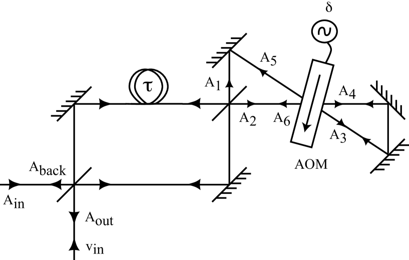
FIG. 1.: A schematic diagram of the proposed system. All of the beamsplitters are $50\%$ transmitting, the internal fields are labelled as $A_{k}$ and the arrows indicate directions of propagation of optical fields. The differential time delay in the two arms of the Mach-Zehnder interferometer is indicated by the time delay $\tau$. The abbreviation AOM stands for acousto-optic modulator and the arrow in the AOM indicates the direction of propagation of the acoustic wave in the device. The frequency of the RF source used to drive the AOM is $\delta$.

- [1] W. T. Buttler et al, Phys. Rev. A57, 2379 (1998).
- [2] K. Mattle, H. Weinfurter, P. G. Kwiat, and A. Zeilinger Phys. Rev. Lett.76, 4656-4659 (1996).
- [3] D. Bouwmeester, J. W. Pan, K. Mattle, M. Eibl, H. Weinfurter and A. Zeilinger, Nature 390, 575 (1997).
- [4] T. B. Pittman, B. C. Jacobs, J. D. Franson, Phys. Rev. Lett., 88, 257902 (2002); T. B. Pittman, M. J. Fitch, B. C. Jacobs and J. D. Franson, quant-ph/0303113 (2003).
- [5] J.L.O’Brien, G.J.Pryde, A.G.White, T.C.Ralph and D.Branning, submitted (2003).
- [6] E. Knill, R. Laflamme, and G. J. Milburn, Nature, 404, 48 (2001).
- [7] H. Zbinden et al, Appl.Phys.B 67, 743 (1998).
- [8] E. Lombardi, F. Sciarrino, S. Popescu, and F. De Martini Phys. Rev. Lett.88, 070402 (2002)
- [9] M. Fiorentino, P. L. Voss, J. E. Sharping, and P. Kumar, IEEE Ph. Technol. Lett., 14, 983 (2002).
- [10] J. E. Sharping, M. Fiorentino, P. Kumar, Opt. Lett., 26, 367 (2001)
- [11] C. Silberhorn, P. K. Lam, O. Weiss, F. Konig, N. Korolkova, G. Leuchs, Phys. Rev. Lett., 86, 4267 (2001).
- [12] J.-M. Merolla, L. Duraffourg, J.-P. Goedgebuer, A. Soujaeff, F. Patois, and W. T. Rhodes, Eur. Phys. J. D, 18, 141 (2002).
- [13] E. H. Huntington and T. C. Ralph J. Opt. B 4, 123 (2002).
- [14] J. Zhang Phys. Rev. A, 67, 054302 (2003)
- [15] D. F. Walls, and G. J. Milburn, Quantum Optics, Springer, Berlin (1995).
- [16] R. J. Glauber, Phys. Rev., 130, 2529 (1963).
- [17] K.J.Resch, S. H. Myrskog, J. S. Lundeen, and A. M. Steinberg, Phys. Rev. A, 64, 056101 (2001).
- [18] E. H. Young, S.-K. Yao, Proc. IEEE, 69, 54 (1981).
- [19] A. I. Lvovsky, H. Hansen, T. Aichele, O. Benson, J. Mlynek and S. Schiller, Phys. Rev. Lett., 87, 050402 (2001).
- [20] See for example http://www.brimrose.com
- [21] B. C. Buchler, P. K. Lam, Hans-A. Bachor, U. L. Andersen, and T. C. Ralph, Phys. Rev. A65, 011803 (2002)